Theoretical and numerical study of lamellar eutectic three-phase growth in ternary alloys

Abstract

We investigate lamellar three-phase patterns that form during the directional solidification of ternary eutectic alloys in thin samples. A distinctive feature of this system is that many different geometric arrangements of the three phases are possible, contrary to the widely studied two-phase patterns in binary eutectics. Here, we first analyze the case of stable lamellar coupled growth of a symmetric model ternary eutectic alloy, using a Jackson-Hunt type calculation in thin film morphology, for arbitrary configurations, and derive expressions for the front undercooling as a function of velocity and spacing. Next, we carry out phase-field simulations to test our analytic predictions and to study the instabilities of the simplest periodic lamellar arrays. For large spacings, we observe different oscillatory modes that are similar to those found previously for binary eutectics and that can be classified using the symmetry elements of the steady-state pattern. For small spacings, we observe a new instability that leads to a change in the sequence of the phases. Its onset can be well predicted by our analytic calculations. Finally, some preliminary phase-field simulations of three-dimensional growth structures are also presented.

I Introduction

Eutectic alloys are of major industrial importance because of their low melting points and their interesting mechanical properties. They are also interesting for physicists because of their ability to form a large variety of complex patterns, which makes eutectic solidification an excellent model system for the study of numerous nonlinear phenomena.

In a binary eutectic alloy, two distinct solid phases co-exist with the liquid at the eutectic point characterized by the eutectic temperature $T_{\rm E}$ and the eutectic concentration $C_{\rm E}$. If the global sample concentration is close to the eutectic concentration, solidification generally results in composite patterns: alternating lamellae of the two solids, or rods of one solid immersed in a matrix of the other, grow simultaneously from the liquid. The fundamental understanding of this pattern-formation process was established by Jackson and Hunt (JH) Jackson and Hunt (1966). They calculated approximate solutions for spatially periodic lamellae and rods that grow at constant velocity $v$, and established that the average front undercooling, that is, the difference between the average front temperature and the eutectic temperature, follows the relation

$$\Delta T=K_{1}v\lambda+\frac{K_{2}}{\lambda},$$ (1)

where $\lambda$ is the width of one lamella pair (or the distance between two rod centers), $v$ is the velocity of the solidification front, and $K_{1}$ and $K_{2}$ are constants whose value depends on the volume fractions of the two solid phases and various materials parameters Jackson and Hunt (1966). The two contributions in Eq. (1) arise from the redistribution of solute by diffusion through the liquid and the curvature of the solid-liquid interfaces, respectively.

The front undercooling is minimal for a characteristic spacing

$$\lambda_{JH}=\sqrt{\frac{K_{2}}{K_{1}v}}.$$ (2)

The spacings found in experiments in massive samples are usually distributed in a narrow range around $\lambda_{JH}$ Trivedi et al. (1991). However, other spacings can be reached in directional solidification experiments by imposing a solidification velocity that varies with time. In this way, the stability of steady-state growth can be probed Ginibre et al. (1997). In agreement with theoretical expections Mannevile (1990), steady-state growth is stable over a range of spacings that is limited by the occurrence of dynamic instabilities. For low spacings, a large-scale lamella (or rod) elimination instability is observed Akamatsu et al. (2004a). For high spacings, the type of instability that can be observed depends on the sample geometry. For thin samples, various oscillatory instabilities and a tilt instability can occur, depending on the alloy phase diagram and the sample concentration. Beyond the onset of these instabilities, stable tilted patterns as well as oscillatory limit cycles can be observed in both experiments and simulations Ginibre et al. (1997); Karma and Sarkissian (1996). For massive samples, a zig-zag instability occurs for lamellar eutectics Akamatsu et al. (2004b); Parisi and Plapp (2008), whereas rods exhibit a shape instability Parisi and Plapp (2010).

In summary, pattern formation in binary eutectics is fairly well understood. However, most materials of practical importance have more than two components. Therefore, eutectic solidification in multicomponent alloys has received increasing attention in recent years. A particularly interesting situation arises in alloy systems that exhibit a ternary eutectic point, at which four phases (three solids and the liquid) coexist. At such a quadruple point, three binary “eutectic valleys”, that is, monovariant lines of three-phase coexistence, meet. The existence of three solid phases implies that there is a far greater variety of possible structures, even in thin samples. Indeed, for two solids $\alpha$ and $\beta$, an array $\alpha\beta\alpha\beta\ldots$ is the only possibility for a composite pattern in a thin sample; the only remaining degree of freedom is the spacing. With an additional $\gamma$ solid, an infinite number of distinct periodic cycles with different sequences of phases are possible. The simplest cycles are $\alpha\beta\gamma\alpha\beta\gamma\ldots$ and $\alpha\beta\alpha\gamma\alpha\beta\alpha\gamma\ldots$ and permutations. Clearly, cycles of arbitrary length, and even non-periodic configurations are possible. An interesting question is then which configurations, if any, will be favored.

In preliminary works, the occurrence of lamellar structures has been reported in experiments in massive samples Kerr et al. (1964); Bao and Durand (1972); Cooksey and Hellawell (1967); Holder and Oliver (1974); Rinaldi et al. (1972); Ruggiero and Rutter (1995); McCartney et al. (1980). The spatio-temporal evolution in ternary eutectic systems was observed in thin samples (quasi-2D experiments) in both metallic Rex et al. (2005) and organic systems Witusiewicz et al. (2006). In both cases, the simultaneous growth of three distinct solid phases from the liquid with a $\left(\alpha\beta\alpha\gamma\right)$, (named ABAC in Ref. Witusiewicz et al. (2006)) stacking was observed. Measurements in both cases revealed that $\lambda^{2}v$ was approximately constant, in agreement with the JH scaling of Eq. (2).

On the theoretical side, models that extend the JH analysis from binary to ternary eutectics for three different growth morphologies (rods and hexagon, lamellar, and semi-regular brick structures) were proposed by Himemiya et al. Himemiya and Umeda (1999). The relation between front undercooling and spacing is still of the form given by Eq. (1), with constants $K_{1}$ and $K_{2}$ that depend on the morphology. The differences between the minimal undercoolings for different morphologies were found to be small. No direct comparison to experiments was given.

Finally, ternary eutectic growth has also been investigated by phase-field methods in Refs. Apel et al. (2004); Hecht et al. (2004), who have studied different stacking sequences formed by $\alpha$ = Ag₂Al, $\beta$ = ($\alpha$ Al) and $\gamma$ = Al₂Cu in the ternary system Al-Cu-Ag, while transients in the ternary eutectic solidification of a transparent In-Bi-Sn alloy were studied both by phase field modeling and experiments Rex et al. (2005).

The purpose of the present paper is to carry out a more systematic investigation of lamellar ternary eutectic growth. The main questions we wish to address are (i) can an extension of the JH theory adequately describe the properties of ternary lamellar arrays and reveal the differences between cycles of different stacking sequences, and (ii) what are the instabilities that can occur in such patterns. To answer these questions, we develop a generalization of the JH theory to ternary eutectics which is capable of describing the front undercoolings of periodic lamellar arrays with arbitrary stacking sequence. Its predictions are systematically compared to phase-field simulations. We use a generic thermodynamically consistent phase-field model Garcke et al. (2004); Nestler et al. (2005). While this model is known to exhibit several thin-interface effects which limit its accuracy Karma and Rappel (1996); Almgren (1998); Kim et al. (1998); Karma (2001); Eschebaria et al. (2004), we show here that we can obtain a very satisfying agreement between theory and simulations if the solid-liquid interfacial free energy is evaluated numerically. In particular, the minimum-undercooling spacings are accurately reproduced for all stacking sequences that we have simulated.

The model is then used to systematically investigate the instabilities of lamellar arrays, in particular for large spacings. We find that, as for binary eutectics, the symmetry elements of the steady-state array determine the possible instability modes. Whereas the calculation of a complete stability diagram is not feasible due to the large number of independent parameters, we find and characterize several new instability modes. Besides these oscillatory modes that are direct analogs of the ones observed in binary eutectics, we also find a new type of instability which occurs at small spacings: cycles in which the same phase appears more than once can undergo an instability during which one of these lamellae is eliminated; the system therefore transits to a different (simpler) cycle. Furthermore, we also find that the occurrence of this type of instability can be well predicted by our generalized JH theory.

The remainder of the paper is organized as follows. In Sec. 2, we develop the generalized JH theory for ternary eutectics and calculate the undercooling-spacing relationships for several simple cycles. In Sec. 3, the phase-field model is outlined and its parameters are related to the ones of the theory. Sec. 4 presents the simulation results concerning both steady-state growth and its instabilities. In Sec. 5, we briefly discuss questions related to pattern selection and present some preliminary simulations in three dimensions. Sec. 6 concludes the paper.

II Theory

We consider a ternary alloy system consisting of components $A,B$ and $C$, which can form three solid phases $\alpha,\beta$, and $\gamma$ upon solidification from the liquid $l$. The concentrations of the components (in molar fractions) are denoted by $c_{A},c_{B}$ and $c_{C}$ and fulfill the constraint

$$c_{A}+c_{B}+c_{C}=1.$$ (3)

This obviously implies that there are only two independent concentration fields.

As is customary, isothermal sections of the ternary phase diagram can be conveniently displayed in the Gibbs simplex. We are interested in alloy systems that exhibit a ternary eutectic point: four-phase coexistence between three solids and the liquid. The isothermal cross-section at the ternary eutectic temperature is displayed in Figure 1, here for the particular example of a completely symmetric phase diagram.

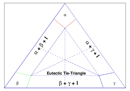
Figure 1: (Color Online) Projection of the ternary phase diagram for a model symmetric ternary eutectic system on the Gibbs simplex. The triangle at the center is the tie-triangle at the eutectic temperature where four phases $\alpha,\beta,\gamma$, and $l$ are in equilibrium. The diagram also contains the information on three-phase equilibria. The liquidus lines corresponding to each of these equilibria (“eutectic valleys”) are shown by dotted lines which meet at the center of the simplex, which is also the concentration of the liquid at which all the three solid phases and the liquid are at equilibrium.

The concentration of the liquid is located in the center of the simplex ($c_{A}=c_{B}=c_{C}=1/3$), and the three solid phases are located at the corners of the eutectic tie triangle. For higher temperatures, no four-phase coexistence is possible, but each pair of solid phases can coexist with the liquid (three-phase coexistence). Each of these three-phase equilibria is a eutectic, and the loci of the liquid concentrations at three-phase coexistence as a function of temperature form three “eutectic valleys” that meet at the ternary eutectic point. On each of the sides of the simplex (with the temperature as additional axis), a binary eutectic phase diagram is found.

The key point for the following analysis is the temperature of solid-liquid interfaces, which depends on the liquid concentration, the interface curvature, and the interface velocity. The dependence on the concentration is described by the liquidus surface, which is a two-dimensional surface over the Gibbs simplex. This surface can hence be characterized by two independent liquidus slopes at each point. For each phase $\nu$ ($\nu=\alpha,\beta,\gamma$), we choose the two liquidus slopes with respect to the minority components. Thus, for the $\alpha$ phase, the interface temperature is given by the generalized Gibbs-Thomson relation,

$$T_{\rm int}^{\alpha}-T_{\rm E}=m_{B}^{\alpha}(c_{B}-c_{B}^{E})+m_{C}^{\alpha}(c_{C}-c_{C}^{E})-\Gamma_{\alpha}\kappa-\frac{v_{n}}{\mu_{\rm int}^{\alpha}},$$ (4)

where $c_{B}$ and $c_{C}$ are the concentrations in the liquid adjacent to the interface, $c_{B}^{E}$ and $c_{C}^{E}$ their values at the ternary eutectic point, and $m^{\alpha}_{B}=\left.\frac{dT_{\alpha}}{dc_{B}}\right|_{c_{C}={\rm const}}$ and $m^{\alpha}_{C}=\left.\frac{dT_{\alpha}}{dc_{C}}\right|_{c_{B}={\rm const}}$ the liquidus slopes taken at the ternary eutectic point. Furthermore, $\Gamma_{\alpha}=\tilde{\gamma}_{\alpha l}T_{\rm E}/L_{\alpha}$ is the Gibbs-Thomson coefficient, with $\tilde{\gamma}_{\alpha l}$ the solid-liquid surface tension and $L_{\alpha}$ the latent heat of fusion per unit volume, and $\mu_{\rm int}^{\alpha}$ is the mobility of the $\alpha$-liquid interface. For the typical (slow) growth velocities that can be attained in directional solidification experiments, the last term, which represents the kinetic undercooling of the interface, is very small. It will therefore be neglected in the following. The expression for the other solid phases are obtained by cyclic permutation of the indices.

In the spirit of the original Jackson-Hunt analysis, for the calculation of the diffusion field in the liquid, the concentration differences between solid and liquid phases are assumed to be constant and equal to their values at the ternary eutectic point. Since we are interested in ternary coupled growth, which will take place at temperatures close to $T_{E}$, this should be a good approximation. Thus, we define

$$\Delta c_{j}^{\nu}=c_{j}^{l}-c_{j}^{\nu}\qquad\mbox{with}\qquad j=A,B,C\qquad\mbox{and}\qquad\nu=\alpha,\beta,\gamma.$$

In this approximation, the Stefan condition at a $\nu$-$l$ interface, which expresses mass conservation upon solidification, reads

$$\partial_{n}c_{j}=-\frac{v_{n}}{D}\Delta c_{j}^{\nu},$$ (5)

where $\partial_{n}c_{j}$ denotes the partial derivative of $c_{j}$ in the direction normal to the interface, $v_{n}$ is the normal velocity of the interface (positive for a growing solid), and $D$ is the chemical diffusion coefficient, for simplicity assumed to be equal for all the components.

We consider a general periodic lamellar array with $M$ repeating units consisting of phases $(\nu_{0},\nu_{1},\nu_{2},\ldots,\nu_{M-1})$ where each $\nu_{i}$ represents the name of one solid phase $\left(\alpha,\beta,\gamma\right)$ in the sequence, with a repeat distance (lamellar spacing) $\lambda$. The width of the $j$-th single solid phase region is $\left(x_{j}-x_{j-1}\right)\lambda$, with $x_{0}=0$ and $x_{M}=1$, and the sum of all the widths corresponding to any given phase is its volume fraction $\eta_{\nu}$. The eutectic front is assumed to grow in the $z$ direction with a constant velocity $v$.

Figure 2: Two examples for periodic lamellar arrays with $M=3$ and $M=4$ units.

II.1 Concentration fields

First, we consider the diffusion fields of the components $A,B,C$ ahead of a growing eutectic front. For the calculation of the concentration fields, the front is supposed to be planar, as in the sketches of Figure 2. We make the following Fourier series expansion for $c_{A}$ and $c_{B}$

$$c_{X}=\sum_{n=-\infty}^{\infty}X_{n}e^{ik_{n}x-q_{n}z}+c_{X}^{\infty},\quad X=A,B.$$ (6)

The third concentration $c_{C}$ follows from the constraint of Eq. (3). In Eq.  (6), $k_{n}=2\pi n/\lambda$ are wave numbers and $q_{n}$ can be determined from the solutions of the stationary diffusion equation

$$v\partial_{z}c_{X}+D\nabla^{2}c_{X}=0,$$

which yields

$$q_{n}=\frac{v}{2D}+\sqrt{k_{n}^{2}+\left(\frac{v}{2D}\right)^{2}}.$$

For all the modes $n\neq 0$, we thus have $q_{n}\simeq|k_{n}|$ for small Peclet number ${\rm Pe}=\lambda/\ell\ll 1$ with $\ell=2D/v_{n}$, which will always be the case for slow growth. The mode $n=0$ describes the concentration boundary layer which is present at off-eutectic concentrations, and which has a characteristic length scale of $\ell$.

To determine the coefficients $X_{n}$ in the above Fourier series, we assume the eutectic front to be at the $z=0$ position. Using the Stefan condition in Eq. (5) and taking the derivative of $c_{X}$ with respect to the $z$-coordinate

$$\partial_{z}c_{X}|_{z=0}=\sum_{n=-\infty}^{\infty}-q_{n}X_{n}e^{ik_{n}x},$$

integration across one lamella period $\lambda$ of arbitrary partitioning of phases gives

$$q_{n}X_{n}\delta_{nm}\lambda = \frac{2}{\ell}\sum_{j=0}^{M-1}\int_{x_{j}\lambda}^{x_{j+1}\lambda}e^{-ik_{m}x}\Delta c_{X}^{\nu_{j}}\>dx,$$ (7)

so that the coefficients $X_{n},n\in{{\rm I}\mkern-3.0mu{\rm N}}$ in the series ansatz, Eq. (6) follow

$$\qquad X_{n} = \frac{4}{\ell q_{n}\lambda k_{n}}\sum_{j=0}^{M-1}\Delta c_{X}^{\nu_{j}}e^{-ik_{n}\lambda(x_{j+1}+x_{j})/2}\sin(k_{n}\lambda(x_{j+1}+x_{j})/2).$$ (8)

Applying symmetry arguments for the sinus and cosinus functions, we can formulate real combinations of these coefficients if we additionally take the negative summation indices into account. We obtain

$$X_{n}+X_{-n}=\frac{8}{\ell q_{n}\lambda k_{n}}\sum_{j=0}^{M-1}\Delta c_{X}^{\nu_{j}}\cos(k_{n}\lambda(x_{j+1}+x_{j})/2)\sin(k_{n}\lambda(x_{j+1}+x_{j})/2),$$

$$i(X_{n}-X_{-n})=\frac{8}{\ell q_{n}\lambda k_{n}}\sum_{j=0}^{M-1}\Delta c_{X}^{\nu_{j}}\sin(k_{n}\lambda(x_{j+1}+x_{j})/2)\sin(k_{n}\lambda(x_{j+1}-x_{j})/2).$$

Herewith, Eq.  (6) reads

$$c_{X}=c_{X}^{\infty}+X_{0}+\sum_{j=0}^{M-1}\sum_{n=1}^{\infty}\frac{8}{\ell q_{n}\lambda k_{n}}\cos(k_{n}\lambda(x_{j+1}+x_{j})/2)\sin(k_{n}\lambda(x_{j+1}+x_{j})/2)\cos(k_{n}x)$$

$$+\sum_{j=0}^{M-1}\sum_{n=1}^{\infty}\frac{8}{\ell q_{n}\lambda k_{n}}\sin(k_{n}\lambda(x_{j+1}+x_{j})/2)\sin(k_{n}\lambda(x_{j+1}-x_{j})/2)\sin(k_{n}x).$$ (9)

The general expression for the mean concentration $\langle c_{X}\rangle_{m}$ ahead of the $m$-th phase of the phase sequence can be calculated to yield

$$\langle c_{X}\rangle_{m} = \frac{1}{(x_{m+1}-x_{m})\lambda}\int_{x_{m}\lambda}^{x_{m+1}\lambda}c_{X}dx$$ (10)

$$= c_{X}^{\infty}+X_{0}+\frac{1}{x_{m+1}-x_{m}}\sum_{n=1}^{\infty}\sum_{j=0}^{M-1}\Big{\{}\frac{16}{\lambda^{2}k_{n}^{2}\ell q_{n}}\Delta c_{X}^{\nu_{j}}\sin[\pi n(x_{m+1}-x_{m})]\times$$

$$\hskip 42.67912pt\times\>\sin[\pi n(x_{j+1}-x_{j})]\cos[\pi n(x_{m+1}+x_{m}-x_{j+1}-x_{j})]\Big{\}}.$$

For a repetitive appearance of a phase $\nu$ in the phase sequence, the mean concentration of component $X$ ahead of this phase follows by taking the weighted average of all the lamellae of phase $\nu$,

$$\langle c_{X}\rangle_{\nu}=\frac{\sum_{m=0}^{M-1}\langle c_{X}\rangle_{m}(x_{m+1}-x_{m})\delta_{{\nu_{m}}\nu}}{\sum_{m=0}^{M-1}(x_{m+1}-x_{m})\delta_{{\nu_{m}}\nu}}\qquad\mbox{with}\qquad\delta_{{\nu_{m}}\nu}=\left\{\begin{array}[]{cc}0&\mbox{for}\>\nu=\nu_{m}\\ 1&\mbox{for}\>\nu\neq\nu_{m}.\end{array}\right.$$ (11)

II.2 Average front temperature

The average front temperature is now found by taking the average of the Gibbs-Thomson equation along the front, separately for each phase ($\alpha,\beta$ and $\gamma$):

$$\Delta T_{\nu} = T_{E}-T_{\nu}=-m_{B}^{\nu}(\langle c_{B}\rangle_{\nu}-c_{B}^{E})-m_{C}^{\nu}(\langle c_{C}\rangle_{\nu}-c_{C}^{E})+\Gamma_{\nu}\langle\kappa\rangle_{\nu},$$ (12)

for $\nu=\alpha,\beta,\gamma$. Here, $\langle\kappa\rangle_{\nu}$ is the average curvature of the solid-liquid interface which can be evaluated by exact geometric relations to be

$$\langle\kappa\rangle_{\nu} = \frac{\sum_{m=0}^{M-1}\langle\kappa\rangle_{m}(x_{m+1}-x_{m})\delta_{{\nu_{m}}\nu}}{\sum_{m=0}^{M-1}(x_{m+1}-x_{m})\delta_{{\nu_{m}}\nu}}$$

and

$$\langle\kappa\rangle_{m}=\frac{\sin\theta_{\nu_{m}\nu_{m+1}}+\sin\theta_{\nu_{m}\nu_{m-1}}}{(x_{m+1}-x_{m})\lambda}.$$

Here, $\theta_{\nu_{m}\nu_{m-1}}$ are the contact angles that are obtained by applying Young’s law at the trijunction points. More precisely, $\theta_{\nu_{m}\nu_{m+1}}$ is the angle, at the triple point (identified by the intersection of the two solid-liquid interfaces and the solid-solid one), between the tangent to the $\nu_{m}-l$ interface and the horizontal (the $x$ direction). For a triple point with the phases $\nu_{m},\nu_{m+1}$ and liquid, the two contact angles $\theta_{\nu_{m}\nu_{m+1}},\theta_{\nu_{m+1}\nu_{m}}$ satisfy the following relations, obtained from Young’s law,

$$\frac{\tilde{\gamma}_{\nu_{m+1}l}}{\cos(\theta_{\nu_{m}\nu_{m+1}})}=\frac{\tilde{\gamma}_{\nu_{m}l}}{\cos(\theta_{\nu_{m+1}\nu_{m}})}=\frac{\tilde{\gamma}_{\nu_{m}\nu_{m+1}}}{\sin(\theta_{\nu_{m}\nu_{m+1}}+\theta_{\nu_{m+1}\nu_{m}})}.$$ (13)

Note that, in general, $\theta_{\nu_{m}\nu_{m+1}}\neq\theta_{\nu_{m+1}\nu_{m}}$.

A short digression is in order to motivate the closure of our system of equations. Although we have not given the explicit expressions, the coefficients $A_{0}$ and $B_{0}$ can be simply calculated by using Eq. (7) with $n=0$. However, to carry out this calculation, the width of each lamella has to be given. If these widths are chosen consistent with the lever rule, that is, the cumulated lamellar width of phase $\nu$ corresponds to the nominal volume fraction of phase $\nu$ for the given sample concentration $c_{A}^{\infty}$, $c_{B}^{\infty}$, and $c_{C}^{\infty}$, the use of Eq. (7) yields $X_{0}=c_{X}^{E}-c_{X}^{\infty}$ ($X=A,B,C$). However, this result is incorrect: the concentrations of the solids are not equal to the equilibrium concentrations at the eutectic temperature because solidification takes place at a temperature below $T_{\bf E}$. Therefore, the true volume fractions depend on the solidification conditions. Their determination would require a self-consistent calculation which is exceedingly difficult. Therefore, we will take the same path as Jackson and Hunt in their original paper Jackson and Hunt (1966): we will assume that the volume fractions of the three phases are fixed by the lever rule at the eutectic temperature, but we will treat the amplitudes of the two boundary layers, $A_{0}$ and $B_{0}$, as unknowns. As in Ref. Jackson and Hunt (1966), one can expect that the difference to the true solution is of order $\rm Pe$ and therefore small for slow solidification.

With this assumption, the equations developed above can now be used in two ways. For isothermal solidification, the temperatures of all interfaces must be equal to the externally set temperature, and the three equations $\Delta T_{\nu}=\Delta T$ for $\nu=\alpha,\beta,\gamma$, can be used to determine the three unknowns $A_{0},B_{0}$ and the velocity $v$ of the solid-liquid front. All of these quantities will be a function of the lamellar spacing $\lambda$. In directional solidification, the growth velocity in steady state is fixed and equal to the speed with which the sample is pulled from a hot to a cold region. The third unknown is now the total front undercooling. In the classic Jackson-Hunt theory for binary eutectics, the system of equations is closed by the hypothesis that the average undercoolings of the two phases are equal. This is only an approximation which is quite accurate for eutectics with comparable volume fractions of the two solids, but becomes increasingly inaccurate when the volume fractions are asymmetric Karma and Sarkissian (1996). We will use the same approximation for the ternary case here, and set $\Delta T_{\alpha}=\Delta T_{\beta}=\Delta T_{\gamma}=\Delta T$. This then leads to expressions for $\Delta T$ as a function of the growth speed $v$ and the lamellar spacing $\lambda$.

II.3 Examples

II.3.1 Binary systems

As a benchmark for both our calculations and simulations, we consider binary eutectic systems with components $A$ and $B$ and with three phases: $\alpha,\beta$, and liquid.

Figure 3: Sketch of a lamellar structure in a binary eutectic system with period length $M=2$. $\nu_{i}$ denotes a phase in the sequence $(\alpha\beta)$.

Setting $x_{0}=0,x_{1}=\eta_{\alpha}$, $x_{2}=1$, and applying Eq. (10) gives

$$\langle c_{X}\rangle_{\alpha} = c_{X}^{\infty}+X_{0}+\frac{1}{\eta_{\alpha}}\sum_{n=1}^{\infty}\Big{\{}\frac{16}{\lambda^{2}k_{n}^{2}\ell q_{n}}\left(\Delta c_{X}^{\alpha}-\Delta c_{X}^{\beta}\right)\sin^{2}(\pi n\eta_{\alpha})\Big{\}}$$ (14)

$$\cong c_{X}^{\infty}+X_{0}+\frac{2\lambda}{\eta_{\alpha}\ell}{\cal P}(\eta_{\alpha})\Delta c_{X}\qquad\mbox{and}$$ (15)

$$\langle c_{X}\rangle_{\beta} = c_{X}^{\infty}+X_{0}-\frac{2\lambda}{(1-\eta_{\alpha})\ell}{\cal P}(1-\eta_{\alpha})\Delta c_{X}$$ (16)

with $k_{n}=2\pi n/\lambda,q_{n}\approx k_{n},\lambda/\ell\ll 1,\Delta c_{X}=\Delta c_{X}^{\alpha}-\Delta c_{X}^{\beta}$, and the dimensionless function

$${\cal P}(\eta) = \sum_{n=1}^{\infty}\frac{1}{(\pi n)^{3}}\sin^{2}(\pi n\eta)$$ (17)

which has the properties ${\cal P}(\eta)={\cal P}(1-\eta)={\cal P}(\eta-1)$.

Furthermore, Eq. (12) together with $\ell=2D/v$ leads to

$$\Delta T_{\alpha}=-m_{B}^{\alpha}B_{0}-\frac{\lambda v}{\eta_{\alpha}D}{\cal P}(\eta_{\alpha})m_{B}^{\alpha}\Delta c_{B}+\Gamma_{\alpha}\langle\kappa\rangle_{\alpha},$$ (18)

$$\Delta T_{\beta}=-m_{A}^{\beta}A_{0}-\frac{\lambda v}{\eta_{\beta}D}{\cal P}(\eta_{\beta})m_{A}^{\beta}\Delta c_{A}+\Gamma_{\beta}\langle\kappa\rangle_{\beta},$$ (19)

where $\langle\kappa\rangle_{\alpha}=2\sin\theta_{\alpha\beta}/(\eta_{\alpha}\lambda)$ and $\langle\kappa\rangle_{\beta}=2\sin\theta_{\beta\alpha}/(\eta_{\beta}\lambda)$. In addition, for a binary alloy $B_{0}=-A_{0}$. The unknown $A_{0}$ and the global front undercooling are determined using the assumption of equal interface undercoolings, $\Delta T_{\alpha}=\Delta T_{\beta}$. The result is identical to the one of the Jackson-Hunt analysis.

II.3.2 Ternary Systems

Next, we study ternary systems with three components ($A,B,C$) and four phases ($\alpha,\beta,\gamma$ and liquid). We start with the configuration $\left(\alpha\beta\gamma\alpha\beta\gamma\ldots\right)$, sketched in Figure 4.

Figure 4: Sketch of a ternary stacking order $\left(\alpha\beta\gamma\right)$ with period length $M=3$.

We set $x_{0}=0,x_{1}=\eta_{\alpha},x_{2}=\eta_{\alpha}+\eta_{\beta}=1-\eta_{\gamma}$ and $x_{3}=1$ and apply Eq. (10). This yields

$$\langle c_{X}\rangle_{\alpha} = c_{X}^{\infty}+X_{0}+\frac{2\lambda}{\eta_{\alpha}\ell}\Big{(}{\cal P}(\eta_{\alpha})\Delta c_{X}^{\alpha}+{\cal Q}(\eta_{\alpha},\eta_{\beta})\Delta c_{X}^{\beta}+{\cal Q}(\eta_{\alpha},\eta_{\gamma})\Delta c_{X}^{\gamma}\Big{)}$$ (20)

$$\langle c_{X}\rangle_{\beta} = c_{X}^{\infty}+X_{0}+\frac{2\lambda}{\eta_{\beta}\ell}\Big{(}{\cal Q}(\eta_{\beta},\eta_{\alpha})\Delta c_{X}^{\alpha}+{\cal P}(\eta_{\beta})\Delta c_{X}^{\beta}+{\cal Q}(\eta_{\beta},\eta_{\gamma})\Delta c_{X}^{\gamma}\Big{)}$$ (21)

$$\langle c_{X}\rangle_{\gamma} = c_{X}^{\infty}+X_{0}+\frac{2\lambda}{\eta_{\gamma}\ell}\Big{(}{\cal Q}(\eta_{\gamma},\eta_{\alpha})\Delta c_{X}^{\alpha}+{\cal Q}(\eta_{\gamma},\eta_{\beta})\Delta c_{X}^{\beta}+{\cal P}(\eta_{\gamma})\Delta c_{X}^{\gamma}\Big{)}.$$ (22)

Here, we have used $X=A,B,C$ and ${\cal P}$ is the function defined in Eq. (17), and

$${\cal Q}(\eta_{\nu_{i}},\eta_{\nu_{j}}) = \sum_{n=1}^{\infty}\frac{1}{(\pi n)^{3}}\sin(\pi n\eta_{\nu_{i}})\sin(\pi n\eta_{\nu_{j}})\cos[\pi n(\eta_{\nu_{i}}+\eta_{\nu_{j}})]$$ (23)

${\cal P}(\eta_{\nu_{i}})$ and ${\cal Q}(\eta_{\nu_{i}},\eta_{\nu_{j}})$ fulfill the properties ${\cal P}(\eta_{\nu_{i}})=-{\cal Q}(\eta_{\nu_{i}},-\eta_{\nu_{i}})$ and ${\cal Q}(\eta_{\nu_{i}},\eta_{\nu_{j}})={\cal Q}(\eta_{\nu_{j}},\eta_{\nu_{i}})$.

For simplicity, we now consider a completely symmetric ternary eutectic configuration: a completely symmetric ternary phase diagram (that is, any two phases can be exchanged without changing the phase diagram) and equal phase fractions $\eta_{\alpha}=\eta_{\beta}=\eta_{\gamma}=\frac{1}{3}$, which implies $c_{X}^{\infty}=c_{X}^{E}$. As a consequence, $X_{0}=0$, and Eq. (20) simplifies to

$$\langle c_{A}\rangle_{\alpha}-c_{A}^{E} = \frac{2\lambda}{\eta_{\alpha}\ell}{\cal P}(\eta_{\alpha})(\Delta c_{A}^{\alpha}-\Delta c_{A}^{\beta})$$ (24)

$$\langle c_{B}\rangle_{\alpha}-c_{B}^{E} = \frac{\lambda{\cal P}(\eta_{\alpha})}{\eta_{\alpha}\ell}\Big{(}\Delta c_{B}^{\alpha}-\Delta c_{B}^{\beta}\Big{)}$$ (25)

$$\langle c_{C}\rangle_{\alpha}-c_{C}^{E} = \frac{\lambda{\cal P}(\eta_{\alpha})}{\eta_{\alpha}\ell}\Big{(}\Delta c_{C}^{\alpha}-\Delta c_{C}^{\gamma}\Big{)},$$ (26)

for the three components. Since, in this case, all phases have the same undercooling by symmetry, the front undercooling is simply given by

$$\Delta T=-\frac{2\lambda v}{\eta_{\alpha}D}{\cal P}(\eta_{\alpha})m_{B}^{\alpha}\Delta c_{B}+\Gamma_{\alpha}\langle\kappa\rangle_{\alpha}$$ (27)

where $\langle\kappa\rangle_{\alpha}=\tfrac{2}{\eta_{\alpha}\lambda}(\sin\theta_{\alpha\beta}+\sin\theta_{\alpha\gamma})$. The terms $\Delta c_{B}^{\alpha}-\Delta c_{B}^{\beta}$ and $\Delta c_{C}^{\alpha}-\Delta c_{C}^{\gamma}$ are identical. For convenience, we write the preceding equation using the term we already use for the binaries namely $\Delta c_{B}=\Delta c_{B}^{\alpha}-\Delta c_{B}^{\beta}$.

Next, we discuss again a ternary eutectic alloy with three components and four phases, but now for the phase cycle $\left(\alpha\beta\alpha\gamma\alpha\beta\ldots\right)$.

Figure 5: Schematic drawing of a ternary eutectic system with a configuration $\left(\alpha\beta\alpha\gamma\alpha\beta\ldots\right)$ of periodic length $M=4$.

Furthermore, we suppose that the two lamellae of the $\alpha$ phase have equal width $\lambda\eta_{\alpha}/2$. The average concentrations $\langle c_{X}\rangle_{m}$ are deduced from the general expression in Eq.10 and read

$$\langle c_{X}\rangle_{\alpha} = c_{X}^{\infty}+X_{0}+\frac{2\lambda}{\tfrac{\eta_{\alpha}}{2}\ell}\Big{(}{\cal S}(\eta_{\alpha},\eta_{\beta})\Delta c_{X}^{\alpha}+{\cal Q}(\tfrac{\eta_{\alpha}}{2},\eta_{\beta})\Delta c_{X}^{\beta}+{\cal Q}(\tfrac{\eta_{\alpha}}{2},\eta_{\gamma})\Delta c_{X}^{\gamma}\Big{)}$$ (28)

$$\langle c_{X}\rangle_{\beta} = c_{X}^{\infty}+X_{0}+\frac{2\lambda}{\eta_{\beta}\ell}\Big{(}2{\cal Q}(\eta_{\beta},\tfrac{\eta_{\alpha}}{2})\Delta c_{X}^{\alpha}+{\cal P}(\eta_{\beta})\Delta c_{X}^{\beta}+{\cal R}(\eta_{\beta},\eta_{\gamma})\Delta c_{X}^{\gamma}\Big{)}$$ (29)

$$\langle c_{X}\rangle_{\gamma} = c_{X}^{\infty}+X_{0}+\frac{2\lambda}{\eta_{\gamma}\ell}\Big{(}2{\cal Q}(\eta_{\gamma},\tfrac{\eta_{\alpha}}{2})\Delta c_{X}^{\alpha}+{\cal R}(\eta_{\gamma},\eta_{\beta})\Delta c_{X}^{\beta}+{\cal P}(\eta_{\gamma})\Delta c_{X}^{\gamma}\Big{)},$$ (30)

where $X=A,B,C$. Furthermore, we have introduced the short notations

$${\cal R}(\eta_{\nu_{i}},\eta_{\nu_{j}}) = \sum_{n=1}^{\infty}\frac{1}{(\pi n)^{3}}\sin(\pi n\eta_{\nu_{i}})\sin(\pi n\eta_{\nu_{j}})\cos(\pi n)$$ (31)

$${\cal S}(\eta_{\nu_{i}},\eta_{\nu_{j}}) = \sum_{n=1}^{\infty}\frac{1}{(\pi n)^{3}}\sin^{2}(\pi n\eta_{\nu_{i}}/2)\{1+\cos(\pi n)\cos[\pi n(\eta_{\nu_{j}}-\eta_{\nu_{i}})]\}.$$ (32)

From the general formulation of the Gibbs-Thomson equation in Eq. (12), we determine the undercoolings,

$$\Delta T_{\alpha} = -m_{B}^{\alpha}\left(B_{0}+\frac{4\lambda}{\eta_{\alpha}\ell}\Big{(}{\cal S}(\eta_{\alpha},\eta_{\beta})\Delta c_{B}^{\alpha}+{\cal Q}(\tfrac{\eta_{\alpha}}{2},\eta_{\beta})\Delta c_{B}^{\beta}+{\cal Q}(\tfrac{\eta_{\alpha}}{2},\eta_{\gamma})\Delta c_{B}^{\gamma}\Big{)}\right)$$ (33)

$$+ -m_{C}^{\alpha}\left(C_{0}+\frac{4\lambda}{\eta_{\alpha}\ell}\Big{(}{\cal S}(\eta_{\alpha},\eta_{\beta})\Delta c_{C}^{\alpha}+{\cal Q}(\tfrac{\eta_{\alpha}}{2},\eta_{\beta})\Delta c_{C}^{\beta}+{\cal Q}(\tfrac{\eta_{\alpha}}{2},\eta_{\gamma})\Delta c_{C}^{\gamma}\Big{)}\right)$$

$$+ \Gamma_{\alpha}\dfrac{2\left(\sin\theta_{\alpha\beta}+\sin\theta_{\alpha\gamma}\right)}{\eta_{\alpha}\lambda}$$

$$\Delta T_{\beta} = -m_{A}^{\beta}\left(A_{0}+\frac{2\lambda}{\eta_{\beta}\ell}\Big{(}2{\cal Q}(\eta_{\beta},\tfrac{\eta_{\alpha}}{2})\Delta c_{A}^{\alpha}+{\cal P}(\eta_{\beta})\Delta c_{A}^{\beta}+{\cal R}(\eta_{\beta},\eta_{\gamma})\Delta c_{A}^{\gamma}\Big{)}\right)$$ (34)

$$+ -m_{C}^{\beta}\left(C_{0}+\frac{2\lambda}{\eta_{\beta}\ell}\Big{(}2{\cal Q}(\eta_{\beta},\tfrac{\eta_{\alpha}}{2})\Delta c_{C}^{\alpha}+{\cal P}(\eta_{\beta})\Delta c_{C}^{\beta}+{\cal R}(\eta_{\beta},\eta_{\gamma})\Delta c_{C}^{\gamma}\Big{)}\right)$$

$$+ \Gamma_{\beta}\dfrac{2\sin\theta_{\beta\alpha}}{\eta_{\beta}\lambda}$$

$$\Delta T_{\gamma} = -m_{A}^{\gamma}\left(A_{0}+\frac{2\lambda}{\eta_{\gamma}\ell}\Big{(}2{\cal Q}(\eta_{\gamma},\tfrac{\eta_{\alpha}}{2})\Delta c_{A}^{\alpha}+{\cal R}(\eta_{\gamma},\eta_{\beta})\Delta c_{A}^{\beta}+{\cal P}(\eta_{\gamma})\Delta c_{A}^{\gamma}\Big{)}\right)$$ (35)

$$+ -m_{B}^{\gamma}\left(B_{0}+\frac{2\lambda}{\eta_{\gamma}\ell}\Big{(}2{\cal Q}(\eta_{\gamma},\tfrac{\eta_{\alpha}}{2})\Delta c_{B}^{\alpha}+{\cal R}(\eta_{\gamma},\eta_{\beta})\Delta c_{B}^{\beta}+{\cal P}(\eta_{\gamma})\Delta c_{B}^{\gamma}\Big{)}\right)$$

$$+ \Gamma_{\gamma}\dfrac{2\sin\theta_{\gamma\alpha}}{\eta_{\gamma}\lambda}.$$

For a symmetric phase diagram (all slopes equal, $m_{X}^{\nu_{i}}=m$) one can show using the assumption of equal undercooling of all phases that an expression for the global interface undercooling can be derived as $\Delta T=1/3(\Delta T_{\alpha}+\Delta T_{\beta}+\Delta T_{\gamma})$ by elimination of the constants $A_{0},B_{0}$ and $C_{0}$ using the relation $(A_{0}+B_{0}+C_{0})=0$.

II.4 Discussion

A point which merits closer attention is the question which of all the possible steady-state configurations exhibits the lowest undercooling. Whereas the general idea that a eutectic system will always select the state of lowest undercooling is wrong (see Sec. V below), an information about this point constitutes nevertheless a useful starting point. Whereas the general solution to this problem is non-trivial, in the following we present some partial insights.

Let us, for the sake of discussion, first compute the average total curvature undercooling $\Delta T_{\kappa}$ of an arbitrary arrangement. Consider a configuration of period M having $M_{a}$ lamella of the $\alpha$ phase, $M_{b}$ lamella of the $\beta$ phase, and $M_{c}$ lamella of the $\gamma$ phase, where the integers $M_{a}$, $M_{b}$, and $M_{c}$ add up to M. In a system where all the solid-liquid and solid-solid surface tensions are identical, the total average curvature undercooling $\Delta T_{\kappa}^{\nu}$ of each phase $\nu$ is,

$$\Delta T_{\kappa}^{\alpha} = \Gamma_{\alpha}\dfrac{2\sin\theta}{\lambda}\dfrac{M_{a}}{\eta_{\alpha}}$$ (36)

$$\Delta T_{\kappa}^{\beta} = \Gamma_{\beta}\dfrac{2\sin\theta}{\lambda}\dfrac{M_{b}}{\eta_{\beta}}$$ (37)

$$\Delta T_{\kappa}^{\gamma} = \Gamma_{\gamma}\dfrac{2\sin\theta}{\lambda}\dfrac{M_{c}}{\eta_{\gamma}}.$$ (38)

It is remarkable that the average curvature undercooling is independent of the individual widths of each lamella, but depends only on the total volume fraction and the number of lamellae of the specific phase. Furthermore, it is quite clear from the above examples that the final expression for the global average interface undercooling can always be written in the same form as Eq. (1). The second term of this expression (that is, the one proportional to $1/\lambda$) can be computed for the case where all Gibbs-Thomson coefficients and liquidus slopes are equal, and reads

$$\dfrac{K_{2}}{\lambda} = \dfrac{\Delta T_{\kappa}^{\alpha}+\Delta T_{\kappa}^{\beta}+\Delta T_{\kappa}^{\gamma}}{3}$$ (39)

$$= \Gamma\dfrac{2\sin\theta}{3\lambda}\left(\dfrac{M_{a}}{\eta_{\alpha}}+\dfrac{M_{b}}{\eta_{\beta}}+\dfrac{M_{c}}{\eta_{\gamma}}\right).$$

For the special case of a completely symmetric phase diagram and a sample at the eutectic composition, Eqn.(39) yields

$$\dfrac{K_{2}}{\lambda} = \Gamma\dfrac{2\sin\theta}{\lambda}\left(M_{a}+M_{b}+M_{c}\right),$$ (40)

where we have used the fact that $\eta_{\alpha}=\eta_{\beta}=\eta_{\gamma}=1/3$. Using, $M_{a}+M_{b}+M_{c}=M$, $\dfrac{K_{2}}{\lambda}=\Gamma\dfrac{2\sin\theta}{\left(\lambda\right/M)}$. Thus, we see that the magnitude of this term per unit lamella in an arrangement is the same for all the possible arrangements, irrespective of the individual widths of the lamella and the relative positions of the lamellae in a configuration. Moreover, we see that for a general off-eutectic composition, choosing the number of lamellae in the ratio $\eta_{\alpha}:\eta_{\beta}:\eta_{\gamma}$ renders the average curvature undercoolings of all the three phases equal. This condition is, however, relevant only for the special case of identical solid-solid and solid-liquid surface tensions and equal liquidus slopes of the phases. For the case when the solid-liquid and solid-solid surface tensions are unequal, the curvature undercooling is no longer independent of the arrangement of the lamella in the configuration. Hence, the problem of determining the minimum undercooling configuration is complex and no general expression regarding the number, position and widths of lamellae can be derived.

Another point is worth mentioning. Under the assumption that the volume fractions of the solid phases are fixed by the lever rule, the width of the three lamellae in the $\alpha\beta\gamma$ cycle is uniquely fixed by the alloy concentration. However, for the $\alpha\beta\alpha\gamma$ cycle, and more generally for any cycle with $M>3$, this is not the case any more because there have to be at least two lamellae of the same phase in the cycle. Whereas the cumulated width of these lamellae is fixed by the global concentration, the width of each individual lamella is not. For example, in the $\alpha\beta\alpha\gamma$ cycle at the eutectic concentration $c_{A}^{\infty}=c_{B}^{\infty}=c_{C}^{\infty}=1/3$, all the configurations $(\xi,1/3,1/3-\xi,1/3)$ for $0<\xi<1/3$ are admissible, where the notation $(\cdot,\cdot,\ldots)$ is a shorthand for the list of the lamella widths $x_{n+1}-x_{n}$. The number $\xi$ is an internal degree of freedom that can be freely chosen by the system. With our method, the global front undercooling can be calculated for any value of $\xi$. For the $\alpha\beta\alpha\gamma$ cycle, we found that the configuration with equal widths of the $\alpha$ phases ($\xi=1/6$) was the one with the minimum average front undercooling. This gives a strong indication that this value is stable, and that perturbations of $\xi$ around this value should decay with time. Hence, the analytic expressions given above for the $\alpha\beta\alpha\gamma$ cycle, which are for $\xi=1/6$, should be the relevant ones.

III Phase-field Model

III.1 Model

A thermodynamically consistent phase-field model is used for the present study Garcke et al. (2004); Nestler et al. (2005). The equations are derived from an entropy functional of the form

$${\cal S}\left(e,\mbox{\boldmath{$c$}},\mbox{\boldmath{$\phi$}}\right) = \int_{\Omega}\left(s\left(e,\mbox{\boldmath{$c$}},\mbox{\boldmath{$\phi$}}\right)-\left(\epsilon a\left(\mbox{\boldmath{$\phi$}},\nabla\mbox{\boldmath{$\phi$}}\right)+\dfrac{1}{\epsilon}w\left(\mbox{\boldmath{$\phi$}}\right)\right)\right)d\Omega,$$ (41)

where $e$ is the internal energy density, $c$ = $(c_{i})_{i=1}^{K}$ is a vector of concentration variables, $K$ being the number of components, and $\mbox{\boldmath{$\phi$}}=\left(\phi_{\alpha}\right)_{\alpha=1}^{N}$ is a vector of phase-field variables, $N$ being the number of phases present in the system. $\phi$ and $c$ fulfill the constraints

$$\sum_{i=1}^{K}c_{i}=1\qquad\mbox{and}\qquad\sum_{\alpha=1}^{N}\phi_{\alpha}=1,$$ (42)

so that these vectors always lie in $K-1$- and $N-1$-dimensional planes, respectively. Moreover, $\epsilon$ is the small length scale parameter related to the interface width, $s\left(e,\mbox{\boldmath{$c$}},\mbox{\boldmath{$\phi$}}\right)$ is the bulk entropy density, $a\left(\mbox{\boldmath{$\phi$}},\nabla\mbox{\boldmath{$\phi$}}\right)$ is the gradient entropy density and $w\left(\mbox{\boldmath{$\phi$}}\right)$ describes the surface entropy potential of the system for pure capillary-force-driven problems.

We use a multi-obstacle potential for $w\left(\mbox{\boldmath{$\phi$}}\right)$ of the form

$$w\left(\mbox{\boldmath{$\phi$}}\right)=\left\{\begin{array}[]{ll}\dfrac{16}{\pi^{2}}\displaystyle\sum_{\begin{subarray}{c}\alpha,\beta=1\\ (\alpha<\beta)\end{subarray}}^{N,N}\sigma_{\alpha\beta}\phi_{\alpha}\phi_{\beta}+\displaystyle\sum_{\begin{subarray}{c}\alpha,\beta,\gamma=1\\ (\alpha<\beta<\gamma)\end{subarray}}^{N,N,N}\sigma_{\alpha\beta\gamma}\phi_{\alpha}\phi_{\beta}\phi_{\gamma},&\textrm{if}\hskip 2.84544pt\mbox{\boldmath{$\phi$}}\in\sum\\ \infty,&\textrm{elsewhere}\\ \end{array}\right.$$ (45)

where $\sum=\{\mbox{\boldmath{$\phi$}}\,|\sum_{\alpha=1}^{N}\phi_{\alpha}=1$ and $\phi_{\alpha}\geq 0\}$, $\sigma_{\alpha\beta}$ is the surface entropy density and $\sigma_{\alpha\beta\gamma}$ is a term added to reduce the presence of unwanted third or higher order phase at a binary interface (see below for details).

The gradient entropy density $a\left(\mbox{\boldmath{$\phi$}},\nabla\mbox{\boldmath{$\phi$}}\right)$ can be written as

$$a\left(\mbox{\boldmath{$\phi$}},\nabla\mbox{\boldmath{$\phi$}}\right)=\begin{array}[]{ll}\displaystyle\sum_{\begin{subarray}{c}\alpha,\beta=1\\ (\alpha<\beta)\end{subarray}}^{N,N}\sigma_{\alpha\beta}\left[a_{c}\left(q_{\alpha\beta}\right)\right]^{2}\lvert q_{\alpha\beta}\lvert^{2},\end{array}$$ (47)

where $q_{\alpha\beta}=\left(\phi_{\alpha}\nabla\phi_{\beta}-\phi_{\beta}\nabla\phi_{\alpha}\right)$ is a vector normal to the $\alpha\beta$ interface. The function $a_{c}\left(q_{\alpha\beta}\right)$ describes the form of the anisotropy of the evolving phase boundary. For the present study, we assume isotropic interfaces, and hence $a_{c}\left(q_{\alpha\beta}\right)=1$. Evolution equations for $c$ and $\phi$ are derived from the entropy functional through conservation laws and phenomenological maximization of entropy, respectively Garcke et al. (2004); Nestler et al. (2005). A linearized temperature field with positive gradient $G$ in the growth direction ($z$ axis) is imposed and moved forward with a velocity $v$,

$$T=T_{0}+G(z-vt)$$ (48)

where $T_{0}$ is the temperature at $z=0$ at time $t=0$. The evolution equations for the phase-field variables read

$$\omega\epsilon\partial_{t}\phi_{\alpha}=\epsilon\left(\nabla\cdot a,_{\nabla\phi_{\alpha}}\left(\mbox{\boldmath{$\phi$}},\nabla\mbox{\boldmath{$\phi$}}\right)-a,_{\phi_{\alpha}}\left(\mbox{\boldmath{$\phi$}},\nabla\mbox{\boldmath{$\phi$}}\right)\right)-\dfrac{1}{\epsilon}w,_{\phi_{\alpha}}\left(\mbox{\boldmath{$\phi$}}\right)-\dfrac{f,_{\phi_{\alpha}}(\mbox{\boldmath{$c$}},\mbox{\boldmath{$\phi$}};T)}{T}-\Lambda,$$ (49)

where $\Lambda$ is the Lagrange multiplier which maintains the constraint of Eq. (42) for $\phi$, and the constant $\omega$ is the relaxation time of the phase fields. Furthermore, $a,_{\nabla\phi_{\alpha}}$, $a,_{\phi_{\alpha}}$, $w,_{\phi_{\alpha}}$ and $f,_{\phi_{\alpha}}$ indicate the derivatives of the respective entropy densities with respect to $\nabla\phi_{\alpha}$ and $\phi_{\alpha}$. The function $f(\mbox{\boldmath{$c$}},\mbox{\boldmath{$\phi$}};T)$ in Eq. (49) describes the free energy density, and is related to the entropy density $s(\mbox{\boldmath{$c$}},\mbox{\boldmath{$\phi$}};T)$, through the relation $f(\mbox{\boldmath{$c$}},\phi;T)=e(\mbox{\boldmath{$c$}},\phi;T)-Ts(\mbox{\boldmath{$c$}},\mbox{\boldmath{$\phi$}};T)$, where $e(\mbox{\boldmath{$c$}},\phi;T)$ is the internal energy density. The free energy density is given by the summation over all bulk free energy contributions $f_{\alpha}(\mbox{\boldmath{$c$}};T)$ of the individual phases in the system. We use an ideal solution model,

$$f(\mbox{\boldmath{$c$}},\mbox{\boldmath{$\phi$}};T)=\sum_{i=1}^{K}\left(Tc_{i}\ln c_{i}+\sum_{\alpha=1}^{N}c_{i}L_{i}^{\alpha}\dfrac{\left(T-T_{i}^{\alpha}\right)}{T_{i}^{\alpha}}h_{\alpha}\left(\mbox{\boldmath{$\phi$}}\right)\right),$$ (50)

where

$$f_{\alpha}(\mbox{\boldmath{$c$}};T)=\sum_{i=1}^{K}\left(Tc_{i}\ln c_{i}+c_{i}L_{i}^{\alpha}\dfrac{\left(T-T_{i}^{\alpha}\right)}{T_{i}^{\alpha}}\right)$$ (51)

is the free energy density of the $\alpha$ solid phase, and

$$f_{l}(\mbox{\boldmath{$c$}};T)=T\sum_{i=1}^{K}\left(c_{i}\ln\left(c_{i}\right)\right)$$ (52)

is the one of the liquid. The parameters $L_{i}^{\alpha}$ and $T_{i}^{\alpha}$ denote the latent heats and the melting temperatures of the $i^{th}$ component in the $\alpha$ phase, respectively. We choose the liquid as the reference state, and hence $L_{i}^{l}=0$.

The function $h_{\alpha}(\mbox{\boldmath{$\phi$}})$ is a weight function which we choose to be of the form $h_{\alpha}\left(\mbox{\boldmath{$\phi$}}\right)=\phi_{\alpha}^{2}\left(3-2\phi_{\alpha}\right)$. Thus, $f=f_{\alpha}$ for $\phi_{\alpha}=1$. Other interpolation functions involving other components of the $\phi$ vector could also be used, but here we restrict ourselves to this simple choice.

The evolution equations for the concentration fields are derived from Eq. (41),

$$\partial_{t}c_{i}=-\nabla\cdot\left(M_{i0}(\mbox{\boldmath{$c$}},\mbox{\boldmath{$\phi$}})\nabla\dfrac{1}{T}+\sum_{j=1}^{K}M_{ij}\left(\mbox{\boldmath{$c$}},\mbox{\boldmath{$\phi$}}\right)\nabla\left(\dfrac{1}{T}\dfrac{\partial f(\mbox{\boldmath{$c$}},\mbox{\boldmath{$\phi$}};T)}{\partial c_{j}}\right)\right).$$ (53)

By a convenient choice of the mobilities $M_{ij}\left(\mbox{\boldmath{$c$}},\mbox{\boldmath{$\phi$}}\right)$, self- and interdiffusion in multicomponent systems (including off-diagonal terms of the diffusion matrix) can be modelled. Here, however, we limit ourselves to a diagonal diffusion matrix with all individual diffusivities being equal, which can be achieved by choosing

$$M_{ij}(\mbox{\boldmath{$c$}},\mbox{\boldmath{$\phi$}})=D_{i}(\mbox{\boldmath{$\phi$}})c_{i}\left(\delta_{ij}-c_{j}\right)$$ (54)

$$M_{i0}(\mbox{\boldmath{$c$}},\mbox{\boldmath{$\phi$}})=M_{0i}(\mbox{\boldmath{$c$}},\mbox{\boldmath{$\phi$}})=-\sum_{\alpha=1}^{N}\sum_{j=1}^{K}M_{ji}h_{\alpha}\left(\mbox{\boldmath{$\phi$}}\right)L_{i}^{\alpha}.$$ (55)

The terms $M_{i0}(\mbox{\boldmath{$c$}},\mbox{\boldmath{$\phi$}})=M_{0i}(\mbox{\boldmath{$c$}},\mbox{\boldmath{$\phi$}})$ are the mobilities for the concentration current of the component $i$ due to a temperature gradient. The diffusion coefficient is taken as a linear interpolation between the phases, $D_{i}(\mbox{\boldmath{$\phi$}})=\sum_{\alpha=1}^{N}D_{i}^{\alpha}\phi_{\alpha}$, where $D_{i}^{\alpha}$ is the non-dimensionalized diffusion coefficient of the $i^{th}$ component in the $\alpha$ phase, using the liquid diffusivity $D^{l}$ as the reference, where the diffusivities of all the components in the liquid phase are assumed to be equal. In the simulations we assume zero diffusivity in the solid, and take the effective diffusivity to be $D_{i}(\mbox{\boldmath{$\phi$}})=D^{l}\phi_{l}$. The quantity $d^{*}=\sigma/\left(R/v_{m}\right)$ is used as the reference length scale in the simulations, where the molar volume $v_{m}$ is assumed to be independent of the concentration. Here, $\sigma$ is one of the surface entropy density parameters introduced in Eq. (45), and the surface entropies of all the phases are assumed to be equal. The reference time scale is chosen to be $t^{*}={d^{*}}^{2}/D^{l}$. The temperature scale is the eutectic temperature corresponding to the three phase stability regions at the three edges of the concentration simplex and is denoted by $T^{*}$ while the energy scale is given by $RT^{*}/v_{m}$.

III.2 Relation to sharp-interface theory

In order to compare our phase-field simulations to the theory outlined in Sec. 2, we need to relate the parameters of the phase-field model to the quantities needed as input for the theory. For some, this is straightforward. For example, all the parameters of the phase diagram (liquidus slopes, coexistence temperatures etc.) can be deduced from the free energy densities of Eqs. (50)–(52) in the standard way. For others, the correspondence is less immediate. In the following, we will discuss in some detail two quantities that are crucial for the theory: the surface free energies and the latent heats, both needed to calculate the Gibbs-Thomson coefficients in Eq. (4).

The surface free energy $\tilde{\sigma}_{\alpha\beta}$ is defined as the interface excess of the thermodynamic potential density that is equal in two coexisting phases. For alloys, this is not the free energy, but the grand potential. Indeed, the equilibrium between two phases is given by $K$ conditions for $K$ components: $K-1$ chemical potentials (because of the constraint of Eq. (3), only $K-1$ chemical potentials are independent) as well as $f-\sum_{i=1}^{K-1}\mu_{i}c_{i}$, which is the grand potential, have to be equal in both phases. This is the mathematical expression of the common tangent construction for binary alloys and the common tangent plane construction for ternary alloys.

The grand potential excess has several contributions. Since $f=e-Ts$, we need to consider the entropy excess. Both the gradient term in the phase fields and the potential $w(\mbox{\boldmath{$\phi$}})$ present in the entropy functional give a contribution inside the interface. If, along an $\alpha\beta$ interface, all the other phase fields remain exactly equal to zero, then this contribution can be calculated analytically. However, this is generally not the case: in the interface, the phase fields $\phi_{\nu}$, $\nu\neq\alpha,\beta$ can be different from zero, which corresponds to an “adsorption” of the other phases. Since the grand potential excess has to be calculated along the equilibrium profile of the fields, the presence of extra phases modifies the value of $\tilde{\sigma}_{\alpha\beta}$. The three-phase terms proportional to $\sigma_{\alpha\beta\gamma}$ have been included in the potential function to reduce (or even eliminate) the additional phases. However, the total removal of these phases requires to choose high values of $\sigma_{\alpha\beta\gamma}$. Such high values (>10 times the binary constant $\sigma_{\alpha\beta}$) cause the interface to become steeper near the regions of triple points and lines in 2D and 3D, respectively, which is a natural consequence of the fact that the higher order term affects only the points inside the phase-field simplex where three phases are present. The thinning of the interfaces leads to undesirable lattice pinning, which could only be circumvented by a finer discretization. This, however, would lead to a large increase of the computation times. Therefore, if computations are to remain feasible, we have to accept the presence of additional phases in the interfaces.

Furthermore, there is also a contribution due to the chemical part of the free energy functional. This contribution, identified for the first time in Ref. Kim et al. (2004), arises from the fact that the concentrations inside the interface (which are fixed by the condition of constant chemical potentials) do not, in general, follow the common tangent plane, as illustrated schematically in Figure  6.

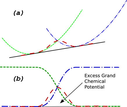
Figure 6: (Color Online) Illustration of the existence of an excess interface energy contribution from the chemical free energy. Upper panel: the concentration inside the interfacial region does not necessarily follow the common tangent line. Here, the two convex curves are the free energy densities of the individual phases in contact, the straight line is the common tangent, and the thick non-monotonous line is the concentration along a cut through the interface. Lower panel: the grand chemical potential in the interface differs from the one obtained by a weighted sum of the bulk phase free energies, where the weighting coefficients are the interpolating functions of the order parameters.

Therefore, there is a contribution to the surface free energy which is given by the following expressions. For binary eutectic systems ($N=3$ phases, $\mbox{\boldmath{$\phi$}}=\left(\phi_{\alpha},\phi_{\beta},\phi_{l}\right)$; $K=2$ components $\mbox{\boldmath{$c$}}=\left(c_{A},c_{B}\right)$), the vector $c$ is one-dimensional and we define the concentration ($c_{A}$) to be the independent field $\mbox{\boldmath{$c$}}=\left(c_{A},1-c_{A}\right)$. Then, we have

$${\Delta f}_{\textrm{chem}}\left(\mbox{\boldmath{$\phi$}},\mbox{\boldmath{$c$}};T\right)=f\left(\mbox{\boldmath{$\phi$}},\mbox{\boldmath{$c$}};T\right)-f_{l}-\mu_{A}(T)\left(c_{A}-c^{l}_{A}\right),$$ (56)

where $\mu_{A}\left(T\right)=\dfrac{\partial f\left(\mbox{\boldmath{$\phi$}},\mbox{\boldmath{$c$}};T\right)}{c_{A}}$ is the chemical potential of component A. For ternary eutectic systems ($N=4$ phases, $\mbox{\boldmath{$\phi$}}=\left(\phi_{\alpha},\phi_{\beta},\phi_{\gamma},\phi_{l}\right)$; $K=3$ components, $\mbox{\boldmath{$c$}}=\left(c_{A},c_{B},c_{C}\right)$), the vector $c$ is two-dimensional and with the concentrations of $A,B$ as the independent concentration fields, we get $\mbox{\boldmath{$c$}}=\left(c_{A},c_{B},1-c_{A}-c_{B}\right)$ and the chemical free energy excess becomes

$${\Delta f}_{\textrm{chem}}\left(\mbox{\boldmath{$\phi$}},\mbox{\boldmath{$c$}};T\right)=f\left(\mbox{\boldmath{$\phi$}},\mbox{\boldmath{$c$}};T\right)-f_{l}-\left(\mu_{A}(T)\right)\left(c_{A}-c^{l}_{A}\right)-\left(\mu_{B}\left(T\right)\right)\left(c_{B}-c^{l}_{B}\right).$$ (57)

The entire surface excess can thus be written as the following

$$\widetilde{\sigma}_{\alpha l} = \int_{x}\Big{(}T\epsilon a\left(\mbox{\boldmath{$\phi$}},\nabla\mbox{\boldmath{$\phi$}}\right)+\frac{T}{\epsilon}{w\left(\mbox{\boldmath{$\phi$}}\right)}+{\Delta f}_{\textrm{chem}}\left(\mbox{\boldmath{$\phi$}},\mbox{\boldmath{$c$}};T\right)\Big{)}dx$$ (58)

where $x$ is the coordinate normal to the interface, and the integral is taken along the equilibrium profile $\mbox{\boldmath{$\phi$}}(x)$, $\mbox{\boldmath{$c$}}(x)$. This integral cannot be calculated analytically. Therefore, we determine the surface free energy numerically. To this end, we perform one-dimensional simulations to determine the equilibrium profiles of concentration and phase fields, and insert the solution into the above formula to calculate $\tilde{\sigma}$. For these simulations, the known bulk values of the concentration fields are used as boundary conditions. To accurately calculate the surface excesses, it is important to include the contribution of the adsorbed phases. For this, the above calculations are performed by letting a small amount of these phases equilibrate at the interface of the major phases. Since the adsorbed phases equilibrate with very different concentrations compared to that of the bulk phases, the domain is chosen large enough such that the chemical potential change of the bulk phases during equilibration is kept negligibly low.

Another important quantity which is required as an input in the theoretical expressions is the latent heat of fusion $L^{\alpha}$ of the $\alpha$ phase. We follow the thermodynamic definition for the latent heat of transformation $L^{\alpha}$,

$$L^{\alpha} = T_{E}\left(s^{l}-s^{\alpha}\right),$$ (59)

$$\textrm{with}\hskip 7.11317pts = -\left(\dfrac{\partial f\left(\mbox{\boldmath{$\phi$}},\mbox{\boldmath{$c$}};T\right)}{\partial T}\right)$$ (60)

$$\textrm{and in particular}\hskip 7.11317pts^{l} = \sum_{i=1}^{K}c^{l}_{i}ln\left(c^{l}_{i}\right)$$ (61)

$$\textrm{and}\hskip 7.11317pts^{\alpha} = \sum_{i=1}^{K}c^{\alpha}_{i}\dfrac{L_{i}^{\alpha}}{T_{i}^{\alpha}}+c^{\alpha}_{i}ln\left(c^{\alpha}_{i}\right),$$ (62)

where the concentrations of the phases are taken from the phase diagram at the eutectic temperature.

Finally, let us give a few comments on the interface mobility $\mu_{\rm int}$ that appears in Eq. (4). In early works Caginalp and Xie (1993), it was shown that an expression for this mobility in terms of the phase-field parameters can be easily derived in the sharp-interface limit in which the interface thickness tends to zero. Later on, Karma and Rappel Karma and Rappel (1996) proposed the thin-interface limit, in which the interface width remains finite, but much smaller than the mesoscopic diffusion length of the problem. This limit relaxes some of the stringent requirements of the sharp-interface method for the achievement of quantitative simulations. Additionally, this method introduces a correction term to the original expression for the interface mobility, which makes it possible to carry out simulations in the vanishing interface kinetics (infinite interface mobility) regime.

Clearly, such modifications of the interface kinetics are also present in our model, where they arise both from the presence of adsorbed phases in the interface and from the structure of the concentration profile through the interface. Furthermore, it is well known that solute trapping also occurs in phase-field models of the type used here Ahmad et al. (1998). Since the interface profile can only be evaluated numerically, and since several phase-field and concentration variables need to be taken into account, it is not possible to evaluate quantitatively the contribution of these effects to the interface mobility. However, this lack of knowledge does not decisively impair the present study since we are mainly interested in undercooling versus spacing curves at a fixed interface velocity. At constant velocity, the absolute value of the interface undercooling contains an unknown contribution from the interface kinetics, but the relative comparison between steady states of different spacings remains meaningful. In addition, even though our simulation parameters correspond to higher growth velocities than typical experiments, it will be seen below that the value of the kinetic undercooling in our simulations is small. This indicates once more that our comparisons remain consistent.

IV Simulation results

In this section, we compare data extracted from phase-field simulations with the theory developed in Sec.II, for the case of coupled growth of the solid phases in directional solidification. The simulation setup is sketched in Figure 7.

Figure 7: Simulation setup for the phase-field simulations of binary and ternary eutectic systems. We impose a temperature gradient $G$ along the $z$ direction and move it with a fixed velocity. The average interface position follows the isotherms at steady state in case of stable lamellar coupled growth.

Periodic boundary conditions are used in the transverse direction, while no-flux boundary conditions are used in the growth direction. The box width in the transverse direction directly controls the spacing $\lambda$. The box length in the growth direction is chosen several times larger than the diffusion length. The diffusivity in the solid is assumed to be zero. A non-dimensional temperature gradient, G is imposed in the growth direction and moved with a velocity $v$, such that the temperature field is given by Eq. (48).

The outline of this section is as follows: first, we will briefly sketch how we extract the front undercooling from the simulation data. Then, this procedure will be validated by comparisons of the results to analytically known solutions as well as to data for binary alloys, for which well-established benchmark results exist. We start the presentation of our results on ternary eutectics by a detailed discussion of the two simplest possible cycles, $\alpha\beta\gamma$ and $\alpha\beta\alpha\gamma$. We compare the data for undercooling as a function of spacing to our analytical predictions and determine the relevant instabilities that limit the range of stable spacings. Finally, we also discuss the behavior of more complicated cycles, for sequences up to length $M=6$.

IV.1 Data extraction

At steady state, the interface velocity matches the velocity of the isotherms. The undercooling of the solid-liquid interface is extracted at this stage by the following procedure. First, a vertical line of grid points is scanned until the interface is located. Then, the precise position of the interface is determined as the position of the level line $\phi_{\alpha}=\phi_{\beta}$ for an $\alpha\beta$-interface (and in an analogous way for all the other interfaces). This is done by calculating the intersection of the phase-field profiles of the corresponding phases, which are extrapolated to subgrid accuracy by polynomial fits. In the presence of adsorbed phases at the interface, the two major phases along the scan line are used for determining the interface point. The major phases are determined from the maximum values that a particular order parameter assumes along the scan line. The temperature at a calculated interface point is then given by Eq. (48).

In order to test both our data extraction methods and our calculations of the surface tensions, we have performed the following consistency check. For an alloy with a symmetric phase diagram at the eutectic concentration, a lamellar front has an equilibrium position when a small temperature gradient ($G=0.001$) is applied to the system at zero growth speed. Since the concentration in the liquid is uniform for a motionless front, according to the Gibbs-Thomson relation the interface shapes should just be arcs of circles. This was indeed the case in our simulations, and the fit of the interface shapes with circles has allowed us to obtain the interface curvature and the contact angles with very good precision. The extraction of the data is illustrated in Figure 8.

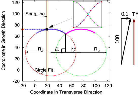
Figure 8: (Color Online) Procedure to extract the interface points from the simulation data with sub-grid resolution using higher order interpolation of the phase-field profiles. For the evaluation of the equilibrium properties, the solid-liquid interface points of each lamella are fitted with a circle which is then used to measure the radius of curvature of the particular lamella. We also calculate the triple point angles as the angles between the tangents to the circles at one of the points of intersection.

We fit the radius and the coordinates of the circle centers. Then, the angle at the trijunction point $\theta$ is deduced from geometrical relations, with $d=a+b$ and $a=\dfrac{R_{a}^{2}-R_{b}^{2}+d^{2}}{2d}$,

$$b=d-a$$

$$\theta=\cos^{-1}\left(\dfrac{a}{R_{a}}\right)+\cos^{-1}\left(\dfrac{b}{R_{b}}\right).$$

The meaning of the lengths $a$ and $b$ is given in Figure 8.

IV.2 Validation: Binary Systems

For comparison with the $\Delta T-\lambda$ relationship known from Jackson-Hunt(JH) theory, we create two binary eutectic systems by choosing suitable parameters $L_{i}^{\alpha}$ and $T_{i}^{\alpha}$ in the free energy density $f\left(\mbox{\boldmath{$\phi$}},\mbox{\boldmath{$c$}};T\right)$. A symmetric binary eutectic system, shown in Figure 9, is created by

$$L_{i}^{\alpha}=\left(\begin{array}[]{lll}&A&B\\ \alpha&4.0&4.0\\ \beta&4.0&4.0\end{array}\right)$$

$$T_{i}^{\alpha}=\left(\begin{array}[]{lll}&A&B\\ \alpha&1.0&0.75980\\ \beta&0.75980&1.0\end{array}\right).$$

Figure 9: Binary eutectic phase diagrams for a model system with stable (solid lines) and metastable (light dashed lines) extensions of the solidus and the liquidus lines, of (a) a symmetric A-B and (b) an unsymmetric C-D system.

To create an asymmetric binary eutectic system, shown in Figure 9, we choose

$$L_{i}^{\alpha}=\left(\begin{array}[]{lll}&C&D\\ \alpha&5.0&5.0\\ \beta&5.0&5.0\end{array}\right)$$

$$T_{i}^{\alpha}=\left(\begin{array}[]{lll}&C&D\\ \alpha&0.96&0.80137\\ \beta&0.76567&1.0\end{array}\right)$$

The numbers $L_{i}^{\alpha}$, $T_{i}^{\alpha}$ are chosen such that the widths of each of the (lens-shaped) two-phase coexistence regions remain reasonably broad, and that the approximation of using the values of concentration difference between the solidus and liquidus $\left(\Delta c_{\nu}^{l}\right)$ at the eutectic temperature for the theoretical expressions holds for a good range of undercoolings. This implies that the value of the $L_{i}^{\alpha}$ should not be too small. Conversely, a too high value is also not desirable since for large values of $L_{i}^{\alpha}$ the chemical contribution to the surface free energy becomes large, which leads to very steep and narrow interface profiles.

Table 1: Parameters for the sharp-interface theory, with proper calculation of the surface tension in the phase-field simulations for (a) a symmetric binary eutectic system with components A and B and (b) for an unsymmetric binary eutectic system with components C and D.

(a) $\widetilde{\sigma}_{\alpha l}$ 1.01146 $\widetilde{\sigma}_{\beta l}$ 1.01146 $\widetilde{\sigma}_{\alpha\beta}$ 1.23718 $\theta_{\alpha\beta}$ 37.70 $\theta_{\beta\alpha}$ 37.70 $L^{\alpha}$ 4.0 $L^{\beta}$ 4.0 $m_{B}^{\alpha}=m_{A}^{\beta}$ -0.206975     (b) $\widetilde{\sigma}_{\alpha l}$ 0.97272 $\widetilde{\sigma}_{\beta l}$ 1.07235 $\widetilde{\sigma}_{\alpha\beta}$ 1.24836 $\theta_{\alpha\beta}$ 33.903 $\theta_{\beta\alpha}$ 41.161 $L^{\alpha}$ 4.686 $L^{\beta}$ 4.711 $m_{D}^{\alpha}$ -0.13161 $m_{C}^{\beta}$ -0.22138

We perform simulations at two different velocities V = 0.01 and V = 0.02, with a mesh size $\Delta x=1.0$ and the parameter set $\epsilon=4.0,D^{l}_{A}=D^{l}_{B}=D^{l}_{C}=D^{l}_{D}=1.0,\sigma_{\alpha\beta}=\sigma_{\alpha l}=\sigma_{\beta l}=1.0,\sigma_{\alpha\beta\gamma}=10.0$. To give an idea of the order of magnitude of the corresponding dimensional quantities, we remark that if we assume the melting temperatures to be around 1700K and the other values to correspond to the Ni-Cu system used in the study of Warren et al. Warren and Boettinger (1995), the length scale $d^{*}$ for the case of the binary eutectic system turns out to be around 0.2 nm and the time scale 0.04 ns.

The corresponding parameters for the sharp-interface theory are given in Table 1. The comparisons between our numerical results and the analytic theory are shown in Figs. 10 and 10.

Figure 10: Comparison of $\Delta T-\lambda$ relations resulting from the theoretical analysis and from the phase-field simulations at two different velocities for systems; (a) symmetric binary eutectic system (A-B) and (b) unsymmetric binary eutectic system (C-D).

Consistent differences can be observed in the undercooling values between our data and the predictions from JH theory for both systems. The difference in undercoolings is smaller at lower velocities, which hints at the presence of interface kinetics. We find indeed that when we change the relaxation constant in the phase-field evolution equation by about 50 %, the difference between the predicted and measured undercoolings is removed for the case of the considered symmetric binary phase diagram. This clearly shows that the interface kinetics is not negligible. It seems difficult, however, to obtain a precise numerical value for its magnitude in the framework of the present model.

The spacing at minimum undercooling, however, is reproduced to a good degree of accuracy (error of 5 %), while the minimum undercooling has a maximum error of 10 %. It should also be noted that the JH theory only is an approximation for the true front undercooling. Results obtained both with boundary integral Karma and Sarkissian (1996) and quantitative phase-field methods Folch and Plapp (2005) have shown that, whereas the prediction for the minimum undercooling spacing is excellent, errors of 10 % for the value of the undercooling itself are typical. If the JH curve is drawn without taking into account the additional chemical contributions to the surface tension, a completely different result is obtained, with minimum undercooling spacings that are largely different from the simulated ones. We can therefore conclude that we have captured the principal corrections.

In addition, we have performed equilibrium measurements of the angles at the trijunction point and of the radius of curvature of the lamellae as described in the preceding sub-section (IV.1) for the symmetric eutectic system. The contact angles differ from the ones predicted by Young’s equilibrium conditions only by a value of 0.2 degrees. The theoretical (from the Gibbs-Thomson equation) and measured undercoolings differ in the third decimal, with an error of 0.1 %.

IV.3 Ternary Systems: Parameter set

$$L_{i}^{\alpha}=\left(\begin{array}[]{llll}&A&B&C\\ \alpha&1.46964038&1.0&1.0\\ \beta&1.0&1.46964038&1.0\\ \gamma&1.0&1.0&1.46964038\end{array}\right)$$

$$T_{i}^{\alpha}=\left(\begin{array}[]{llll}&A&B&C\\ \alpha&1.5&0.5&0.5\\ \beta&0.5&1.5&0.5\\ \gamma&0.5&1.0&1.5\end{array}\right).$$

We use a symmetric ternary phase diagram. The following matrices list the parameters $L_{i}^{\alpha}$,$T_{i}^{\alpha}$ in the free energy $f\left(\mbox{\boldmath{$\phi$}},\mbox{\boldmath{$c$}};T\right)$ that were used to create a symmetric ternary eutectic system, shown in Figure 1. We perform simulations with the parameter set $\epsilon=8.0,\Delta x=1.0,D^{l}_{A}=D^{l}_{B}=D^{l}_{C}=1.0,\sigma_{\alpha\gamma}=\sigma_{\beta\gamma}=\sigma_{\gamma\beta}=\sigma_{\alpha l}=\sigma_{\beta l}=\sigma_{\gamma l}=1.0,\sigma_{\alpha\beta l}=\sigma_{\alpha\beta\gamma}=\sigma_{\alpha\gamma l}=\sigma_{\beta\gamma l}=10.0$ and compare with the theoretical expressions using the input parameters listed in Table 2.

Table 2: Input parameters for the theoretical relations for the ternary eutectic system.

$\widetilde{\sigma}_{\alpha l}=\widetilde{\sigma}_{\beta l}=\widetilde{\sigma}_{\gamma l}$	1.194035
$\widetilde{\sigma}_{\alpha\beta}=\widetilde{\sigma}_{\alpha\gamma}=\widetilde{\sigma}_{\beta\gamma}$	1.430923
$\theta_{\alpha\beta}=\theta_{\beta\alpha}=\theta_{\gamma\alpha}$ = $\theta_{\alpha\gamma}$	36.81
$L^{\alpha}=L^{\beta}=L^{\gamma}$	1.33
$m_{B}^{\alpha}=m_{C}^{\alpha}$	-0.91
$m_{A}^{\beta}=m_{C}^{\beta}$	-0.91
$m_{A}^{\gamma}=m_{B}^{\gamma}$	-0.91

IV.4 Simple cycles: steady states and oscillatory instability

We first perform simulations to isolate the regime of stable lamellar growth for the configuration $\alpha\beta\gamma$. For this regime, we measure the average interface undercooling and compare it to our theoretical predictions. The results are shown in Figure 11.

Figure 11: Comparison between theoretical analysis and phase-field simulations at two different velocities for the arrangement $\left(\alpha\beta\gamma\right)$ of ternary eutectic solids at $V=0.005$ and $V=0.01$. The demarcation shows the regions of stable lamellar growth and the critical spacing beyond which we observe amplified oscillatory behavior. There is a small region named “Damped Oscillations”, which is a region where oscillations occur but die down slowly with time.

The agreement in the undercoolings is much better than for the binary eutectic systems, with a smaller dependence of undercoolings on the velocities. Consequently, both the spacing at minimum undercooling (error  4 % for V=0.005 and  6 % for V=0.01) and the minimum undercooling (error of 1-2 %), match very well with the theoretical relationships, as shown in Figure 11. The equilibrium angles at the triple point also agree with the ones predicted from Young’s law to within an error of 0.3 degrees, while the radius of curvature matches that from the Gibbs-Thomson relationship with negligible error (<0.5 %).

It should be noted that the steady lamellae remain straight, contrary to the results of Ref. Hecht et al. (2004), where a spontaneous tilt of the lamellae with respect to the direction of the temperature gradient was reported. This difference is due to the different phase diagrams: we are using a completely symmetric phase diagram and equal surface tensions for all solid-liquid interfaces, whereas Hecht et al. (2004) uses the thermophysical data of a real alloy.

Next, we are interested in the stability range of three-phase coupled growth. From general arguments, we expect a long-wavelength lamella elimination instability (Eckhaus-type instability) to occur for low spacings, as in binary eutectics Akamatsu et al. (2004b). Here, we will focus on oscillatory instabilities that occur for large spacings. It is useful to first recall a few facts known about binary eutectics, where all the instability modes have been classified Karma and Sarkissian (1996); Ginibre et al. (1997). Lamellar arrays in binary eutectics are characterized (in the absence of crystalline anisotropy) by the presence of two mirror symmetry planes that run in the center of each type of lamellae, as sketched in Figure 12(a). Instabilities can break certain of these symmetries while other symmetry elements remain intact Coullet and Iooss (1990). In binary eutectics, the oscillatory 1-$\lambda$-O mode is characterized by an in-phase oscillation of the thickness of all $\alpha$ (and $\beta$) lamellae; both mirror symmetry planes remain in the oscillatory pattern. In contrast, in the 2-$\lambda$-O mode, one type of lamellae start to oscillate laterally, whereas the mirror plane in the other type of lamellae survives; this leads to a spatial period doubling. Finally, in the tilted pattern both mirror planes are lost.

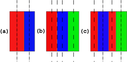
Figure 12: (Color Online) In a periodic arrangement of lamellae, we can identify certain lines of symmetry, as shown in (a) for a binary eutectic. Similarly, for the case of the two simplest configurations, (b) $\alpha\beta\gamma$ and (c) $\alpha\beta\alpha\gamma$ in a symmetric ternary eutectic system, such planes of symmetry exist. While in the case of a binary eutectic, the lines are mirror symmetry axes (shown by dash-dotted lines), in the special case of a symmetric ternary phase diagram, one can also identify quasi-mirror lines (dashed lines) where we retrieve the original configuration after a spatial reflection and an exchange of two phases. Only quasi-mirror lines exist in the $\alpha\beta\gamma$ arrangement, which are shown in (b), while both true- and quasi-mirror planes exist in the $\alpha\beta\alpha\gamma$ arrangement as shown in (c).

It is therefore important to survey the possible symmetry elements in the ternary case. At first glance, there seems to be no symmetry plane in the pattern. However, for our specific choice of phase diagram, new symmetry elements not present in a generic phase diagram exist: mirror symmetry planes combined with the exchange of two phases. Consider for example the $\beta$ phase in the center of Figure 12(b): if the system is reflected at its center, and then the $\alpha$ and $\gamma$ phases are exchanged, we recover the original pattern. At the eutectic concentration, there are three such symmetry planes running in the center of each lamella, and three additional ones running along the three solid-solid interfaces. Off the eutectic point, two of these planes survive if any two of the three phases have equal volume fractions.

Guided by these considerations, we can conjecture that there are two obvious possible instability modes, sketched in Figure 13.

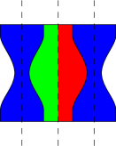
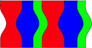
Figure 13: (Color Online) Guided by the symmetry axes in the $\alpha\beta\gamma$ arrangement, one can expect two possible oscillatory modes at off-eutectic concentrations along the eutectic groove. The oscillations in (a), which keep all the quasi-mirror planes intact, are expected to occur at concentrations towards the apex of the simplex along the eutectic groove. Another possibility, shown in (b) exists in which no symmetry plane remains, which is expected to occur at a concentration towards the binary edge of the simplex.

In the first, called mode 1 in the following, two symmetry planes survive: the width of one lamella oscillates, whereas the two other phases form a “composite lamella” that oscillates in opposition of phase; the interface in the center of this composite lamella does not oscillate at all and constitutes one of the symmetry planes. In the second (mode 2), the lateral position of one of the lamellae oscillates with time, whereas the other two phases oscillate in opposition of phase to form a “composite lamella” that oscillates laterally but keeps an almost constant width. There is no symmetry plane left in this mode.

The stability range of the coupled growth regime of the lamellar arrangement is indicated in Figure 11. Steady lamellar growth is stable from below the minimum undercooling spacing up to a point where an oscillatory instability occurs. In the region marked “damped oscillations”, oscillatory motion of the interfaces was noticed, but died out with time. Above a threshold in spacing, oscillations are amplified. We monitored the modes that emerged, and found indeed good examples for the two theoretically expected patterns, shown in Figure 14.

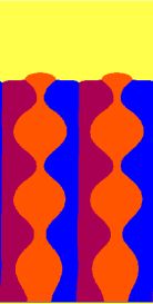
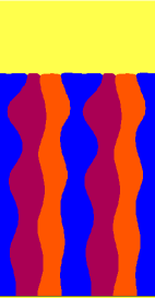
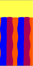
Figure 14: (Color Online) Oscillatory modes in simulations for the $\alpha\beta\gamma$ configuration at the off-eutectic concentrations $\mbox{\boldmath{$c$}}=\left(0.32,0.32,0.36)\right)$ in (a), and $\mbox{\boldmath{$c$}}=\left(0.34,0.34,0.32\right)$ in (b) and (c). The spacings are $\lambda=170$ in (a) and (c) and $\lambda=165$ in (b).

Mode 1 is favored for off-eutectic concentrations in which one of the lamellae is wider than the two others, such as $\mbox{\boldmath{$c$}}=(0.32,0.32,0.36)$. Indeed, in that case the (unstable) steady-state pattern exhibits the same symmetry planes as the oscillatory pattern. This mode can also appear when one lamella is smaller than the two others, see Figure 14. We detect mode 2 at the eutectic concentration, see Figure 15. However, a “mixed mode” can also occur, in which no symmetry plane survives, but the three trijunctions oscillate laterally with phase differences that depend on the concentration and possibly on the spacing, see Figs. 14 and 15.

Figure 15: The plot shows the trace of the triple points for the $\alpha\beta\gamma$ arrangement. The growth direction is compressed in these plots with respect to the transverse direction in order to better visualize the modes. We get multiple modes at the eutectic concentration for the same spacing $\lambda=159$, shown in (a) and (b). In (a) we get back mode 1 while (b) matches well to our predicted mode 2. A mixed mode (c) is obtained at an off-eutectic concentration $\mbox{\boldmath{$c$}}=\left(0.34,0.34,0.32\right)$, at a spacing $\lambda=165$, which is a combination of oscillations in both the width and lateral spacing.

Figure 16: Theoretical analysis and phase-field simulations: Comparison between the arrangements $\left(\alpha\beta\gamma\right)$ and $\left(\alpha\beta\alpha\gamma\right)$ for two different velocities (a) V = 0.005 and (b) V = 0.01. Plots convey information on the stability ranges, and the onset of oscillatory behavior of the 1-$\lambda$-O type.

Let us now turn to the $\alpha\beta\alpha\gamma$ cycle. We perform simulations for two different velocities $V=0.01$ and $V=0.005$. The comparison of the measurements with the theoretical analysis for steady-state growth is shown in Figure 16. For the purpose of analysis, predictions from the theory for both arrangements ($\alpha\beta\gamma$ and $\alpha\beta\alpha\gamma$) are also shown. Here again, the minimum undercooling spacings match those of the theory to a good degree of accuracy (error  5%, V=0.005). However, the undercooling is lower than the one predicted by JH-theory, with a discrepancy of 4% for the case of $V=0.005$, Figure 16. For $V=0.01$, Figure 16, simulations were not possible for a sufficient range of $\lambda$ to determine the minimum undercooling, because the width of the narrowest lamellae became comparable to the interface width $\epsilon\simeq 8.0$ before the minimum was reached. However, the general trend of the data follows the predictions of the theory for both velocities. This was also the case for simulations carried out at an off-eutectic concentration $\mbox{\boldmath{$c$}}=(0.32,0.34,0.34)$ at a velocity of $V=0.005$, for the same configuration $\alpha\beta\alpha\gamma$.

Concerning the oscillatory instabilities at large spacings, it is useful to consider again the symmetry elements. For this cycle, there are two real symmetry planes in the steady-state pattern that run through the centers of the $\beta$ and $\gamma$ lamellae. Note that these symmetries would exist even for unsymmetric phase diagrams and unequal surface tensions. Therefore, by analogy with binary eutectics, one may expect oscillatory modes that simply generalize the 1-$\lambda$-O and 2-$\lambda$-O modes of binary eutectics, see Figure 17. Indeed, for our simulations at the eutectic concentration, we retrieve the 1-$\lambda$-O type oscillation, figure 18 as in our hypothesis (figure 17).

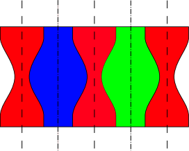
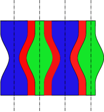
Figure 17: (Color Online) Predictions of oscillatory modes for the $\alpha\beta\alpha\gamma$ arrangement, reminiscent of the 1-$\lambda$-O mode (a) and 2-$\lambda$-O mode (b) in binary eutectics.

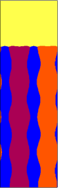
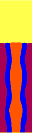
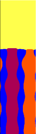
Figure 18: (Color Online) Simulations of oscillatory modes of the $\alpha\beta\alpha\gamma$ configuration. The modes in (a) and (b) show resemblance to the 1-$\lambda$-O and 2-$\lambda$-O oscillatory modes of binary eutectics, respectively. Additionally, other modes (c) can also be observed, depending on the initial conditions. While we observe (a) at the eutectic concentration, (b) and (c) are modes at off-eutectic concentrations $\mbox{\boldmath{$c$}}=(0.32,0.34,0.34)$. The spacings are (a) $\lambda=201$, (b) $\lambda=174$ (c) $\lambda=210$.

This oscillatory instability can be quantitatively monitored by following the lateral positions of the solid-solid interfaces with time. More specifically, we extract the width of the $\beta$ phase as a function of the growth distance $z$. This is then fitted with a damped sinusoidal wave of the type $A_{0}+A\exp(-Bz)\cos((2\pi z/L)+D)$. The damping coefficient $B$ is obtained from a curve fit and plotted as a function of the spacing $\lambda$. The onset of the instability is characterized by the change in sign of the damping coefficient.

For the off-eutectic concentration we get two modes (figure 18). While (figure 18) corresponds well to our hypothesis to the 2-$\lambda$-O type oscillation (figure 17), we also observe another mode as shown in figure 18, which combines elements of the two modes: both the width and the lateral position of the $\alpha$ lamellae oscillate.

IV.5 Lamella elimination instability

For the $\alpha\beta\alpha\gamma$ cycle, there is also a new instability, which occurs for low spacings. We find that all spacings below the minimum undercooling spacing, as well as some spacings above it, are unstable with respect to lamella elimination: the system evolves to the $\alpha\beta\gamma$ arrangement by eliminating one of the $\alpha$ lamellae, both at eutectic and off-eutectic concentrations. The points plotted to the left of the minimum in Figure 16 are actually unstable steady states that can be reached only when the simulation is started with strictly symmetric initial conditions and the correct volume fractions of the solid phases.

This instability can actually be well understood using our theoretical expressions. As already mentioned before, when we consider the cycle $\alpha\beta\alpha\gamma$ at the eutectic concentration with a lamella width configuration $(\xi,1/3,1/3-\xi,1/3)$, the global average front undercooling attains a minimum for the symmetric pattern $\xi=1/6$. However, the global front undercooling is not the most relevant information for assessing the front stability. More interesting is the undercooling of an individual lamella, because this can give information about its evolution. More precisely, consider the undercooling of one of the $\alpha$ lamellae as a function of $\xi$. If the undercooling increases when the lamella gets thinner, then the lamella will fall further behind the front and will eventually be eliminated. In contrast, if the undercooling decreases when the lamella gets thinner, then the lamella will grow ahead of the main front and get larger. A similar argument has been used by Jackson and Hunt for their explanation of the long-wavelength elimination instability Jackson and Hunt (1966). It should be pointed out that the new instability found here is not a long-wavelength instability, since it can occur even when only one unit cell of the cycle is simulated.

Following the above arguments, we have calculated the growth temperature of the first $\alpha$ lamella as a function of $\xi$ using the general expressions in Eq. 33. In Figure 19, we plot the variation of $\partial\Delta T/\partial\xi$ at $\xi=1/6$, as a function of $\lambda$. The point at which $\partial\Delta T/\partial\xi$ becomes positive then indicates the transition to a stable $\alpha\beta\alpha\gamma$ cycle. This criterion is in good agreement with our simulation results. This argument can also be generalized to more complicated cycles (see below).

Figure 19: Plot of $\partial\Delta T/\partial\xi$, taken at $\xi=1/6$ versus $\lambda$ for the $\alpha_{1}\beta\alpha_{2}\gamma$ cycle, where $\Delta T$ is the undercooling of the $\alpha_{1}$ lamella and $\xi$ its width (relative to $\lambda$), calculated by our analytical expressions in the volume fraction configuration. $(\xi,1/3,1/3-\xi,1/3)$ at V=0.01. The cycle is predicted to be unstable to lamella elimination if $\partial\Delta T/\partial\xi<0$. The $\lambda$ at which $\partial\Delta T/\partial\xi$ changes sign is the critical point beyond which the $\alpha\beta\alpha\gamma$ arrangement is stable with respect to a change to the sequence $\alpha\beta\gamma$ through a lamella elimination.

IV.6 Longer cycles

Let us now discuss a few more complicated cycles. The simple cycles we have simulated until now were such that during stable coupled growth the widths of all the lamellae corresponding to a particular phase were the same. This changes starting from period $M=5$, where the configuration $\alpha\beta\alpha\beta\gamma$ is the only possibility (up to permutations). If we consider this cycle at the eutectic concentration and note the configuration of lamella widths as $(\xi,1/3-\xi,1/3-\xi,\xi,1/3)$ and compute the average front undercooling by our theoretical expressions, we find that the minimum occurs for $\xi$ close to $0.12$. In addition, for this configuration, the undercooling of any asymmetric configuration (permutation of widths of lamellae) is higher than the one considered above. If we rewrite symbolically this configuration as $\alpha_{1},\beta_{2},\alpha_{2},\beta_{1},\gamma$, it is easy to see that this configuration has two symmetry axes of the same kind as discussed in the preceding subsection: mirror reflection and exchange of the phases $\alpha$ and $\beta$. One of them runs along the interface between $\beta_{2}$ and $\alpha_{2}$, and the other one in the center of the $\gamma$ lamella.

Not surprisingly, our simulation results confirm the importance of this symmetry. The volume fractions in steady-state growth are close to those that give the minimum average front undercooling, see Figs. 20 and 20.

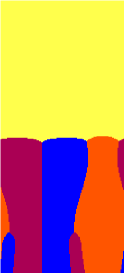
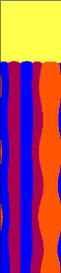
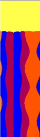
Figure 20: (Color Online) Simulations at spacings $\lambda=135$ in (a), $\lambda=150$ in (b) and $\lambda=180$ in (c), starting from an initial configuration of $\alpha\beta\alpha\beta\gamma$. There is no spacing for which the $\alpha\beta\alpha\beta\gamma$ develops into a stable lamellar growth front. Smaller spacings switch to the $\alpha\beta\gamma$ arrangement while the larger spacings exhibit oscillatory instabilities in both the width and the lateral positions of the lamellae.

Additionally, we observe oscillations in the width of the largest $\gamma$ phase and oscillations in the widths and the lateral position of the smaller lamellae of the $\alpha$ and $\beta$ phases, while the interface between the larger $\alpha$ and $\beta$ phase remains straight, such that the combination of all the $\alpha$ and $\beta$ lamellae oscillates in width as one “composite lamella”. Thus, the symmetry elements of the underlying steady state are preserved in the oscillatory state.

For smaller spacings, this configuration is unstable, and the sequence changes to the $\beta\alpha\gamma$ arrangement as shown in Figure 20 by two successive lamella eliminations. It is noteworthy that we did not find any unstable sequence which switches to the $\alpha\beta\alpha\gamma$ arrangement, which again can be understood from the presence of the symmetry. Indeed, a symmetrical evolution would result in a change to a configuration $\alpha_{1}\beta_{1}\gamma$ or $\beta_{2}\alpha_{2}\gamma$, but precludes the change to a configuration of period length $M=4$.

Going on to cycles with period $M=6$, the first arrangement we consider is $\alpha_{1}\beta_{1}\alpha_{2}\beta_{2}\alpha_{1}\gamma$, where we name the lamellae for eventual discussion and ease in description according to the symmetries. Indeed, this arrangement has two exact mirror symmetry planes in the center of the $\alpha_{2}$ and the $\gamma$ phases. We find that, if we calculate the average interface undercooling curves by varying the widths of individual lamella with the constraint of constant volume fraction, by choosing different $\xi$, in the width configuration $(\xi,1/6,1/3-2\xi,1/6,\xi,1/3)$, the average undercooling at the growth interface is minimal for the configuration $(1/9,1/6,1/9,1/6,1/9,1/3)$. This arrangement has the highest undercooling curve among the arrangements we have considered, shown in Figure 21.

Figure 21: (a)Synopsis of the theoretical predictions for the undercooling versus spacing of possible arrangements between period length $M=3$ to $M=6$, i.e. starting from $\alpha\beta\gamma$ to $\alpha\beta\gamma\alpha\beta\gamma$. (b) Same plot but with the lamellar repeat distance $\lambda$ scaled with the period length M. The variation among the arrangements is purely a result of the variation of the solutal undercooling as can be infered from the discussion in Sec. II.4.

It also has a very narrow range of stability, and we could isolate only one spacing which exhibits stable growth for $\lambda=240$, Figure 22. Unstable arrangements near the minimum undercooling spacing evolve to the $\alpha\beta\gamma$ arrangement, Figure 22, while for other unstable configurations we obtain the arrangements in Figure 22 and Figure 22 as the stable growth forms corresponding to $\lambda=150$ and $\lambda=180$ respectively.

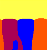
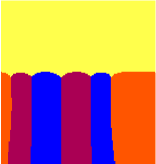
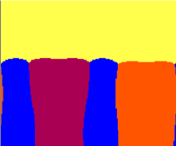
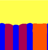
Figure 22: (Color Online) Simulations starting from the arrangement $\alpha\beta\alpha\beta\alpha\gamma$ for spacings $\lambda=135$ in a), $\lambda=150$ in b), $\lambda=180$ in c) and $\lambda=240$ in d).

Apart from the (trivial) period-doubled arrangement $\alpha\beta\gamma\alpha\beta\gamma$, another possibility for $M=6$ is $\alpha\beta\gamma\alpha\gamma\beta$ with a volume fraction configuration $(1/6,1/6,1/6,1/6,1/6,1/6)$. Simulations of this arrangement show that there exists a reasonably large range of stable lamellar growth, and hence we could make a comparison between simulations and the theory. We find similar agreement between our measurements and theory as we did previously for the arrangements $\alpha\beta\gamma$ and $\alpha\beta\alpha\gamma$. The plot in Figure 21 shows the theoretical predictions of all the arrangements we have considered until now.

IV.7 Discussion

It should by now have become clear that there exists a large number of distinct steady-state solution branches, each of which can exhibit specific instabilities. In addition, the stability thresholds potentially depend on a large number of parameters: the phase diagram data (liquidus slopes, coexistence concentration), the surface tensions (assumed identical here), and the sample concentration. Therefore, the calculation of a complete stability diagram that would generalize the one for binary eutectics of Ref. Karma and Sarkissian (1996) represents a formidable task that is outside the scope of the present paper. Nevertheless, we can deduce from our simulations a few guidelines that can be useful for future investigation.

Lamellar steady-state solutions can be grouped into three classes, which respectively have (I) equal number of lamellae of all three phases (such as $\alpha\beta\gamma$ and $\alpha\beta\gamma\alpha\gamma\beta$), (II) equal number of lamellae for two phases (such as $\alpha\beta\alpha\gamma$), and (III) different numbers of lamellae for each phase.

For equal global volume fractions of each phase (as in most of our simulations), class III will have the narrowest stability ranges because of the simultaneous presence of very large and very thin lamella in the same arrangement, which make these patterns prone to both oscillatory and lamella elimination instabilities.

Any cycle in which a phase appears more than once can transit to another, simpler one by eliminating one lamella of this phase. This lamella instability always appears for low spacings below a critical value of the spacing that depends on the cycle. The possibility of a transition, however, depends also on the symmetries of the pattern. For instance, the arrangement $\alpha\beta\alpha\beta\alpha\gamma$, if unstable, can transform into the $\alpha\beta\gamma$, $\alpha\beta\alpha\gamma$ or the $\alpha\beta\alpha\beta\gamma$ arrangements, while for an arrangement $\alpha\beta\alpha\beta\gamma$, it is impossible to evolve into the $\alpha\beta\alpha\gamma$ arrangement if the symmetry of the pattern is preserved by the dynamics.

For large spacings, oscillatory instabilities occur and can lead to the emergence of saturated oscillatory patterns of various structures. The symmetries of the steady states seem to determine the structure of these oscillations, but no thorough survey of all possible nonlinear states was carried out.

V Some remarks on pattern selection

Up to now, we have investigated various regular periodic patterns and their instabilities. The question which, if any, of these different arrangements, is favored for given growth conditions, is still open. From the results presented above, we can already conclude that this question cannot be answered solely on the basis of the undercooling-vs-spacing curves. Indeed, we have shown that by appropriately choosing the initial conditions, any stable configuration can be reached, regardless of its undercooling. This is also consistent with experiments and simulations on binary eutectics Ginibre et al. (1997); Parisi and Plapp (2010). To get some additional insights on what happens in extended systems, we conducted some simulations of isothermal solidification where the initial condition was a random lamellar arrangement. More precisely, we initialize a large system with lamellae of width $\lambda=25$ and choose a random sequence of phases such that two neighboring lamellae are of different phases as shown in Figure 23. The global probabilities of all the phases are $1/3$, which corresponds to the eutectic concentration, and the temperature is set to $T=0.785$.

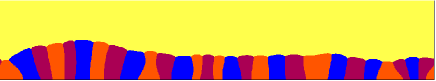
Figure 23: (Color Online) Two snapshots of 2D dynamics in a large system. Isothermal simulations are started from a random configuration in (a) where the probability of occurrence of each phase is $1/3$, which is also the global concentration in the liquid. The temperature of the system is T=0.785 and the concentration of the liquid is the eutectic concentration. A slowly changing pattern with a non-planar front is achieved. Some lamellae are eliminated, but no new lamellae are created.

Under isothermal growth conditions, one would expect that, at a given undercooling, the arrangement with highest local velocity would be the one that is chosen. However, in order for the front to adopt this pattern, a rearrangement of the phase sequence is necessary. In our simulations, we find that lamella elimination was possible (and indeed readily occurred). In contrast, there is no mechanism for the creation of new lamellae in our model, since we did not include fluctuations that could lead to nucleation, and the model has no spinodal decomposition that could lead to the spontaneous formation of new lamellae, as in Ref. Plapp and Karma (2002). As a result, some of the lamellae became very large in our simulations, which led to a non-planar growth front, as shown in Figure 23. No clearcut periodic pattern emerged, such that our results remain inconclusive.

We believe that lamella creation is an important mechanism required for pattern adjustment. In 2D, nucleation is the only possibility for the creation of new lamellae. In contrast, in 3D, new lamellae can also form by branching mechanisms without nucleation events, since there are far more geometrical possibilities for two-phase arrangements Akamatsu et al. (2001); Walker et al. (2007). Therefore, we also conducted a few preliminary simulations in 3D.

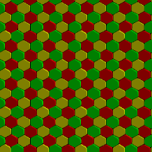
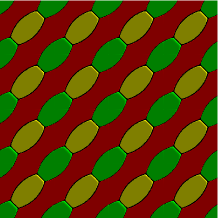
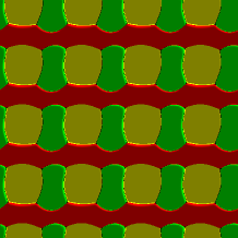
Figure 24: (Color Online) Cross-sections of patterns obtained in three-dimensional directional solidification. In each picture, the simulation unit cell is tiled in a 4$\times$4 array to get a better view of the pattern. The pattern in (a) was started from a random configuration and evolved to a perfectly hexagonal pattern (at the eutectic composition for a symmetric phase diagram). At an off-eutectic concentration, starting with two isolated rods of $\alpha$ and $\beta$ phase, the result shown in (b) is one of the possible structures, while with an asymmetric phase diagram at the eutectic concentration, we get a regular brick structure (c) from a random initial condition.

The cross sections of the simulated systems are $150\times 150$ grid points for results in Figs. 24(a) and (c), and $90\times 90$ grid points for the system Figure 24(b). The longest run took about 7 weeks on 80 processors, for the simulation of the pattern in Figure 24(a). This long simulation time is due to the fact that the pattern actually takes a long time to settle down to a steady state; the total solidification distance was of the order of 800 grid points. The other simulations required less time to reach reasonably steady states. The patterns shown in Figs. 24 (a) and (c) start from random initial conditions (very thin rods of randomly assigned phases), the former with the symmetric phase diagram used previously, the latter with a slightly asymmetric phase diagram constructed with the changed parameters listed below, $$L_{i}^{\alpha}=\left(\begin{array}[]{llll}&A&B&C\\ \alpha&2.0&1.0&1.0\\ \beta&1.0&2.0&1.0\\ \gamma&1.0&1.0&2.0\end{array}\right)$$ $$T_{i}^{\alpha}=\left(\begin{array}[]{llll}&A&B&C\\ \alpha&1.0&0.59534&0.63461\\ \beta&0.59534&1.0&0.63461\\ \gamma&0.59534&0.59534&1.0\end{array}\right).$$

The picture of Figure 24(b) corresponds to a pattern resulting of a simulation which is started with two isolated rods of $\alpha$ and $\beta$ in a matrix of $\gamma$, with an off-eutectic concentration of $\mbox{\boldmath{$c$}}=(0.3,0.4,0.3)$.

As shown in Figure 24, many different steady-state patterns are possible in 3D. Not surprisingly, the type of pattern seen in the simulations depends on the concentration and on the phase diagram. Patterns very similar to Figure 24(c) have recently been observed in experiments in the Al-Ag-Cu ternary system Ratke (2010). It should be stressed that our pictures have been created by repeating the simulation cell four times in each direction in order to get a clearer view of the pattern. This means that in a larger system, the patterns might be less regular. Furthermore, we certainly have not exhausted all possible patterns. A more thorough investigation of the 3D patterns and their range of stability is left as a subject for future work.

VI Conclusion and outlook

In this paper, we have generalized a Jackson-Hunt analysis for arbitrary periodic lamellar three-phase arrays in thin samples, and used 2D phase-field simulations to test our predictions for the minimum undercooling spacings of the various arrangements. For the model used here the value of the interface kinetic coefficient cannot be determined, which leads to some incertitude on the values of the undercooling, but this does not influence our principal findings. When the correct values of the surface free energy (that take into account additional contributions coming from the chemical part of the free energy density) are used for the comparisons with the theory, we find good agreement for the minimum undercooling spacings for all cycles investigated. Moreover, we find that, as in binary eutectics, all cycles exhibit oscillatory instabilities for spacings larger than some critical spacing. The type of oscillatory modes that are possible are determined by the set of symmetry elements of the underlying steady state.

We have repeatedly made use of symmetry arguments for a classification of the oscillatory modes. In certain cases, the symmetry is exact and general, which implies that the corresponding modes should exist for arbitrary phase diagrams and thus be observable in experiments. For instance, the mirror symmetry lines in the middle of the $\alpha$ lamellae in the $\alpha\beta\alpha\gamma$ arrangement exist even for non-symmetric phase diagrams and unequal surface tensions, and hence the corresponding oscillatory patterns and their symmetries should be universal. In other cases, we have used a symmetry element which is specific to the phase diagram used in our simulations: a mirror reflection, followed by an exchange of two phases. For a real alloy, this symmetry obviously can never be exactly realized because of asymmetries in the surface tensions, mobilities, and liquidus slopes, and therefore some of the oscillatory modes found here might not be observable in experiments. However, their occurrence cannot be completely ruled out without a detailed survey, and we expect certain characteristics to be quite robust. For instance, we have repeatedly observed that two neighboring lamellae of different phases can be interpreted as a “composite lamella” that exhibits a behavior close to the one of a single lamella in a binary eutectic pattern. Such behavior could appear even in the absence of special symmetries, and thus be generic.

Furthermore, a new type of instability (absent in binary eutectics) was found, where a cycle transforms into a simpler one by eliminating one lamella. We interpret this instability, which occurs for small spacings, through a modified version of our theoretical analysis. It is linked to the existence of an extra degree of freedom in the pattern if a given phase appears more than once in the cycle. We have not determined the full stability diagram that would be the equivalent of the one given in Ref. Karma and Sarkissian (1996) for binary eutectics, because of the large number of independent parameters involved in the ternary problem.

We have made a few attempts to address the question of pattern selection, with inconclusive results both in 2D and 3D. In 2D, the process of pattern adjustment was hindered by the absence of a mechanism for lamella creation, and in 3D the system sizes that could be attained were too small. Based on the findings for binary eutectics, however, we believe that there is no pattern selection in the strong sense: for given processing conditions, the patterns to be found may well depend on the initial conditions and/or on the history of the system. This implies that the arrangement with the minimum undercooling may not necessarily be the one that emerges spontaneously in large-scale simulations or in experiments.

The most interesting direction of research for the future is certainly a more complete survey of pattern formation in 3D and a comparison to experimental data. To this end, either the numerical efficiency of our existing code has to be improved, or a more efficient model that generalizes the model of Ref. Folch and Plapp (2005) to ternary alloys has to be developed.

VII Acknowledgements

This work was financially supported by three sources: Centre National d’Etudes Spatiales (France), CCMSE (Center for Materials Science and Engineering) funded by the state of Baden-Wüttemberg, Germany and the European Fond for Regional Development (EFRE), and the DFG (German Research Foundation -project number NE822/14-1).

References

- Jackson and Hunt (1966) K. A. Jackson and J. D. Hunt, Transaction of The Metallurgical Society of AIME 226, 1129 (1966).
- Trivedi et al. (1991) R. Trivedi, J. T. Mason, J. D. Verhoeven, and W. Kurz, Met. Trans. A 22, 2523 (1991).
- Ginibre et al. (1997) M. Ginibre, S. Akamatsu, and G. Faivre, Phys. Rev. E 56, 780 (1997).
- Mannevile (1990) P. Mannevile, Dissipative structures and weak turbulence (Academic Press, Boston, 1990).
- Akamatsu et al. (2004a) S. Akamatsu, M. Plapp, G. Faivre, and A. Karma, Met. Mat. Trans. A 35, 1815 (2004a).
- Karma and Sarkissian (1996) A. Karma and A. Sarkissian, Metall. Mater. Trans. 27A, 635 (1996).
- Akamatsu et al. (2004b) S. Akamatsu, S. Bottin-Rousseau, and G. Faivre, Phys. Rev. Lett 93, 175701 (2004b).
- Parisi and Plapp (2008) A. Parisi and M. Plapp, Acta Mater. 56, 1348 (2008).
- Parisi and Plapp (2010) A. Parisi and M. Plapp, EPL 90, 26010 (2010).
- Kerr et al. (1964) H. W. Kerr, A. Plumtree, and W. C. Winegard, J. Inst. Metals 93, 63 (1964).
- Bao and Durand (1972) H. A. Q. Bao and F. C. L. Durand, J. Cryst. Growth 15, 291 (1972).
- Cooksey and Hellawell (1967) D. J. S. Cooksey and A. Hellawell, J. Inst. Met. 95, 183 (1967).
- Holder and Oliver (1974) J. D. Holder and B. F. Oliver, Mater. Trans. 5, 2423 (1974).
- Rinaldi et al. (1972) M. D. Rinaldi, R. M. Sharp, and M. C. Flemings, Metall. Trans. 3, 3139 (1972).
- Ruggiero and Rutter (1995) M. A. Ruggiero and J. W. Rutter, Mater. Sci. Technol. 11, 136 (1995).
- McCartney et al. (1980) D. G. McCartney, J. D. Hunt, and R. M. Jordan, Met. Trans. 11A, 1243 (1980).
- Rex et al. (2005) S. Rex, B. Böttger, V. T. Witusiewicz, and U. Hecht, J. Cryst. Growth 249, 413 (2005).
- Witusiewicz et al. (2006) V. T. Witusiewicz, U. Hecht, L. Sturz, and S. Rex, J. Cryst. Growth 297, 117 (2006).
- Himemiya and Umeda (1999) T. Himemiya and T. Umeda, Materials Transactions JIM 40, 665 (1999).
- Apel et al. (2004) M. Apel, B. Böttger, V. Witusiewicz, U. Hecht, and I. Steinbach, Solidification and Crystallization, ed. by D. M. Herlach (Weinheim: Wiley-VCH, 2004).
- Hecht et al. (2004) U. Hecht, L. Grnsy, T. P. B. Böttger, M. Apel, V. Witusiewicz, L. Ratke, J. D. Wilde, L. Froyen, D. Camel, B. Drevet, et al., Mat. Sci. Eng. R 46, 1 (2004).
- Garcke et al. (2004) H. Garcke, B. Nestler, and B. Stinner, SIAM J Appl Math 64, 775 (2004).
- Nestler et al. (2005) B. Nestler, H. Garcke, and B. Stinner, Phys. Rev. E 71, 041609 (2005).
- Karma and Rappel (1996) A. Karma and W. J. Rappel, Phys. Rev. E 53, 4 (1996).
- Almgren (1998) R. F. Almgren, Phys. Rev. E 58, 3 (1998).
- Kim et al. (1998) S. G. Kim, W. T. Kim, and T. Suzuki, Phys. Rev. E 58, 3 (1998).
- Karma (2001) A. Karma, Phys. Rev. Lett. 87, 115701 (2001).
- Eschebaria et al. (2004) B. Eschebaria, R. Folch, A. Karma, and M. Plapp, Phys. Rev. E 70, 061604 (2004).
- Kim et al. (2004) S. G. Kim, W. T. Kim, T. Suzuki, and M. Ode, J. Cryst. Growth 261, 135 (2004).
- Caginalp and Xie (1993) G. Caginalp and W. Xie, Phys. Rev. E 48, 1897 (1993).
- Ahmad et al. (1998) N. Ahmad, A. A. Wheeler, W. J. Boettinger, and G. B. McFadden, Phys. Rev. E 58, 3436 (1998).
- Warren and Boettinger (1995) J. A. Warren and W. Boettinger, Acta. Metall. Mater. 43, 689 (1995).
- Folch and Plapp (2005) R. Folch and M. Plapp, Phys. Rev. E 72, 011602 (2005).
- Coullet and Iooss (1990) P. Coullet and G. Iooss, Phys. Rev. Lett. 64, 866 (1990).
- Plapp and Karma (2002) M. Plapp and A. Karma, Phys. Rev. E 66, 061608 (2002).
- Akamatsu et al. (2001) S. Akamatsu, S. Moulinet, and G. Faivre, Met. Mat. Trans. A 32, 2039 (2001).
- Walker et al. (2007) H. Walker, S. Liu, J. H. Lee, and R. Trivedi, Met. Mat. Trans. A 38A, 1417 (2007).
- Ratke (2010) L. Ratke (2010), unpublished.