The Discrete Infinite Logistic Normal Distribution

Abstract

We present the discrete infinite logistic normal distribution (DILN), a Bayesian nonparametric prior for mixed membership models. DILN generalizes the hierarchical Dirichlet process (HDP) to model correlation structure between the weights of the atoms at the group level. We derive a representation of DILN as a normalized collection of gamma-distributed random variables and study its statistical properties. We derive a variational inference algorithm for approximate posterior inference. We apply DILN to topic modeling of documents and study its empirical performance on four corpora, comparing performance with the HDP and the correlated topic model (CTM). To compute with large-scale data, we also develop a stochastic variational inference algorithm for DILN and compare with similar algorithms for HDP and LDA on a collection of $350,000$ articles from Nature.

, and

1 Introduction

The hierarchical Dirichlet process (HDP) has emerged as a powerful Bayesian nonparametric prior for grouped data (Teh et al., 2006), particularly in its role in Bayesian nonparametric mixed-membership models. In an HDP mixed-membership model, each group of data is modeled with a mixture where the mixture proportions are group-specific and the mixture components are shared across the data. While finite models require the number of mixture components to be fixed in advance, the HDP model allows the data to determine how many components are needed. And that number is variable: With an HDP model, new data can induce new components.

The HDP mixed-membership model has been widely applied to probabilistic topic modeling, where hierarchical Bayesian models are used to analyze large corpora of documents in the service of exploring, searching, and making predictions about them (Blei, Ng and Jordan, 2003; Erosheva, Fienberg and Lafferty, 2004; Griffiths and Steyvers, 2004; Blei and Lafferty, 2007, 2009). In topic modeling, documents are grouped data—each document is a group of observed words—and we analyze the documents with a mixed-membership model. Conditioned on a collection, the posterior expectation of the mixture components are called “topics” because they tend to resemble the themes that pervade the documents; the posterior expectation of the mixture proportions identify how each document exhibits the topics. Bayesian nonparametric topic modeling uses an HDP to try to solve the model selection problem; the the number of topics is determined by the data and new documents can exhibit new topics.

For example, consider using a topic model to analyze 10,000 articles from Wikipedia. (This is a data set that we will return to.) At the corpus level, the posterior of one component might place high probability on terms associated with elections; another might place high probability on terms associated with the military. At the document level, articles that discuss both subjects will have posterior proportions that place weight on both topics. The posterior of these quantities over the whole corpus can be used to organize and summarize Wikipedia in a way that is not otherwise readily available.

Though powerful, the HDP mixed-membership model is limited in that it does not explicitly model the correlations between the mixing proportions of any two components. For example, the HDP topic model cannot capture that the presence of the election topic in a document is more positively correlated with the presence of the military topic than it is a topic about mathematics. Capturing such patterns, i.e., representing that one topic might often co-occur with another, can provide richer exploratory variables to summarize the data and further improve prediction.

To address this, we developed the discrete infinite logistic normal distribution (DILN, pronounced “Dylan”), a Bayesian nonparametric prior for mixed-membership models (Paisley, Wang and Blei, 2011). As with the HDP, DILN generates discrete probability distributions on an infinite set of components, where the same components are shared across groups but have differently probabilities within each group. Unlike the HDP, DILN also models the correlation structure between the probabilities of the components.

Topic 1: economy, economic, growth, industry, sector, rate, export, production, million, billion

Topic 2: international, nations, republic, agreement, relation, foreign, union, nation, china, economic

Topic 3: party, election, vote, elect, president, democratic, political, win, minister, seat

Topic 4: season, team, win, league, game, championship, align, football, stadium, record

Topic 5: treatment, patient, disease, drug, medical, health, effect, risk, treat, symptom

Topic 6: album, music, band, record, song, rock, release, artist, recording, label

Topic 7: philosophy, philosopher, thing, argument, philosophical, mind, true, truth, reason, existence

Topic 8: law, court, legal, criminal, person, rule, jurisdiction, judge, crime, rights

Topic 9: math, define, function, theorem, element, definition, space, property, theory, sub

Topic 10: church, christian, christ, jesus, catholic, roman, john, god, orthodox, testament

Topic 11: climate, mountain, land, temperature, range, region, dry, south, forest, zone

Topic 12: constitution, parliament, council, appoint, assembly, minister, head, legislative, house

Topic 13: cell, protein, acid, molecule, structure, process, enzyme, dna, membrane, bind

Topic 14: atom, element, chemical, atomic, electron, energy, hydrogen, reaction, sup, sub

Topic 15: computer, memory, processor, design, hardware, machine, unit, chip, ibm, drive

Topic 16: president, congress, washington, governor, republican, john, george, federal, senator, senate

Topic 17: military, army, air, unit, defense, navy, service, operation, armed, personnel

Topic 18: university, student, school, education, college, program, degree, institution, science, graduate

Topic 19: math, value, values, measure, equal, calculate, probability, define, distribution, function

Topic 20: food, meat, drink, fruit, eat, vegetable, water, dish, traditional, ingredient

Topic 21: battle, commander, command, army, troop, victory, attack, british, officer, campaign

Topic 22: sport, ball, team, score, competition, match, player, rule, tournament, event

Topic 23: airport, rail, traffic, road, route, passenger, bus, service, transportation, transport

Topic 24: religion, god, spiritual, religious, belief, teaching, divine, spirit, soul, human

Topic 25: coup, army, military, leader, overthrow, afghanistan, armed, kill, rebel, regime

Topic 26: god, goddess, greek, kill, myth, woman, story, sacrifice, ancient, away

Topic 27: economic, political, argue, society, social, revolution, free, economics, individual, capitalism

Topic 28: radio, service, television, network, station, broadcast, telephone, internet, channel, mobile

Topic 29: equation, math, linear, constant, coordinate, differential, plane, frac, solution, right

Topic 30: university, professor, prize, award, nobel, research, publish, prise, science, society

Figure 1: Topic correlation for a 10K document Wikipedia corpus: The ten most probable words from the 30 most probable topics. At top are the positive and negative correlation coefficients for these topics (separated for clarity) as learned by the topic locations (see text for details).

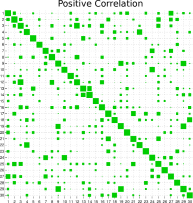
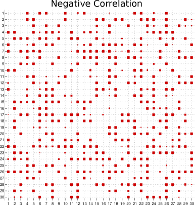
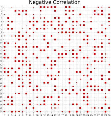
Figure 1 illustrates the DILN posterior for 10,000 articles from Wikipedia. The corpus is described by a set of topics—each topic is a distribution over words and is visualized by listing the most probable words—and the topics exhibit a correlation structure. For example, topic 3 (“party, election, vote”) is correlated with topic 12 (“constitution, parliament, council”) and topic 25 (“coup, army, military”). It is negatively correlated with topic 20 (“food, meat, drink”).

In DILN, each component is associated with a parameter (e.g., a topical distribution over terms) and a location in a latent space. For group-level distributions (e.g., document-specific distributions over topics), the correlation between component weights is determined by a kernel function of latent locations of these components. Since the correlation between occurrences is a posterior correlation, i.e., one that emerges from the data, the locations of the components are also latent. For example, we do not enforce a priori what the topics are and how they are correlated—this structure comes from the posterior analysis of the text.

We formulate two equivalent representations of DILN. We first formulate it as an HDP scaled by a Gaussian process (Rasmussen and Williams, 2006). This gives an intuitive picture of how the correlation between component weights enters the distribution and makes clear the relationship between DILN and the HDP. We then formulate DILN as a member of the normalized gamma family of random probability distributions. This lets us characterize the a priori correlation structure of the component proportions.

The central computational problem for DILN is approximate posterior inference. Given a corpus, we want to compute the posterior distribution of the topics, per-document topic proportions, and the latent locations of the topics. Using normalized the gamma construction of a random measure, we derive a variational inference algorithm (Jordan et al., 1999) to approximate the full posterior of a DILN mixed-membership model. (Moreover, this variational algorithm can be modified into a new posterior inference algorithm for HDP mixed-membership models.) We use variational inference to analyze several collections of documents, each on the order of thousands of articles, determining the number of topics based on the data and identifying an explicit correlation structure among the discovered topics. On four corpora (collected from Wikipedia, Science, The New York Times, and The Huffington Post), we demonstrate that DILN provides a better predictive model and an effective new method for summarizing and exploring text data. (Again, see Figure 1 and also Figures 4, 5 and 6.)

Variational inference turns the problem of approximating the posterior into an optimization problem. Recent research has used stochastic optimization to scale variational inference up to very large data sets (Hoffman, Blei and Bach, 2010; Armagan and Dunson, 2011), including our own research on HDP mixed-membership models (Wang, Paisley and Blei, 2011). We used the same strategy here to develop a scalable inference algorithm for DILN. This further expands the scope of stochastic variational inference to models (like DILN) whose latent variables do not enjoy pair-wise conjugacy. Using stochastic inference, we analyzed 352,549 thousand articles from Nature magazine, a corpus which would be computationally expensive with our previous variational algorithm.

Related research.

The parametric model most closely related to DILN is the correlated topic model (CTM) (Blei and Lafferty, 2007). The CTM is a mixed-membership model that allows topic occurrences to exhibit correlation. The CTM replaces the Dirichlet prior over topic proportions, which assumes near independence of the components, with a logistic normal prior (Aitchison, 1982). Logistic normal vectors are generated by exponentiating a multivariate Gaussian vector and normalizing to form a probability vector. The covariance matrix of the multivariate Gaussian distribution provides a means for capturing correlation structure between topic probabilities. Our goal in developing DILN was to form a Bayesian nonparametric variant of this kind of model.

The natural nonparametric extension of the logistic normal is a normalized exponentiated Gaussian process (Lenk, 1988; Rasmussen and Williams, 2006). However, this cannot function as a prior for nonparametric correlated topic modeling. The key property of the HDP (and DILN) is that the same set of components are shared among the groups. This sharing arises because the group-level distributions on the infinite topic space are discrete probability measures over the same set of atoms. Using the model of Lenk (1988) in a hierarchical setting does not provide such distributions. The “infinite CTM” is therefore not a viable alternative to the HDP.

In the Bayesian nonparametric literature, another related line of work focuses on dependent probability distributions where the dependence is defined on predictors observed for each data point. MacEachern (1999) introduced dependent Dirichlet processes (DDPs), which allow data-dependent variation in the atoms of the mixture, and have been applied to spatial modeling (Gelfand, Kottas and MacEachern, 2005; Rao and Teh, 2009). Other dependent priors allow the mixing weights themselves to vary with predictors (Griffin and Steel, 2006; Duan, Guindani and Gelfand, 2007; Dunson and Park, 2008; Ren et al., 2011). Still other methods consider the weighting of multiple DP mixture models using spatial information (Muller, Quintana and Rosner, 2004; Dunson, Pillai and Park, 2007).

These methods all use the spatial dependence between observations to construct observation-specific probability distributions. Thus they condition on known locations (often geospatial) for the data. In contrast, the latent locations of each component in DILN do not directly interact with the data, but with each other. That is, the correlations induced by these latent locations influence the mixing weights for a data group prior to producing its observations in the generative process. Unlike DDP models, our observations are not equipped with locations and do not a priori influence component probabilities. The modeling ideas behind DILN and behind DDPs are separate, though it is possible to develop dependent DILN models, just as dependent HDP models have been developed (MacEachern, 1999).

This paper is organized as follows. In Section 2 we review the HDP and discuss its representation as a normalized gamma process. In Section 3 we present the discrete infinite logistic normal distribution, first as a scaling of an HDP with an exponentiated Gaussian process and then using a normalized gamma construction. In Section 4 we use this gamma construction to derive a mean-field variational inference algorithm for approximate posterior inference of DILN topic models, and we extend this algorithm to the stochastic variational inference setting. Finally, in Section 5 we provide an empirical study of the DILN topic model on five text corpora.

2 Background: The Hierarchical Dirichlet Process

The discrete infinite logistic normal (DILN) prior for mixed-membership models is an extension of the hierarchical Dirichlet process (HDP) (Teh et al., 2006). In this section, we review the HDP and reformulate it as a normalized gamma process.

2.1 The original formulation of the hierarchical Dirichlet process

The Dirichlet process (Ferguson, 1973) is useful as a Bayesian nonparametric prior for mixture models since it generates distributions on infinite parameter spaces that are almost surely discrete (Blackwell and MacQueen, 1973; Sethuraman, 1994). Given a space $\Omega$ with a corresponding Borel $\sigma$-algebra $\mathcal{B}$ and base measure $\alpha G_{0}$, where $\alpha>0$ and $G_{0}$ is a probability measure, Ferguson (1973) proved the existence of a process $G$ on $(\Omega,\mathcal{B})$ such that for all measurable partitions $\{B_{1},\dots,B_{K}\}$ of $\Omega$,

$$(G(B_{1}),\dots,G(B_{K}))\sim\mathrm{Dirichlet}(\alpha G_{0}(B_{1}),\dots,\alpha G_{0}(B_{K})).$$ (1)

This is called a Dirichlet process and is denoted $G\sim\textrm{DP}(\alpha G_{0})$. Sethuraman (1994) gave a proof of the almost sure (a.s.) discreteness of $G$ by way of a stick-breaking representation (Ishwaran and James, 2001); we will review this stick-breaking construction later. Blackwell and MacQueen (1973) gave an earlier proof of this discreteness using Pólya urn schemes. The discreteness of $G$ allows us to write it as

$$G=\sum_{k=1}^{\infty}p_{k}\delta_{\eta_{k}},$$

where each atom $\eta_{k}$ is generated i.i.d. from the base distribution $G_{0}$, and the atoms are given random probabilities $p_{k}$ whose distribution depends on a scaling parameter $\alpha>0$ such that smaller values of $\alpha$ lead to distributions that place more mass on fewer atoms. The DP is most commonly used as a prior for a mixture model, where $G_{0}$ is a distribution on a model parameter, $G\sim\textrm{DP}(\alpha G_{0})$ and each data point is drawn from a distribution family indexed by a parameter drawn from $G$ (Ferguson, 1983; Lo, 1984).

When the base measure $G_{0}$ is non-atomic, multiple draws from the DP prior place their probability mass on an a.s. disjoint set of atoms. That is, for $G_{1},G_{2}\stackrel{{\scriptstyle iid}}{{\sim}}\textrm{DP}(\alpha G_{0})$, an atom $\eta_{k}$ in $G_{1}$ will a.s. not appear in $G_{2}$, i.e., $G_{1}(\{\eta_{k}\})>0\implies G_{2}(\{\eta_{k}\})=0$ a.s. The goal of mixed-membership modeling is to use all groups of data to learn a shared set of atoms. The hierarchical Dirichlet process (Teh et al., 2006) was introduced to allow multiple Dirichlet processes to share the same atoms. The HDP is a prior for a collection of random distributions $(G_{1},\dots,G_{M})$. Each $G_{m}$ is i.i.d. DP distributed with a base probability measure that is also a Dirichlet process,

$$G\sim\mathrm{DP}(\alpha G_{0}),\quad\quad G_{m}\,|\,G~{}\stackrel{{\scriptstyle iid}}{{\sim}}~{}\mathrm{DP}(\beta G).$$ (2)

The hierarchical structure of the HDP ensures that each $G_{m}$ has probability mass distributed across a shared set of atoms, which results from the a.s. discreteness of the second-level base measure $\beta G$. Therefore, the same subset of atoms will be used by all groups of data, but with different probability distributions on these atoms for each group.

Where the DP allows us to define a mixture model, the HDP allows us to define a mixed-membership model. Given an HDP $(G_{1},\dots,G_{M})$, each $G_{m}$ generates its associated group of data from a mixture model,

$$X_{n}^{(m)}\,|\,\theta_{n}^{(m)} \stackrel{{\scriptstyle ind}}{{\sim}} f(X|\theta_{n}^{(m)}),\quad n=1,\dots,N_{m},$$ (3)

$$\theta_{n}^{(m)}\,|\,G_{m} \stackrel{{\scriptstyle iid}}{{\sim}} G_{m},\quad\quad\quad\quad n=1,\dots,N_{m}.$$ (4)

The datum $X_{n}^{(m)}$ denotes the $n$th observation in the $m$th group and $\theta_{n}^{(m)}$ denotes its associated parameter drawn from the mixing distribution $G_{m}$, with $\mathrm{Pr}(\theta_{n}^{(m)}=\eta_{k}|G_{m})=G_{m}(\{\eta_{k}\})$. The HDP can be defined to an arbitrary depth, but we focus on the two-level process described above.

When used to model documents, the HDP is a prior for topic models. The observation $X_{n}^{(m)}$ is the $n$th word in the $m$th document and is drawn from a discrete distribution on words in a vocabulary, $X_{n}^{(m)}|\theta_{n}^{(m)}\sim\mathrm{Discrete}(\theta_{n}^{(m)})$, where $\theta_{n}^{(m)}$ is the $V$-dimensional word probability vector selected according to $G_{m}$ by its corresponding word. The base probability measure $G_{0}$ is usually a symmetric Dirichlet distribution on the vocabulary simplex. Given a document collection, posterior inference yields a set of shared topics and per-document proportions over all topics. Unlike its finite counterpart, latent Dirichlet allocation (Blei, Ng and Jordan, 2003), the HDP topic model determines the number of topics from the data (Teh et al., 2006).

2.2 The HDP as a normalized gamma process

The DP has several representations, including a gamma process representation (Ferguson, 1973) and a stick-breaking representation (Sethuraman, 1994). In constructing HDPs, we will take advantage of each of these representations at different levels of the hierarchy.

We construct the top-level DP using stick-breaking (Sethuraman, 1994),

$$G=\sum_{k=1}^{\infty}V_{k}\prod_{j=1}^{k-1}(1-V_{j})\delta_{\eta_{k}},\quad V_{k}\stackrel{{\scriptstyle iid}}{{\sim}}\mathrm{Beta}(1,\alpha),\quad\eta_{k}\stackrel{{\scriptstyle iid}}{{\sim}}G_{0}.$$ (5)

The name comes from an interpretation of $V_{k}$ as the proportion broken from the remainder of a unit-length stick $\prod_{j=1}^{k-1}(1-V_{j})$. The resulting absolute length of this stick forms the probability of atom $\eta_{k}$. Letting $p_{k}:=V_{k}\prod_{j=1}^{k-1}(1-V_{j})$, this method of generating DPs produces probability measures that are size-biased according to index $k$ since $\mathbb{E}[p_{k}]>\mathbb{E}[p_{j}]$ for $k<j$.

Turning to the second-level DP $G_{m}$, we now use a normalized gamma process. Recall that a $K$-dimensional Dirichlet-distributed vector $(Y_{1},\dots,Y_{K})\sim\mathrm{Dirichlet}(c_{1},\dots,c_{K})$ with $c_{i}>0$ and $\sum_{j}c_{j}<\infty$ can be generated for any value of $K$ by drawing $Z_{i}\stackrel{{\scriptstyle ind}}{{\sim}}\mathrm{Gamma}(c_{i},1)$ and defining $Y_{i}:=Z_{i}/\sum_{j}Z_{j}$ (Ishwaran and Zarepour, 2002). Ferguson (1973) focused on the infinite extension of this representation as a normalized gamma process. Since $p_{k}>0$ for all atoms $\eta_{k}$ in $G$, and also because $\sum_{j=1}^{\infty}\beta p_{j}=\beta<\infty$, we can construct each $G_{m}$ using the following normalization of a gamma process,

$$G_{m}\,|\,G,Z=\sum_{k=1}^{\infty}\frac{Z_{k}^{(m)}}{\sum_{j=1}^{\infty}Z_{j}^{(m)}}\delta_{\eta_{k}},\quad Z_{k}^{(m)}\,|\,G\stackrel{{\scriptstyle ind}}{{\sim}}\mathrm{Gamma}(\beta p_{k},1).$$ (6)

The gamma process representation of the DP is discussed by Ferguson (1973), Kingman (1993) and Ishwaran and Zarepour (2002), but it has not been applied to the HDP. In DILN we will mirror this type of construction of the HDP—a stick-breaking construction for the top-level DP and a gamma process construction for the second-level DPs. This will let us better articulate model properties and also make inference easier.

3 The Discrete Infinite Logistic Normal Distribution

The HDP prior has the hidden assumption that the presence of one atom in a group is not a priori correlated with the presence of another atom (aside from the negative correlation imposed by the probability simplex). At the group level the HDP cannot model correlation structure between the components’ probability mass. To see this, note that the gamma process used to construct each group-level distribution is an example of a completely random measure (Kingman, 1993). That is, the unnormalized masses $(Z_{1}^{(m)},Z_{2}^{(m)},\dots)$ of the atoms $(\eta_{1},\eta_{2},\dots)$ of $G_{m}$ are independently drawn, and for all partitions $\{B_{1},\dots,B_{K}\}$ of $\Omega$ and given $S_{m}:=\sum_{j}Z_{j}^{(m)}$, the scaled random variables $S_{m}G_{m}(B_{1}),\dots,S_{m}G_{m}(B_{K})$ are independent. Thus, no correlation between per-group probabilities can be built into the HDP.

We introduced the discrete infinite logistic normal (DILN) as a modification of the HDP that can express such correlations (Paisley, Wang and Blei, 2011). The idea is that each atom lives in a latent location, and the correlation between atom probabilities is determined by their relative locations in the latent space. When analyzing data, modeling these correlations can improve the predictive distribution and provide more information about the underlying latent structure. DILN has two equivalent representations; we first describe it as a scaled HDP, with scaling determined by an exponentiated Gaussian process (Rasmussen and Williams, 2006). We then show how DILN fits naturally within the family of normalized gamma constructions of discrete probability distributions in a way similar to the discussion in Section 2.2 for the HDP.

3.1 DILN as a scaled HDP

DILN shares the same hierarchical structure described in Section 2.2 for the HDP—there is an infinite set of components and each group exhibits those components with different probabilities. In DILN, we further associate each component with a latent location in $\mathbb{R}^{d}$. (The dimension $d$ is predefined.) The model then uses these locations to influence the correlations between the probabilities of the components for each group-level distribution. In posterior inference, we infer both the components and their latent locations. Thus, through the inferred locations, we can estimate the correlation structure among the components.

Let $G_{0}$ be a base distribution over parameter values $\eta\in\Omega$, and let $L_{0}$ be a non-atomic base distribution over locations, $\ell\in\mathbb{R}^{d}$. We first draw a top-level Dirichlet process with a product base measure $\alpha G_{0}\times L_{0}$,

$$G\sim\textrm{DP}(\alpha G_{0}\times L_{0}).$$ (7)

Here, $G$ is a probability measure on the space $\Omega\times\mathbb{R}^{d}$. For each atom $\{\eta,\ell\}\in\Omega\times\mathbb{R}^{d}$, we think of $\eta\in\Omega$ as living in the parameter space, and $\ell\in\mathbb{R}^{d}$ as living in the location space.

In the second level of the process, the model uses both the probability measure $G$ and the locations of the atoms to construct group-level probability distributions. This occurs in two steps. In the first step, we independently draw a Dirichlet process and a Gaussian process using the measure and atoms of $G$,

$$G_{m}^{\textrm{DP}}\,|\,G\sim\textrm{DP}(\beta G),\quad W_{m}(\ell)\sim\textrm{GP}(\boldsymbol{\mu}(\ell),\boldsymbol{\mathrm{K}}(\ell,\ell^{\prime})).$$ (8)

The Dirichlet process $G_{m}^{\textrm{DP}}$ provides a new, initial distribution on the atoms of $G$ for group $m$. The Gaussian process $W_{m}$ is defined on the locations of the atoms of $G$ and results in a random function that can be evaluated using the location of each atom. The covariance between $W_{m}(\ell)$ and $W_{m}(\ell^{\prime})$ is determined by a kernel function $\boldsymbol{\mathrm{K}}(\ell,\ell^{\prime})$ on their respective locations.

The second step is to form each group-level distribution by scaling the probabilities of each second-level Dirichlet process by the exponentiated values of its corresponding Gaussian process,

$$G_{m}(\{\eta,\ell\})\,|\,G_{m}^{\textrm{DP}},W_{m}\propto G_{m}^{\textrm{DP}}(\{\eta,\ell\})\exp\{W_{m}(\ell)\}.$$ (9)

Since we define $G_{0}$ and $L_{0}$ to be non-atomic, all $\eta$ and $\ell$ in $G$ are a.s. distinct, and evaluating the Gaussian process $W_{m}$ at a location $\ell$ determines its atom $\{\eta,\ell\}$. We satisfy two objectives with this representation: ($i$) the probability measure $G_{m}$ is discrete, owing to the discreteness of $G_{m}^{\textrm{DP}}$, and ($ii$) the probabilities in $G_{m}$ are explicitly correlated, due to the exponentiated Gaussian process. We emphasize that these correlations arise from latent locations and in posterior inference we infer these locations from data.

Figure 2: A graphical model of the normalized gamma construction of the DILN topic model.

3.2 A normalized gamma construction of DILN

We now turn to a normalized gamma construction of DILN. We show that the DILN prior uses the second parameter of the gamma distribution in the normalized gamma construction of the HDP to model the covariance structure among the components of $G_{m}$. This representation facilitates approximate posterior inference described in Section 4, and helps clarify the covariance properties of the group-level distributions over atoms.

We use a stick-breaking construction of the top-level Dirichlet process (Equation 7),

$$G=\sum_{k=1}^{\infty}V_{k}\prod_{j=1}^{k-1}(1-V_{j})\delta_{\{\eta_{k},\ell_{k}\}},\quad V_{k}\stackrel{{\scriptstyle iid}}{{\sim}}\mathrm{Beta}(1,\alpha),\quad\eta_{k}\stackrel{{\scriptstyle iid}}{{\sim}}G_{0},\quad\ell_{k}\stackrel{{\scriptstyle iid}}{{\sim}}L_{0}.$$ (10)

This is nearly the same as the top-level construction of the HDP given in Equation (5). The difference is that the product base measure is defined over the latent location $\ell_{k}$ as well as the component $\eta_{k}$ to form the atom $\{\eta_{k},\ell_{k}\}$.

We pattern the group-level distributions after the gamma process construction of the second-level DP in the HDP,

$$G_{m}\,|\,G,Z=\sum_{k=1}^{\infty}\frac{Z_{k}^{(m)}}{\sum_{j=1}^{\infty}Z_{j}^{(m)}}\delta_{\{\eta_{k},\ell_{k}\}},$$ (11)

$$\quad Z_{k}^{(m)}\,|\,G,W_{m}\sim\mathrm{Gamma}(\beta p_{k},\exp\{-W_{m}(\ell_{k})\}),\quad W_{m}\,|\,G\stackrel{{\scriptstyle iid}}{{\sim}}\mathrm{GP}(\boldsymbol{\mu}(\ell),\boldsymbol{\mathrm{K}}(\ell,\ell^{\prime})),$$

with $p_{k}:=V_{k}\prod_{j=1}^{k-1}(1-V_{j})$. Here, DILN differs from the HDP in that it uses the second parameter of the gamma distribution. In the appendix, we give a proof that the normalizing constant is almost surely finite.

We note that the locations $\ell_{k}$ contained in each atom no longer serve a function in the model after $G_{m}$ is constructed, but we include them in Equation (11) to be technically correct. The purpose of the locations $\{\ell_{k}\}$ is to generate sequences $Z_{1}^{(m)},Z_{2}^{(m)},\dots$ that are correlated, which is not achieved by the HDP. After constructing the weights of $G_{m}$, the locations have fulfilled their role and are no longer used downstream by the model.

We derive Equation (11) using a basic property of gamma distributed random variables. Recall that the gamma density is $f(z|a,b)=b^{a}z^{a-1}\exp\{-bz\}/\Gamma(a)$. Consider a random variable $y\sim\mathrm{Gamma}(a,1)$ that is scaled by $b>0$ to produce $z=by$. Then $z\sim\mathrm{Gamma}(a,b^{-1})$. In Equation (9) we scale atom $\{\eta,\ell\}$ of the Dirichlet process $G_{m}^{\textrm{DP}}$ by $\exp\{W_{m}(\ell)\}$. Using the gamma process representation of $G_{m}^{\textrm{DP}}$ given in Equation (6) and the countably infinite $G$ in Equation (10), we have that $G_{m}(\{\eta_{k},\ell_{k}\})\propto Y_{k}^{(m)}\exp\{W_{m}(\ell)\}$, where $Y_{k}^{(m)}\sim\mathrm{Gamma}(\beta p_{k},1)$. Since $Z_{k}^{(m)}:=Y_{k}^{(m)}\exp\{W_{m}(\ell)\}$ is distributed as $\mathrm{Gamma}(\beta p_{k},\exp\{-W_{m}(\ell_{k})\})$ by the above property of scaled gamma random variables, the construction in Equation (11) follows.

For the topic model, drawing an observation proceeds as for the HDP. We use a latent indicator variable $C_{n}^{(m)}$, which selects the index of the atom used by observation $X_{n}^{(m)}$. This indicator variable gives a useful hidden-data representation of the process for inference in mixture models (Escobar and West, 1995),

$$X_{n}^{(m)}\,|\,G_{m},C_{n}^{(m)}\stackrel{{\scriptstyle ind}}{{\sim}}\mathrm{Discrete}(\eta_{C_{n}^{(m)}}),\quad C_{n}^{(m)}\,|\,G_{m}\stackrel{{\scriptstyle iid}}{{\sim}}\sum_{k=1}^{\infty}\frac{Z_{k}^{(m)}}{\sum_{j=1}^{\infty}Z_{j}^{(m)}}\delta_{k}\,,$$ (12)

where the discrete distribution is on word index values $\{1,\dots,V\}$. We note that this discrete distribution is one of many possible data generating distributions, and changing this distribution and $G_{0}$ will allow for DILN to be used in a variety of other mixed-membership modeling applications (Erosheva, Fienberg and Joutard, 2007; Airoldi et al., 2008; Pritchard, Stephens and Donnelly, 2000). Figure 2 shows the graphical model of the DILN topic model.

3.3 The covariance structure of DILN

The two-parameter gamma representation of DILN permits simple calculation of the expectation, variance and covariance prior to normalization. We first give these values conditioning on the top-level Dirichlet process $G$ and integrating out the Gaussian process $W_{m}$. In the following calculations, we assume that the mean function of the Gaussian process is $\boldsymbol{\mu}(\cdot)=0$ and we define $k_{ij}:=\boldsymbol{\mathrm{K}}(\ell_{i},\ell_{j})$. The expectation, variance and covariance of $Z_{i}^{(m)}$ and $Z_{j}^{(m)}$ are

$$\mathbb{E}\left[Z^{(m)}_{i}|\beta,\boldsymbol{p},\boldsymbol{\mathrm{K}}\right] = \beta p_{i}\mathrm{e}^{\frac{1}{2}k_{ii}},$$ (13)

$$\mathbb{V}\left[Z^{(m)}_{i}|\beta,\boldsymbol{p},\boldsymbol{\mathrm{K}}\right] = \beta p_{i}\mathrm{e}^{2k_{ii}}+\beta^{2}p_{i}^{2}\mathrm{e}^{k_{ii}}\left(\mathrm{e}^{k_{ii}}-1\right),$$

$$\mathrm{Cov}\left[Z^{(m)}_{i},Z^{(m)}_{j}|\beta,\boldsymbol{p},\boldsymbol{\mathrm{K}}\right] = \beta^{2}p_{i}p_{j}\mathrm{e}^{\frac{1}{2}(k_{ii}+k_{jj})}\left(\mathrm{e}^{k_{ij}}-1\right).$$

Observe that the covariance is similar to the unnormalized logistic normal (Aitchison, 1982), but with the additional term $\beta^{2}p_{i}p_{j}$. In general, these $p_{i}$ terms show how sparsity is enforced by the top-level DP, since both the expectation and variance terms go to zero exponentially fast as $i$ increases.

These values can also be calculated with the top-level Dirichlet process integrated out using the tower property of conditional expectation. They are

$$\mathbb{E}\left[Z^{(m)}_{i}|\alpha,\beta,\boldsymbol{\mathrm{K}}\right] = \beta\mathbb{E}[p_{i}]\mathrm{e}^{\frac{1}{2}k_{ii}},$$ (14)

$$\mathbb{V}\left[Z^{(m)}_{i}|\alpha,\beta,\boldsymbol{\mathrm{K}}\right] = \beta\mathbb{E}[p_{i}]\mathrm{e}^{2k_{ii}}+\beta^{2}\mathbb{E}[p_{i}^{2}]\mathrm{e}^{2k_{ii}}-\beta^{2}\mathbb{E}[p_{i}]^{2}\mathrm{e}^{k_{ii}},$$

$$\mathrm{Cov}\left[Z^{(m)}_{i},Z^{(m)}_{j}|\alpha,\beta,\boldsymbol{\mathrm{K}}\right] = \beta^{2}\mathbb{E}[p_{i}p_{j}]\mathrm{e}^{\frac{1}{2}(k_{ii}+k_{jj})+k_{ij}}-\beta^{2}\mathbb{E}[p_{i}]\mathbb{E}[p_{j}]\mathrm{e}^{\frac{1}{2}(k_{ii}+k_{jj})}.$$

The values of the expectations in Equation (14) are

$$\mathbb{E}[p_{i}]=\frac{\alpha^{i-1}}{(1+\alpha)^{i}},\quad\mathbb{E}[p_{i}^{2}]=\frac{2\alpha^{i-1}}{(1+\alpha)(2+\alpha)^{i}},\quad\mathbb{E}[p_{i}p_{j}]=\frac{\alpha^{i-1}}{(2+\alpha)^{j}(1+\alpha)^{i-j+1}},~{}~{}i>j.$$

Note that some covariance remains when $k_{ij}=0$, since the conditional independence induced by $\boldsymbol{p}$ is no longer present. The available covariance structure depends on the kernel. For example, when a Gaussian kernel is used, a structured negative covariance is not achievable since $k_{ij}\geq 0$. We next discuss one possible kernel function, which we will use in our inference algorithm and experiments.

3.4 Learning the kernel for DILN

In our formulation of DILN, we have left the kernel function undefined. In principle, any kernel function can be used, but in practice some kernels yield simpler inference algorithms than others. For example, while a natural choice for $\boldsymbol{\mathrm{K}}(\ell,\ell^{\prime})$ is the Gaussian kernel, we found that the resulting variational inference algorithm was computationally expensive because it required many matrix inversions to infer the latent locations. In this section, we define an alternative kernel. In the next section, we will see that this leads to simple algorithms for approximate inference of the latent locations $\ell$.

We model the location of a component with a zero-mean Gaussian vector in $\mathbb{R}^{d}$. We then form the kernel by taking the dot product of these vectors. That is, for components $k$ and $j$, we draw locations and parameterize the Gaussian process for $W_{m}$ as

$$\ell_{k}\stackrel{{\scriptstyle iid}}{{\sim}}\mbox{Normal}(0,cI_{d}),\quad\quad\boldsymbol{\mu}(\ell_{k})=0,\quad\quad\boldsymbol{\mathrm{K}}(\ell_{k},\ell_{j})=\ell_{k}^{T}\ell_{j}.$$ (15)

With this specification, all $p$-dimensional ($p\leq d$) sub-matrices of $\boldsymbol{\mathrm{K}}$ are Wishart-distributed with parameters $p$ and $cI_{p}$ (Dawid, 1981). However, this kernel is problematic. When the number of components $p$ is greater than $d$, it will produce singular covariance matrices that cannot be inverted in the Gaussian likelihood function of $W_{m}$, an inversion that is required during inference. While in parametric models we might place constraints on the number of components, our prior is nonparametric. We have an infinite number of components and therefore $\boldsymbol{\mathrm{K}}$ must be singular.

We solve this problem by forming an equivalent representation of the kernel in Equation (15) that yields a more tractable joint likelihood function. This representation uses auxiliary variables as follows. Let $u\sim\mathrm{Normal}(0,I_{d})$ and recall that for a vector $z=B^{T}u$, the marginal distribution of $z$ is $z|B\sim\mathrm{Normal}(0,B^{T}B)$. In our case, $B^{T}B$ is the inner product kernel and the columns of $B$ correspond to component locations, $B=[\ell_{1},\ell_{2},\cdots]$.

With this in mind, we use the following construction of the Gaussian process $W_{m}$,

$$\quad W_{m}(\ell_{k})=\ell^{T}_{k}u_{m},\quad\quad u_{m}\sim\mathrm{Normal}(0,I_{d}).$$ (16)

Marginalizing the auxiliary vector $u_{m}$ gives the desired $W_{m}(\ell_{k})\sim\mathrm{GP}(0,\boldsymbol{\mathrm{K}}(\ell_{k},\ell_{j}))$.

The auxiliary vector $u_{m}$ allows for tractable inference of Gaussian processes that lie in a low-dimensional subspace. Aside from analytical tractability, the vector $u_{m}$ can be interpreted as a location for group $m$. (This is not to be confused with the location of component $k$, $\ell_{k}$.) The group locations let us measure similarity between groups, such as document similarity in the topic modeling case. In the following sections, we no longer work directly with $W_{m}(\ell_{k})$, but rather the dot product $\ell_{k}^{T}u_{m}$ through inference of $\ell$ and $u$.

4 Variational Inference for DILN

In Bayesian nonparametric mixed-membership modeling, the central computational problem is posterior inference. However, computing the exact posterior is intractable. For HDP-based models, researchers have developed several approximate methods (Teh et al., 2006; Liang et al., 2007; Teh, Kurihara and Welling, 2009; Wang, Paisley and Blei, 2011).

In this paper, we derive a mean-field variational inference algorithm (Jordan et al., 1999; Wainwright and Jordan, 2008) to approximate the posterior of a DILN mixed-membership model. We focus on topic modeling but note that our algorithm can be applied (with a little modification) to any DILN mixed-membership model. In addition, since the HDP is an instance of DILN, this algorithm also provides an inference method for HDP mixed-membership models.

Variational methods for approximate posterior inference attempt to minimize the Kullback-Leibler divergence between a factorized distribution over the hidden variables and the true posterior. The hidden variables in the DILN topic model can be broken into document-level variables (those defined for each document), and corpus-level variables (those defined across documents); the document-level variables are the unnormalized weights $Z_{k}^{(m)}$, topic indexes $C_{n}^{(m)}$, and document locations $u_{m}$; the corpus-level variables are the topic distributions $\eta_{k}$, proportions $V_{k}$, concentration parameters $\alpha$ and $\beta$, and topic locations $\ell_{k}$. Under the mean-field assumption the variational distribution that approximates the full posterior is factorized,

$$Q:=q(\alpha)q(\beta)\prod_{k=1}^{T}q(\eta_{k})q(V_{k})q(\ell_{k})\textstyle\prod_{m=1}^{M}q(Z_{k}^{(m)})q(C_{n}^{(m)})q(u_{m}).$$ (17)

We select the following variational distributions for each latent variable,

$$q(C_{n}^{(m)}) = \mathrm{Multinomial}(C_{n}^{(m)}|\phi_{n}^{(m)})$$

$$q(Z_{k}^{(m)}) = \mathrm{Gamma}(Z_{k}^{(m)}|a_{k}^{(m)},b_{k}^{(m)})$$

$$q(\eta_{k}) = \mathrm{Dirichlet}(\eta_{k}|\gamma_{k,1},\dots,\gamma_{k,D})$$

$$q(\ell_{k})q(u_{m}) = \delta_{\hat{\ell}_{k}}\cdot\delta_{\hat{u}_{m}}$$

$$q(V_{k}) = \delta_{\hat{V}_{k}}$$

$$q(\alpha)q(\beta) = \delta_{\hat{\alpha}}\cdot\delta_{\hat{\beta}}\,.$$ (18)

The set of parameters to these distributions are the variational parameters, represented by ${\mathrm{\Psi}}$. The goal of variational inference is to optimized these parameters to make the distribution $Q$ close in KL divergence to the true posterior. Minimizing this divergence is equivalent to maximizing a lower bound on the log marginal likelihood obtained from Jensen’s inequality,

$$\ln\int p({\mathrm{X}},{\mathrm{\Theta}})\,d{\mathrm{\Theta}}\geq\int Q({\mathrm{\Psi}})\ln\frac{p({\mathrm{X}},{\mathrm{\Theta}})}{Q({\mathrm{\Psi}})}\,d{\mathrm{\Theta}},$$ (19)

where ${\mathrm{\Theta}}$ stands for all hidden random variables. This objective has the form

$$\mathcal{L}({\mathrm{X}},{\mathrm{\Psi}})=\mathbb{E}_{Q}[\ln p({\mathrm{X}},{\mathrm{\Theta}})]+\mathbb{H}[Q].$$ (20)

We will find a locally optimal solution of this function using coordinate ascent, as detailed in the next section.

Note that we truncate the number of components at $T$ in the top-level Dirichlet process (Blei and Jordan, 2005). Kurihara, Welling and Vlassis (2006) show how infinite-dimensional objective functions can be defined for variational inference, but the conditions for this are not met by DILN. The truncation level $T$ should be set larger than the total number of topics expected to be used by the data. A value of $T$ that is set too small is easy to diagnose: the approximate posterior will use all $T$ topics. Setting $T$ large enough, the variational approximation will prefer a corpus-wide distribution on topics that is sparse. We contrast this with the CTM and other finite topic models, which fit a pre-specified number of topics to the data and potentially overfit if that number is too large.

We have selected several delta functions as variational distributions. In the case of the top-level stick-breaking proportions $V_{k}$ and second-level concentration parameter $\beta$, we have followed Liang et al. (2007) in doing this for tractability. In the case of the top-level concentration parameter $\alpha$, and topic and document locations $\ell_{k}$ and $u_{m}$, these choices simplify the algorithm.

Algorithm 1 Batch variational Bayes for DILN

Batch optimization of the variational lower bound $\mathcal{L}$
Optimize corpus-wide and document-specific variational parameters ${\mathrm{\Psi}}^{\prime}$ and ${\mathrm{\Psi}}_{m}$

1:  while ${\mathrm{\Psi}}^{\prime}$ and ${\mathrm{\Psi}}_{m}$ have not converged do

2:     for $m=1,\dots,M$ do

3:        Optimize ${\mathrm{\Psi}}_{m}$ (Equations 22–24)

4:     end for

5:     Optimize ${\mathrm{\Psi}}^{\prime}$ (Equations 25–29)

6:  end while

4.1 Coordinate ascent variational inference

We now present the variational inference algorithm for the DILN topic model. We optimize the variational parameters ${\mathrm{\Psi}}$ with respect to the variational objective function of Equation (20). For DILN, the variational objective expands to

$$\mathcal{L} = \sum_{m=1}^{M}\sum_{n=1}^{N_{m}}\sum_{k=1}^{T}\phi_{n,k}^{(m)}\mathbb{E}_{q}[\ln p(X_{n}^{(m)}|\eta_{k})]+\sum_{m=1}^{M}\sum_{n=1}^{N_{m}}\sum_{k=1}^{T}\phi_{n,k}^{(m)}\mathbb{E}_{q}[\ln p(C_{n}^{(m)}=k|Z_{1:T}^{(m)})]$$ (21)

$$+ \sum_{m=1}^{M}\sum_{k=1}^{T}\mathbb{E}_{q}[\ln p(Z_{k}^{(m)}|\beta p_{k},\ell_{k},u_{m})]+\sum_{k=1}^{T}\mathbb{E}_{q}[\ln p(\eta_{k}|\gamma)]+\sum_{k=1}^{T}\mathbb{E}_{q}[\ln p(V_{k}|\alpha)]$$

$$+ \sum_{k=1}^{T}\mathbb{E}_{q}[\ln p(\ell_{k})]+\sum_{m=1}^{M}\mathbb{E}_{q}[\ln p(u_{m})]+\mathbb{E}_{q}[\ln p(\alpha)]+\mathbb{E}_{q}[\ln p(\beta)]-\mathbb{E}_{Q}[\ln Q].$$

We use coordinate ascent to optimize this function, iterating between two steps. In the first step we optimize the document-level parameters for each document; in the second step we optimize the corpus-level parameters. Algorithm 1 summarizes this general inference structure.

Document-level parameters

For each document, we iterate between updating the variational distribution of per-word topic indicators $C_{n}^{(m)}$, unnormalized weights $Z_{k}^{(m)}$, and document locations $\hat{u}_{m}$.

Coordinate update of $q(C_{n}^{(m)})$

The variational distribution on the topic index for word $X_{n}^{(m)}$ is multinomial with parameter $\phi$. For $k=1,\dots,T$ topics

$$\phi_{n,k}^{(m)}\propto\exp\left\{\mathbb{E}_{Q}[\ln\eta_{k}(X_{n}^{(m)})]+\mathbb{E}_{Q}[\ln Z_{k}^{(m)}]\right\}.$$ (22)

Since $\phi_{n}^{(m)}=\phi_{n^{\prime}}^{(m)}$ when $X_{n}^{(m)}=X_{n^{\prime}}^{(m)}$, we only need to compute this update once for each unique word occurring in document $m$.

Coordinate update of $q(Z_{k}^{(m)})$

This variational gamma distribution has parameters $a_{k}^{(m)}$ and $b_{k}^{(m)}$. Let $N_{m}$ be the number of observations (e.g., words) in group $m$. After introducing an auxiliary parameter $\xi_{m}$ for each group-level distribution (discussed below), the updates are

$$a_{k}^{(m)} = \hat{\beta}p_{k}+\sum_{n=1}^{N_{m}}\phi_{n,k}^{(m)},$$

$$b_{k}^{(m)} = \exp\{-\hat{\ell}_{k}^{T}\hat{u}_{m}\}+\frac{N_{m}}{\xi_{m}}.$$ (23)

We again denote the top-level stick-breaking weights by $p_{k}=\hat{V}_{k}\prod_{j=1}^{k-1}(1-\hat{V}_{j})$. The expectations from this distribution that we use in subsequent updates are $\mathbb{E}_{Q}[Z_{k}^{(m)}]=a_{k}^{(m)}/b_{k}^{(m)}$ and $\mathbb{E}_{Q}[\ln Z_{k}^{(m)}]=\psi(a_{k}^{(m)})-\ln b_{k}^{(m)}$.

The auxiliary parameter allows us to approximate the term $\mathbb{E}_{Q}[\ln p(C_{n}^{(m)}=k|Z_{1:T}^{(m)})]$ appearing in the lower bound. To derive this, we use a first order Taylor expansion on the following intractable expectation,

$$-\mathbb{E}_{Q}\left[\ln\sum_{k=1}^{T}Z_{k}^{(m)}\right]\geq-\ln\xi_{m}-\frac{\sum_{k=1}^{T}\mathbb{E}_{Q}[Z_{k}^{(m)}]-\xi_{m}}{\xi_{m}}.$$

The update for the auxiliary variable $\xi_{m}$ is $\xi_{m}=\sum_{k=1}^{T}\mathbb{E}_{Q}[Z_{k}^{(m)}].$ See the appendix for the complete derivation.

Coordinate update of $q(u_{m})$

We update the location of the $m\mbox{th}$ document using gradient ascent, which takes the general form $\hat{u}_{m}^{\prime}=\hat{u}_{m}+\rho\nabla_{\hat{u}_{m}}\mathcal{L}$. We take several steps in updating this value within an iteration. For step $s$ we update $\hat{u}_{m}$ as

$$\hat{u}_{m}^{(s+1)}=(1-\rho_{s})\hat{u}_{m}^{(s)}+\rho_{s}\sum_{k=1}^{T}\left(\mathbb{E}_{Q}[Z_{k}]\mbox{e}^{-\hat{\ell}_{k}^{T}\hat{u}_{m}^{(s)}}-\hat{\beta}p_{k}\right)\hat{\ell}_{k}.$$ (24)

We let the step size $\rho$ be a function of step number $s$, and (for example) set it to $\rho_{s}=\frac{1}{T}(3+s)^{-1}$ for $s=1,\dots,20$. We use $1/T$ to give a per-topic average, which helps to stabilize the magnitude of the gradient by removing its dependence on truncation level $T$, while $(3+s)^{-1}$ shrinks the step size. For each iteration, we reset $s=1$.

Corpus-level parameters

After optimizing the variational parameters for each document, we turn to the corpus-level parameters. In the coordinate ascent algorithm, we update each corpus-level parameter once before returning to the document-level parameters.

Coordinate update of $q(\eta_{k})$

The variational distribution for the topic parameters is Dirichlet with parameter vector $\gamma_{k}$. For each of $d=1,\dots,D$ vocabulary words

$$\gamma_{k,d}=\gamma_{0}+\sum_{m=1}^{M}\sum_{n=1}^{N_{m}}\phi_{n,k}^{(m)}\mathbb{I}\left(X_{n}^{(m)}=d\right),$$ (25)

where $\gamma_{0}$ is the parameter for the base distribution $\eta_{k}\sim{\rm Dirichlet}(\gamma_{0})$. Statistics needed for this term can be updated in unison with updates to $q(C_{n}^{(m)})$ for faster inference.

Coordinate update of $q(V_{k})$

For $k=1,\dots,T-1$, the $q$ distribution for each $V_{k}$ is a delta function, $\delta_{\hat{V}_{k}}$. The truncation of the top-level DP results in $V_{T}:=1$. We use steepest ascent to jointly optimize $\hat{V}_{1},\dots,\hat{V}_{T-1}$. The gradient of each element is

$$\frac{\partial\mathcal{L}(\cdot)}{\partial\hat{V}_{k}}=-~{}\frac{\hat{\alpha}-1}{1-\hat{V}_{k}}+\hat{\beta}\left[\sum_{m}\left(\mathbb{E}_{Q}[\ln Z_{k}^{(m)}]-\hat{\ell}_{k}^{T}\hat{u}_{m}\right)-M\psi(\hat{\beta}p_{k})\right]\left[\frac{p_{k}}{\hat{V}_{k}}-\sum_{j>k}\frac{p_{j}}{1-\hat{V}_{k}}\right]$$ (26)

We observed similar performance using Newton’s method in our experiments.

Coordinate update of $q(\ell_{k})$

We update the location of the $k\mbox{th}$ topic by gradient ascent, which has the general form $\hat{\ell}_{k}^{\prime}=\hat{\ell}_{k}+\rho\nabla_{\hat{\ell}_{k}}\mathcal{L}$. We use the same updating approach as discussed for $\hat{u}_{m}$. For step $s$ within a given iteration, the update is

$$\hat{\ell}_{k}^{(s+1)}=(1-\rho_{s}/c)\hat{\ell}_{k}+\rho_{s}\sum_{m=1}^{M}\left(\mathbb{E}_{Q}[Z_{k}]\mbox{e}^{-\hat{u}_{m}^{T}\hat{\ell}_{k}^{(s)}}-\hat{\beta}p_{k}\right)\hat{u}_{m}.$$ (27)

As with $\hat{u}_{m}$, we let the step size $\rho$ be a function of step number $s$, and set it to $\rho_{s}=\frac{1}{M}(3+s)^{-1}$.

Coordinate updates of $q(\alpha)$ and $q(\beta)$

We place a $\mathrm{Gamma}(\tau_{1},\tau_{2})$ prior on $\alpha$ and model the posterior with a delta function. The update for this parameter is

$$\hat{\alpha}=\frac{K+\tau_{1}-2}{\tau_{2}-\sum_{k=1}^{K-1}\ln(1-\hat{V}_{k})}$$ (28)

In our empirical study we set $\tau_{1}=1$ and $\tau_{2}=10^{-3}$.

We also place a $\mathrm{Gamma}(\kappa_{1},\kappa_{2})$ prior on the second-level concentration parameter $\beta$ and optimize using gradient ascent. The first derivative is

$$\frac{\partial\mathcal{L}(\cdot)}{\partial\hat{\beta}}=\sum_{m,k}p_{k}\left(\psi(a_{k}^{(m)})-\ln b_{k}^{(m)}-\ell_{k}^{T}u_{m}-\psi(\hat{\beta}p_{k})\right)-\frac{\kappa_{1}-1}{\hat{\beta}}-\kappa_{2}.$$ (29)

We set $\kappa_{1}=1$ and $\kappa_{2}=10^{-3}$.

4.2 Stochastic variational inference

The algorithm of Section 4.1 can be called a batch algorithm because it updates all document-level parameters in one “batch” before updating the global parameters. A potential drawback of this batch inference approach for DILN (as well as potential Monte Carlo sampling algorithms) is that the per-iteration running time increases with an increasing number of groups. For many modeling applications, the algorithm may be impractical for large-scale problems.

One solution to the large-scale data problem is to sub-sample a manageable number of groups from the larger collection, and assume that this provides a good statistical representation of the entire data set. Indeed, this is the hope with batch inference, which views the data set as a representative sample from the larger, unseen population. However, in this scenario information contained in the available data set may be lost. Stochastic variational inference methods (Hoffman, Blei and Bach, 2010; Wang, Paisley and Blei, 2011; Sato, 2001) aim for the best of both worlds, allowing one to fit global parameters for massive collections of data in less time than it takes to solve problems of moderate size in the batch setting.

The idea behind stochastic variational inference is to perform stochastic optimization of the variational objective function in Equation (21). In topic modeling, we can construe this objective function as a sum over per-document terms and then obtain noisy estimates of the gradients by evaluating them on sets of documents sampled from the full corpus. By following these noisy estimates of the gradient with a decreasing step size, we are guaranteed convergence to a local optimum of the variational objective function (Robbins and Monro, 1951; Sato, 2001; Hoffman, Blei and Bach, 2010).

Algorithmically, this gives an advantage over the optimization algorithm of Section 4.1 for large-scale machine learning. The bottleneck of that algorithm is the variational “E step,” where the document-level variational parameters are optimized for all documents using the current settings of the corpus-level variational parameters (i.e., the topics and their locations, and $\alpha$, $\beta$). This computation may be wasteful, especially in the first several iterations, where the initial topics likely do not represent the corpus well. In contrast, the structure of a stochastic variational inference algorithm is to repeatedly subsample documents, analyze them, and then use them to update the corpus-level variational parameters. When the data set is massive, these corpus-level parameters can converge before seeing any document a second time.

In more detail, let ${\mathrm{X}}$ be a very large collection of $M$ documents. We separate the hidden variables ${\mathrm{\Theta}}$ into those for the top-level ${\mathrm{\Theta}}^{\prime}=\{\eta_{1:T},V_{1:T-1},\ell_{1:T},\alpha,\beta\}$ and the document-level ${\mathrm{\Theta}}_{m}=\{C^{(m)}_{1:N_{m}},u_{m},Z^{(m)}_{1:T}\}$ for $m=1,\dots,M$. These variables have variational parameters ${\mathrm{\Psi}}^{\prime}=\{\gamma_{1:T,1:D},\ell_{1:T},\hat{V}_{1:T-1},\hat{\alpha},\hat{\beta}\}$ and ${\mathrm{\Psi}}_{m}=\{\phi^{(m)}_{1:N_{m}},a^{(m)}_{1:T},b^{(b)}_{1:T},u_{m}\}$ for their respective $Q$ distributions. Because of the independence assumption between documents, the variational objective decomposes into a sum over documents,

$$\mathcal{L}({\mathrm{X}},{\mathrm{\Psi}})=\sum_{m=1}^{M}\mathbb{E}_{Q}[\ln p({\mathrm{X}}_{m},{\mathrm{\Theta}}_{m},{\mathrm{\Theta}}^{\prime})]+\sum_{m=1}^{M}\mathbb{H}[Q({\mathrm{\Theta}}_{m})]+\mathbb{H}[Q({\mathrm{\Theta}}^{\prime})].$$ (30)

As we discussed, in batch inference we optimize variational distributions on ${\mathrm{\Theta}}_{1},\dots,{\mathrm{\Theta}}_{M}$ before updating those on ${\mathrm{\Theta}}^{\prime}$. Now, consider an alternate objective function at iteration $t$ of inference,

$$\mathcal{L}^{(t)}({\mathrm{X}}_{m_{t}},{\mathrm{\Psi}}_{m_{t}},{\mathrm{\Psi}}^{\prime})=M\mathbb{E}_{Q}[\ln p({\mathrm{X}}_{m_{t}},{\mathrm{\Theta}}_{m_{t}}|{\mathrm{\Theta}}^{\prime})]+M\mathbb{H}[Q({\mathrm{\Theta}}_{m_{t}})]+\mathbb{E}_{Q}[\ln p({\mathrm{\Theta}}^{\prime})]+\mathbb{H}[Q({\mathrm{\Theta}}^{\prime})],$$ (31)

where $m_{t}$ is selected uniformly at random from $\{1,\dots,M\}$. An approach to optimize this objective function would be to first optimize the variational parameters of $Q({\mathrm{\Theta}}_{m_{t}})$, followed by a single gradient step for those of $Q({\mathrm{\Theta}}^{\prime})$. In determining the relationship between Equation (31) and Equation (30), note that under the uniform distribution $p(m_{t})$ on which document is selected,

$$\mathbb{E}_{p(m_{t})}[\mathcal{L}^{(t)}({\mathrm{X}}_{m_{t}},{\mathrm{\Psi}}_{m_{t}},{\mathrm{\Psi}}^{\prime})]=\mathcal{L}({\mathrm{X}},{\mathrm{\Psi}}).$$ (32)

We are thus stochastically optimizing $\mathcal{L}$. In practice, one document is not enough to ensure fast convergence of $Q({\mathrm{\Theta}}^{\prime})$. Rather, we select a subset $B_{t}\subset\{1,\dots,M\}$ at iteration $t$ and optimize

$$\mathcal{L}^{(t)}({\mathrm{X}}_{B_{t}},{\mathrm{\Psi}}_{B_{t}},{\mathrm{\Psi}}^{\prime}) = \frac{M}{|B_{t}|}\sum_{i\in B_{t}}\mathbb{E}_{Q}[\ln p({\mathrm{X}}_{i},{\mathrm{\Theta}}_{i}|{\mathrm{\Theta}}^{\prime})]+\frac{M}{|B_{t}|}\sum_{i\in B_{t}}\mathbb{H}[Q({\mathrm{\Theta}}_{i})]$$ (33)

$$+~{}\mathbb{E}_{Q}[\ln p({\mathrm{\Theta}}^{\prime})]~{}+~{}\mathbb{H}[Q({\mathrm{\Theta}}^{\prime})],$$

over the variational parameters of $Q({\mathrm{\Theta}}_{B_{t}})$. We again follow this with a step for the variational parameters of $Q({\mathrm{\Theta}}^{\prime})$, but this time using the information from documents indexed by $B_{t}$. That is, for some corpus-level parameter $\psi\in{\mathrm{\Psi}}^{\prime}$, the update of $\psi$ at iteration $t+1$ given $\psi$ at iteration $t$ is

$$\psi^{(t+1)}=\psi^{(t)}+\rho_{t}{\mathrm{A}}_{\psi}\nabla_{\psi}\mathcal{L}^{(t)}({\mathrm{X}}_{B_{t}},{\mathrm{\Psi}}_{B_{t}},{\mathrm{\Psi}}^{\prime}),$$ (34)

where ${\mathrm{A}}_{\psi}$ is a positive definite preconditioning matrix and $\rho_{t}>0$ is a step size satisfying

$$\sum_{t=1}^{\infty}\rho_{t}=\infty,\quad\quad\sum_{t=1}^{\infty}\rho_{t}^{2}<\infty.$$ (35)

In our experiments, we select the form $\rho_{t}=(\zeta+t)^{-\kappa}$ with $\kappa\in(0.5,1]$ and $\zeta>0$.

In some cases, the preconditioner ${\mathrm{A}}_{\psi}$ can be set to give simple and clear updates. For example, in the case of topic modeling, Hoffman, Blei and Bach (2010) show how the inverse Fisher information leads to very intuitive updates (see the next section). This is a special case of the theory outlined in Sato (2001) that arises in conjugate exponential family models. However, the Fisher information is not required for stochastic variational inference; we can precondition with the inverse negative Hessian or decide not to precondition.

Algorithm 2 Stochastic variational Bayes for DILN

Stochastically optimize the variational lower bound $\mathcal{L}$
Primary goal: Optimize corpus-wide variational parameters ${\mathrm{\Psi}}^{\prime}$
Secondary goal: Optimize document-specific parameters ${\mathrm{\Psi}}_{m}$ for $m=1,\dots,M$

1:  while ${\mathrm{\Psi}}^{\prime}$ has not converged do

2:     Select random subset $B_{t}\subset\{1,\dots,M\}$

3:     for $m\in B_{t}$ do

4:        Optimize ${\mathrm{\Psi}}_{m}$ (Equations 22–24)

5:     end for

6:     Set gradient step size $\rho_{t}=(\zeta+t)^{-\kappa}$, $\kappa\in(\frac{1}{2},1]$

7:     Update ${\mathrm{\Psi}}^{\prime}$ using gradient of $\mathcal{L}^{(t)}$ constructed from documents $m\in B_{t}$ (Equations 26, 27, 29, 34, 36–38)

8:  end while

9:  Optimize ${\mathrm{\Psi}}_{m}$ for $m=1,\dots,M$ using optimized ${\mathrm{\Psi}}^{\prime}$

4.2.1 The stochastic variational inference algorithm for DILN

The stochastic algorithm selects a subset of documents at step $t$, coded by a set of index values $B_{t}$, and optimizes the document-level parameters for these documents while holding all corpus-level parameters fixed. These parameters are the word indicators $C_{k}^{(m)}$, the unnormalized topic weights $Z_{k}^{(m)}$ and the document locations $u_{k}$. (See Section 4.1 for discussion on inference for these variables.) Given the values of the document-level variational parameters for documents indexed by $B_{t}$, we now describe the corpus-level updates in the stochastic inference algorithm. Algorithm 2 summarizes this general inference structure.

Stochastic update of $q(\eta_{k})$

This update follows from Hoffman, Blei and Bach (2010) and Wang, Paisley and Blei (2011). We set ${\mathrm{A}}_{\gamma_{k}}$ to be the inverse Fisher information of $q(\eta_{k})$,

$${\mathrm{A}}_{\gamma_{k}}=\left(-\frac{\partial^{2}\ln q(\eta_{k})}{\partial\gamma_{k}\partial\gamma_{k}^{T}}\right)^{-1}.$$

With this quantity, we take the product ${\mathrm{A}}_{\gamma_{k}}\nabla_{\gamma_{k}}\mathcal{L}^{(t)}({\mathrm{X}}_{B_{t}},{\mathrm{\Psi}}_{B_{t}},{\mathrm{\Psi}}^{\prime})$. This leads to give the following update for each $\gamma_{k,d}$,

$$\gamma_{k,d}^{(t+1)}=(1-\rho_{t})\gamma_{k,d}^{(t)}+\rho_{t}\left(\gamma_{0}+\frac{M}{|B_{t}|}\sum_{n,m\in B_{t}}\phi_{n,k}^{(m)}\mathbb{I}(X_{n}^{(m)}=d)\right).$$ (36)

In this case, premultiplying the gradient by the inverse Fisher information cancels the Fisher information in the gradient and thus removes the cross-dependencies between the components of $\gamma_{k}$. We use preconditioning to simplify the computation, rather than to speed up optimization. See Hoffman, Blei and Bach (2010), Wang, Paisley and Blei (2011) and Sato (2001) for details.

Stochastic update of $q(V_{k})$ and $q(\ell_{k})$

The stochastic updates of the delta $q$ distributions do not use the Fisher information. Rather, we update the vectors $V=[V_{1},\dots,V_{T-1}]^{T}$ and $\ell_{k}$ for $k=1,\dots,T$ by taking steps in their Newton directions using the data in batch $B_{t}$ to determine this direction. The gradients $\nabla\mathcal{L}$ for these parameters are given in the batch algorithm and their form is unchanged here. The key difference is that the gradient of these parameters at step $t$ is only calculated over documents with index values in $B_{t}$. We use the inverse negative Hessian as a preconditioning matrix for $\hat{\ell}_{k}$ and $(\hat{V}_{1},\dots,\hat{V}_{T-1})$. For $\ell_{k}$, the preconditioning matrix is

$${\mathrm{A}}_{\hat{\ell}_{k}}^{-1}=c^{-1}I+\sum_{m=1}^{M}(\mathbb{E}_{Q}[Z_{k}]\mbox{e}^{-\hat{\ell}_{k}\hat{u}_{m}})\hat{u}_{m}\hat{u}_{m}^{T}.$$ (37)

For $(\hat{V}_{1},\dots,\hat{V}_{T-1})$ the values of $({\mathrm{A}}_{\hat{V}}^{-1})_{kk}$ and $({\mathrm{A}}_{\hat{V}}^{-1})_{kr}$ are found from the second derivatives (with the second derivatives written for $r<k$)

$$-\frac{\partial^{2}\mathcal{L}(\cdot)}{\partial\hat{V}_{k}^{2}} = \frac{\hat{\alpha}-1}{(1-\hat{V}_{k})^{2}}+\hat{\beta}^{2}M\psi^{\prime}(\hat{\beta}p_{k})\frac{p_{k}}{\hat{V}_{k}}\left(\frac{p_{k}}{\hat{V}_{k}}-\sum_{j>k}\frac{p_{j}}{1-\hat{V}_{k}}\right),$$ (38)

$$-\frac{\partial^{2}\mathcal{L}(\cdot)}{\partial\hat{V}_{k}\partial\hat{V}_{r}} = -~{}\hat{\beta}^{2}M\psi^{\prime}(\hat{\beta}p_{k})\frac{p_{k}}{(1-\hat{V}_{r})}\left(\frac{p_{k}}{\hat{V}_{k}}-\sum_{j>k}\frac{p_{j}}{1-\hat{V}_{k}}\right)~{}+\hskip 90.3375pt$$ (39)

$$\hat{\beta}\left[\sum_{m}\left(\mathbb{E}_{Q}[\ln Z_{k}^{(m)}]-\hat{\ell}_{k}^{T}\hat{u}_{m}\right)-M\psi(\hat{\beta}p_{k})\right]\left[\frac{p_{k}}{\hat{V}_{k}(1-\hat{V}_{r})}-\sum_{j>k}\frac{p_{j}}{(1-\hat{V}_{k})(1-\hat{V}_{r})}\right].$$

Online update of $q(\alpha)$ and $q(\beta)$

The stochastic updates for $\hat{\beta}$ move in the direction of steepest ascent, calculated using the documents in the batch. Since this is a one-dimensional parameter, we optimize a batch-specific value for this parameter at step $t$, $\tilde{\beta}_{t}$, and set $\hat{\beta}_{t+1}=(1-\rho_{t})\hat{\beta}_{t}+\rho_{t}\tilde{\beta}_{t}$. The update for $\hat{\alpha}$ does not consider document-level parameters, and so this value follows the update given in Equation (28).

4.3 A new variational inference algorithm for the HDP

The variational inference algorithm above relates closely to one that can be derived for the HDP using the normalized gamma process representation of Section 2.2. The difference lies in the update for the topic weight $q(Z_{k}^{(m)})$ in Equation (4.1). In both algorithms, the update for its variational parameter $a_{k}^{(m)}$ contains the prior from the top-level DP, and the expected number of words in document $m$ drawn from topic $k$. The variational parameter $b^{(m)}$ distinguishes DILN from the HDP.

We can obtain a variational inference algorithm for the HDP by setting the first term in the update for $b_{k}^{(m)}$ equal to one. In contrast, the first term for DILN is $\exp\{-\hat{\ell}_{k}^{T}\hat{u}_{m}\}$, which is the Gaussian process that generates the covariance between component probability weights. Including or excluding this term switches between variational inference for DILN and variational inference for the HDP. See the appendix for a fuller derivation.

4.4 MCMC inference

Markov chain Monte Carlo (MCMC, Robert and Casella, 2004) sampling is a more common strategy for approximate posterior inference in Bayesian nonparametric models, and for the hierarchical Dirichlet process in particular. In MCMC methods, samples are drawn from a carefully designed Markov chain, whose stationary distribution is the target posterior of the model parameters. MCMC is convenient for the many Bayesian nonparametric models that are amenable to Gibbs sampling, where the Markov chain iteratively samples from the conditional distribution of each latent variable given all of the other latent variables and the observations.

However, Gibbs sampling is not an option for DILN because the Gaussian process component does not have a closed-form full conditional distribution. One possible sampling algorithm for DILN inference would use Metropolis-Hastings (Hastings, 1970), where samples are drawn from a proposal distribution and then accepted or rejected. Designing a good proposal distribution is the main problem in designing Metropolis-Hastings algorithms, and in DILN this problem is more difficult than usual because the hidden variables are highly correlated.

Recently, slice sampling has been applied to sampling of infinite mixture models by turning the problem into a finite sampling problem (Griffin and Walker, 2010; Kalli, Griffin and Walker, 2011). These methods apply when the mixture weights are either from a simple stick-breaking prior or a normalized random measures that can be simulated from a Poisson process. Neither of these settings applies to DILN because the second-level DP is a product of a DP and an exponentiated GP. Furthermore, it is not clear how to extend slice sampling methods to hierarchical models like the HDP or DILN.

Variational methods mitigate all these issues by using optimization to approximate the posterior. Our algorithm sacrifices the theoretical (and eventual) convergence to the full posterior in favor of a simpler distribution that is fit to minimize its KL-divergence to the posterior. Though we must address issues of local minima in the objective, we do not need to develop complicated proposal distributions or solve the difficult problem of assessing convergence of a high-dimensional Markov chain to its stationary distribution. Furthermore, variational inference is ideally suited to the stochastic optimization setting, allowing for approximate inference with very large data sets.

5 Empirical study

We evaluate the DILN topic model with both batch and stochastic inference. For batch inference, we compare with the HDP and correlated topic model (CTM) on four text corpora: The Huffington Post, The New York Times, Science and Wikipedia. We divide each corpus into five training and testing groups selected from a larger set of documents (see Table 1).

For stochastic inference, we use the Nature corpus to assess performance. This corpus contains 352,549 documents spanning 1869-2003; we used a vocabulary of 4,253 words. We compare stochastic DILN with a stochastic HDP algorithm and with online LDA (Hoffman, Blei and Bach, 2010).

Table 1: Data sets. Five training/testing sets were constructed by selecting the number of documents shown for each corpus from larger data sets.

Corpus	# training	# testing	vocabulary size	# total words
Huffington Post	3,000	1,000	6,313	660,000
New York Times	5,000	2,000	3,012	720,000
Science	5,000	2,000	4,403	1,380,000
Wikipedia	5,000	2,000	6,131	1,770,000

5.1 Evaluation metric

Before discussing the experimental setup and results, we discuss our method for evaluating performance. We evaluate the approximate posterior of all models by measuring its predictive ability on held-out documents. Following Asuncion et al. (2009), we randomly partition each test document into two halves and evaluate the conditional distribution of the second half given the first half and the training data. Operationally, we use the first half of each document to find estimates of document-specific topic proportions and then evaluate how well these combine with the fitted topics to predict the second half of the document.

More formally, denote the training data by ${\cal D}$, a test document as ${\mathrm{X}}$, which is divided into halves ${\mathrm{X}}^{\prime}$ and ${\mathrm{X}}^{\prime\prime}$. We want to calculate the conditional marginal probability,

$$p({{\mathrm{X}}}^{\prime\prime}|{{\mathrm{X}}}^{\prime},{\cal D})=\int_{\Omega_{\boldsymbol{\eta},\boldsymbol{Z}}}\prod_{n=1}^{N}\left\{\sum_{k=1}^{T}p({X}^{\prime\prime}_{n}|\eta_{k})p({C}^{\prime\prime}_{n}=k|{Z_{1:T}})\right\}dQ(\boldsymbol{Z})dQ(\boldsymbol{\eta})$$ (40)

where $N$ is the number of observations constituting ${\mathrm{X}}^{\prime\prime}$, $C_{n}^{\prime\prime}$ is the latent indicator associated with the $n$th word in ${\mathrm{X}}^{\prime\prime}$, and $\boldsymbol{\eta}:=\eta_{1:T}$ and $\boldsymbol{Z}:=Z_{1:T}$.

Since the integral in Equation (40) is intractable, we sample i.i.d. values from the factorized distributions $Q({Z_{1:T}})$ and $Q(\eta_{1:T})$ for approximation. We note that the information regarding the document’s correlation structure can be found in $Q({Z_{1:T}})$.

We then use this approximation of the marginal likelihood to compute the average per-word perplexity for the second half of the test document,

$${\rm perplexity}=\exp\left\{\frac{-\ln p({{\mathrm{X}}}^{\prime\prime}|{{\mathrm{X}}}^{\prime})}{N}\right\},$$ (41)

with lower perplexity indicating better performance. Note that the term $\ln p({{\mathrm{X}}}^{\prime\prime}|{{\mathrm{X}}}^{\prime})$ involves a sum over the $N$ words in ${\mathrm{X}}^{\prime\prime}$. Also note that this is an objective measure of the predictive performance of the predictive probability distribution computed from the variational approximation. It is a good measure of performance (of the model and the variational inference algorithm) because it does not rely on the closeness of the variational distribution to the true posterior, as measured by the variational lower bound. That closeness, much like whether a Markov chain has converged to its stationary distribution, is difficult to assess.

Figure 3: Perplexity results for four text corpora and averaged over five training/testing sets. For a fixed Dirichlet hyperparameter, the DILN topic model typically achieves better perplexity than both the HDP and CTM models. In all corpora, DILN achieves the best perplexity overall.

5.2 Experimental setup and results

Batch variational inference experiments

We trained all models using variational inference; for the CTM, this is the algorithm given in Blei and Lafferty (2007); for the HDP, we use the inference method from Section 4. For DILN, we use a latent space with $d=20$ and set the location variance parameter $c=1/20$. For DILN and the HDP, we truncate the top-level stick-breaking construction at $T=200$ components. For the CTM, we consider $K\in\{20,50,150\}$ topics. In our experiments, both DILN and HDP used significantly fewer topics than the truncation level, indicating that the truncation level was set high enough. The CTM is not sparse in this sense.

We initialize all models in the same way; to initialize the variational parameters of the topic Dirichlet, we first cluster the empirical word distributions of each document with three iterations of k-means using the $L_{1}$ distance measure. We then reorder these topics by their usage according to the indicators produced by k-means. We scale these k-means centroids and add a small constant plus noise to smooth the initialization. The other parameters are initialized to values that favor a uniform distribution on these topics. Variational inference is terminated when the fractional change in the lower bound of Equation (21) falls below $10^{-3}$. We run each algorithm using five different topic Dirichlet hyperparameter settings: $\gamma_{0}\in\{0.1,0.25,0.5,0.75,1.0\}$.

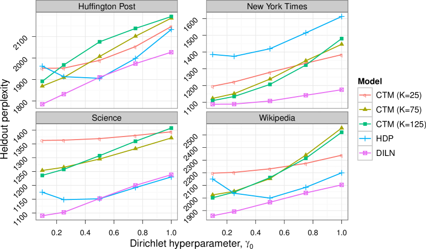
Figure 3 contains testing results for the four corpora. In general, DILN outperforms both the HDP and CTM. Given that the inference algorithms for DILN and the HDP are only different in the one term discussed in Section 4.3, this demonstrates that the latent location space models a correlation structure that helps in predicting words. Computation time for DILN and the HDP was comparable, both requiring on the order of one minute per iteration. Depending on the truncation level, the CTM was slightly to significantly faster than both DILN and the HDP.

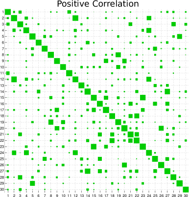
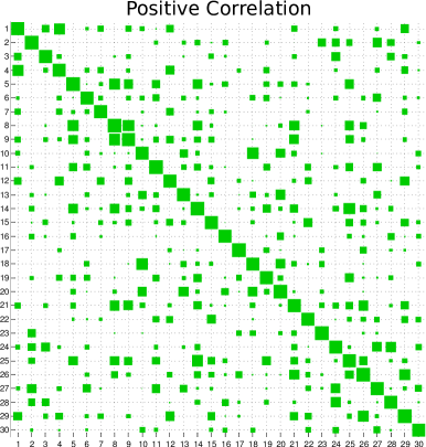
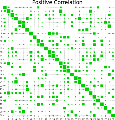
We display the learned correlation structure for the four corpora in Figures 4–6. (see Figure 1 for results on a slightly larger Wikipedia corpus.) In these figures, we represent the 30 most probable topics by their ten most probable words. Above these lists, we show the positive and negative correlations learned using the latent locations $\ell_{k}$. For two topics $i$ and $j$ this value is $\ell_{i}^{T}\ell_{j}/\|\ell_{i}\|_{2}\|\ell_{j}\|_{2}$. From these figures, we see that DILN learns meaningful underlying correlations in topic expression within a document.

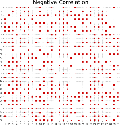Topic 1: campaign, democratic, candidate, republican, election, voter, political, presidential, vote, party

Topic 2: game, victory, second, score, third, win, team, play, season, lose

Topic 3: president, executive, chief, vice, name, director, advertising, chairman, senior, company

Topic 4: team, player, season, coach, game, play, football, league, contract, sign

Topic 5: add, heat, pound, cup, oil, minute, water, large, dry, serve

Topic 6: building, build, house, space, site, project, construction, area, foot, plan

Topic 7: drug, patient, treatment, study, disease, risk, health, treat, cancer, cause

Topic 8: economy, economic, percent, growth, increase, government, states, economist, price, rate

Topic 9: police, officer, arrest, man, charge, yesterday, official, crime, drug, release

Topic 10: share, company, stock, buy, percent, investment, acquire, sell, investor, firm

Topic 11: budget, tax, cut, increase, taxis, state, plan, propose, reduce, pay

Topic 12: shot, point, play, game, hit, ball, night, shoot, player, put

Topic 13: computer, internet, information, site, technology, system, software, online, user, program

Topic 14: art, artist, museum, exhibition, painting, collection, gallery, design, display, sculpture

Topic 15: government, political, country, international, leader, soviet, minister, states, foreign, state

Topic 16: book, story, write, novel, author, life, woman, writer, storey, character

Topic 17: attack, kill, soldier, bomb, bombing, area, official, report, group, southern

Topic 18: song, sing, band, pop, rock, audience, singer, voice, record, album

Topic 19: market, stock, price, fall, trading, dollar, investor, trade, rise, index

Topic 20: trial, lawyer, charge, prosecutor, case, jury, guilty, prison, sentence, judge

Topic 21: play, movie, film, star, actor, character, theater, role, cast, production

Topic 22: dance, stage, perform, dancer, company, production, present, costume, theater, performance

Topic 23: peace, israeli, palestinian, talk, palestinians, territory, arab, leader, visit, settlement

Topic 24: guy, thing, lot, play, feel, kind, game, really, little, catch

Topic 25: science, theory, scientific, research, human, suggest, evidence, fact, point, question

Topic 26: court, law, state, legal, judge, rule, case, decision, appeal, lawyer

Topic 27: image, photograph, picture, view, photographer, subject, figure, paint, portrait, scene

Topic 28: report, official, member, commission, committee, staff, agency, panel, investigate, release

Topic 29: wine, restaurant, food, menu, price, dish, serve, meal, chicken, dining

Topic 30: graduate, marry, father, degree, receive, ceremony, wedding, daughter, son, president

Figure 4: New York Times: The ten most probable words from the 30 most popular topics. At top are the positive and negative correlation coefficients for these topics calculated by taking the dot product of the topic locations, $\ell_{k}^{T}\ell_{k^{\prime}}$ (separated for clarity).

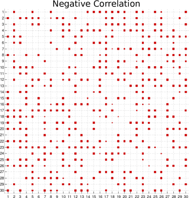Topic 1: get, really, like, just, know, hes, think, dont, thing, say

Topic 2: percent, year, said, last, prices, economy, quarter, home, economic, housing

Topic 3: day, mother, life, family, father, mothers, love, time, home, fathers

Topic 4: make, like, dont, youre, people, time, get, see, love, just

Topic 5: delegates, obama, superdelegates, democratic, party, states, convention, primaries, michigan

Topic 6: mccain, john, mccains, republican, campaign, bush, hes, just, senator, said

Topic 7: show, song, said, music, night, first, david, like, simon, performance

Topic 8: clinton, obama, clintons, hillary, nomination, democratic, barack, race, obamas, supporters

Topic 9: hillary, obama, president, candidate, shes, win, time, democratic, hillarys, running

Topic 10: iran, nuclear, weapons, states, said, united, attack, bush, president, iranian

Topic 11: democrats, republican, republicans, election, democratic, house, vote, states, gop, political

Topic 12: words, word, people, power, like, language, point, written, person, powerful

Topic 13: iraq, war, american, bush, afghanistan, years, petraeus, troops, new, mission

Topic 14: voters, obama, indiana, carolina, north, clinton, polls, primary, democratic, pennsylvania

Topic 15: america, american, nation, country, americans, history, civil, years, king, national

Topic 16: said, city, people, two, homes, area, water, river, state, officials

Topic 17: media, news, story, coverage, television, new, public, journalism, broadcast, channel

Topic 18: israel, peace, israeli, east, hamas, palestinian, state, arab, middle, israels

Topic 19: poll, chance, gallup, degrees, winning, results, tracking, general, election, august

Topic 20: said, iraqi, government, forces, baghdad, city, shiite, security, sadr, minister

Topic 21: senator, obama, obamas, people, clinton, pennsylvania, comments, bitter, remarks, negative

Topic 22: rights, law, court, justice, constitution, supreme, right, laws, courts, constitutional

Topic 23: company, said, billion, yahoo, stock, share, inc, deal, microsoft, shares

Topic 24: health, care, families, insurance, working, pay, help, americans, plan, people

Topic 25: white, race, voters, obama, virginia, west, percent, states, whites, win

Topic 26: wright, obama, rev, jeremiah, pastor, obamas, reverend, political, said, black

Topic 27: tax, government, economic, spending, taxes, cuts, economy, budget, federal, people

Topic 28: study, cancer, found, drugs, age, risk, drug, heart, brain, medical

Topic 29: people, man, black, america, didnt, god, hope, know, years, country

Topic 30: global, climate, warming, change, energy, countries, new, carbon, environmental, emissions

Figure 5: Huffington Post: The ten most probable words from the 30 most popular topics. At top are the positive and negative correlation coefficients for these topics calculated by taking the dot product of the topic locations, $\ell_{k}^{T}\ell_{k^{\prime}}$ (separated for clarity).

Topic 1: manager, science, fax, advertising, aaas, sales, recruitment, member, associate, washington

Topic 2: research, science, funding, scientists, university, universities, government, program, year

Topic 3: fault, plate, earthquake, earthquakes, zone, crust, seismic, fig, crustal, large

Topic 4: hiv, virus, infection, infected, viral, viruses, human, immunodeficiency, aids, disease

Topic 5: species, forest, forests, conservation, ecosystems, fish, natural, land, tropical, ecological

Topic 6: climate, changes, temperature, change, global, atmospheric, carbon, years, year, variability

Topic 7: cells, immune, cell, antigen, response, responses, mice, lymphocytes, antibody, specific

Topic 8: transcription, binding, dna, transcriptional, promoter, polymerase, factors, site, protein

Topic 9: says, university, just, colleagues, team, like, researchers, meeting, new, end

Topic 10: structure, residues, helix, binding, two, fig, helices, side, three, helical

Topic 11: proteins, protein, membrane, ras, gtp, binding, bound, transport, guanosine, membranes

Topic 12: pressure, temperature, high, phase, pressures, temperatures, experiments, gpa, melting

Topic 13: rna, mrna, site, splicing, rnas, pre, intron, base, cleavage, nucleotides

Topic 14: protein, cdna, fig, sequence, lane, purified, human, lanes, clone, gel

Topic 15: kinase, protein, phosphorylation, kinases, activity, activated, signaling, camp, pathway

Topic 16: university, students, says, faculty, graduate, women, science, professor, job, lab

Topic 17: new, says, university, years, human, humans, ago, found, modern, first

Topic 18: researchers, found, called, says, team, work, colleagues, new, university, protein

Topic 19: isotopic, carbon, oxygen, isotope, water, values, ratios, organic, samples, composition

Topic 20: disease, patients, diseases, gene, alzheimers, cause, mutations, syndrome, protein, genetic

Topic 21: aids, vaccine, new, researchers, vaccines, trials, people, research, clinical, patients

Topic 22: receptor, receptors, binding, ligand, transmembrane, surface, signal, hormone, extracellular

Topic 23: cells, cell, bone, human, marrow, stem, types, line, lines, normal

Topic 24: united, states, countries, international, world, development, japan, european, nations, europe

Topic 25: proteins, protein, yeast, two, domain, sequence, conserved, function, amino, family

Topic 26: letters, mail, web, end, new, org, usa, science, full, letter

Topic 27: amino, acid, peptide, acids, peptides, residues, sequence, binding, sequences, residue

Topic 28: species, evolution, evolutionary, phylogenetic, biology, organisms, history, different, evolved

Topic 29: ocean, sea, pacific, water, atlantic, marine, deep, surface, north, waters

Topic 30: gene, genes, development, genetic, mouse, function, expressed, expression, molecular, product

Figure 6: Science: The ten most probable words from the 30 most popular topics. At top are the positive and negative correlation coefficients for these topics calculated by taking the dot product of the topic locations, $\ell_{k}^{T}\ell_{k^{\prime}}$ (separated for clarity).

Figure 7: Several example document searches for Science. The first document is the query document, followed by the most similar documents according to the cosine similarity measure on their locations (given at left).

As we discussed in Section 3.4, the underlying vectors $u_{m}\in\mathbb{R}^{d}$ associated with each document can be used for retrieval applications. In Figure 7, we show recommendation lists for a 16,000 document corpus of the journal Science obtained using these underlying document locations. We use the cosine similarity between two documents for ranking, which for documents $i$ and $j$ is equal to $u_{i}^{T}u_{j}/\|u_{i}\|_{2}\|u_{j}\|_{2}$. We show several lists of recommended articles based on randomly selected query articles. These lists show that, as with the underlying correlations learned between the topics, DILN learns a meaningful relationship between the documents as well, which is useful for navigating text corpora.

Figure 8: Stochastic variational inference results on Nature. The number of documents processed is shown in log scale. We observe improved performance for all algorithms as $\kappa$ decreases, and note that DILN is able to obtain a level of performance not reached by HDP and LDA as a function of parameter settings.

Stochastic variational inference

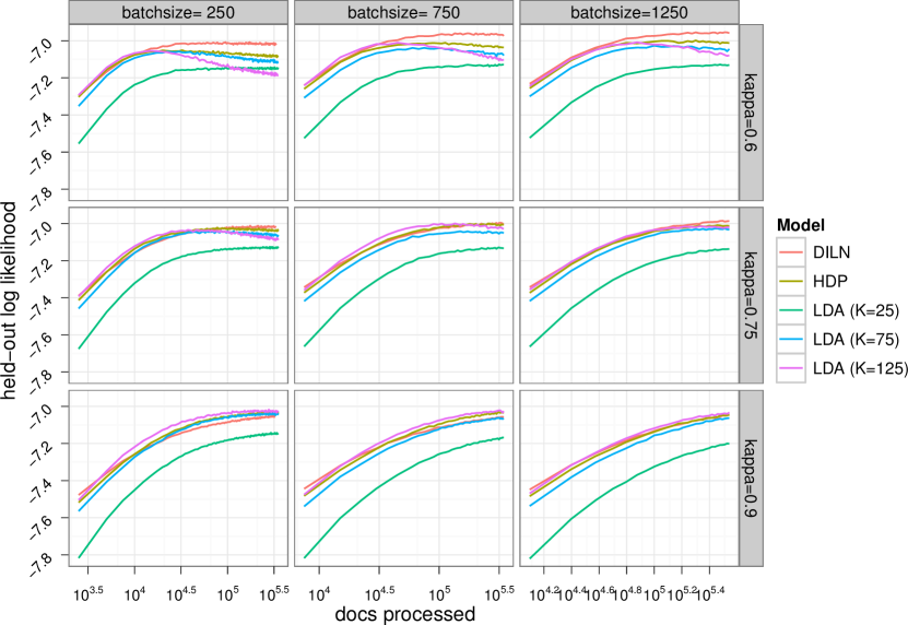
We compare stochastic DILN with stochastic HDP and online LDA using 352,549 documents from Nature. As for batch inference, we can obtain a stochastic inference algorithm for the HDP as a special case of stochastic DILN. In DILN, we again use a latent space of $d=20$ dimensions for the component locations and set the location variance parameter to $c=1/20$. We truncate the models at $200$ topics, and we evaluate performance for $K\in\{25,75,125\}$ topics with stochastic inference for LDA (Hoffman, Blei and Bach, 2010). As we discussed in Section 4.2, we use a step sequence of $\rho_{t}=(\zeta+t)^{-\kappa}$. We set $\zeta=25$, and run the algorithm for $\kappa\in\{0.6,0.75,0.9\}$. We explored various batch sizes, running the algorithm for $|B_{t}|\in\{250,750,1250\}$. Following Hoffman, Blei and Bach (2010), we set the topic Dirichlet hyperparameters to $\gamma_{0}=0.01$.

For testing, we held out $10,000$ randomly selected documents from the corpus. We measure the performance of the stochastic models after every $10$th batch. Within each batch, we run several iterations of local variational inference to find document-specific parameters. We update corpus-level parameters when the change in the average per-document topic distributions falls below a threshold. On average, roughly ten document-level iterations were run for each corpus-level update.

Figure 9: Stochastic learning of Nature. The values of $\hat{\alpha}$ and $\hat{\beta}$ as a function of number of documents seen for batch size equal to 750 and learning rate $\kappa=0.6$.

Figure 10: Stochastic learning of Nature. (left) Correlations between 100 randomly selected pairs of topics as a function of documents seen. (right) The empirical word count from the posteriors of the top 50 topics after the final iteration. Approximately 50 of the 200 topics are used.

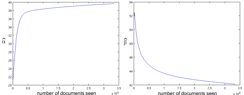
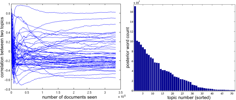
Figure 8 illustrates the results. In this figure, we show the per-word held-out perplexity as a function of the number of documents seen by the algorithm. From these plots we see that a slower decay in the step size improves performance. Especially for DILN, we see that performance improves significantly as the decay $\kappa$ decreases, since more information is being used from later documents in finding a maximum of the variational objective function. Slower decays are helpful because more parameters are being fitted by DILN than by the HDP and LDA. We observed that as $\kappa$ increases a less detailed correlation structure was found; this accounts for the decrease in performance.

Topic 1: author, facts, original, written, hand, text, think, himself, pages, mind

Topic 2: war, england, carried, death, french, german, issued, great-britain, sent, works

Topic 3: equation, flow, sample, average, mantle, rates, distribution, zone, ratios, calculated

Topic 4: million, scientists, policy, britain, social, economic, technology, political, project, organization

Topic 5: gene, genes, expression, mutant, wild-type, sequence, supplementary, embryos, mutants, clones

Topic 6: glass, tube, colour, due, substance, rays, apparatus, substances, action-of, series

Topic 7: serum, labelled, fraction, anti, purified, buffer, fractions, rabbit, extract, extracts

Topic 8: feet, rocks, island, specimens, sea, coast, islands, river, land, geological

Topic 9: membrane, enzyme, concentration, glucose, inhibition, calcium, release, phosphate

Topic 10: population, evolution, selection, genetic, environment, evolutionary, food, birds, breeding

Topic 11: college, secretary, council, cambridge, department, engineering, assistant, mathematics

Topic 12: frequency, wave, spectrum, electron, absorption, band, electrons, optical, signal, peak

Topic 13: binding, proteins, residues, peptide, chain, amino-acid, domain, terminal, sequence

Topic 14: dna, rna, sequence, sequences, mrna, poly, fragments, synthesis, fragment, phage

Topic 15: molecules, compounds, oxygen, molecule, reactions, formation, ion, ions, oxidation, compound

Topic 16: the-sun, solar, the-earth, motion, observatory, stars, comet, star, night, planet

Topic 17: techniques, materials, applications, reader, design, basic, service, computer, fundamental

Topic 18: crystal, structures, unit, orientation, ray, diffraction, patterns, lattice, layer, symmetry

Topic 19: vol, museum, plates, india, journal, ltd, net, indian, series, washington

Topic 20: sea, ice, ocean, depth, deep, the-earth, climate, sediments, earth, global

Topic 21: you, says, her, she, researchers, your, scientists, colleagues, get, biology

Topic 22: mice, anti, mouse, tumour, antigen, antibody, cancer, tumours, antibodies, antigens

Topic 23: disease, blood, bacteria, patients, drug, diseases, clinical, drugs, bacterial, host

Topic 24: radio, ray, emission, flux, stars, disk, sources, star, galaxies, galaxy

Topic 25: brain, receptor, receptors, responses, stimulation, response, stimulus, cortex, synaptic, stimuli

Topic 26: rats, liver, tissue, blood, dose, injection, rat, plasma, injected, hormone

Topic 27: royal, lecture, lectures, engineers, royal-society, hall, institution-of, society-at, annual, january

Topic 28: virus, cultures, culture, medium, infected, infection, viral, viruses, agar, colonies

Topic 29: heat, oil, coal, electric, electricity, electrical, lead, supply, steam, tons

Topic 30: particles, particle, electron, proton, neutron, protons, mev, force, scattering, nuclei

Topic 31: education, universities, training, schools, teaching, teachers, courses, colleges, grants, student

Topic 32: nuclear, radiation, irradiation, radioactive, uranium, fusion, reactor, storage, damage

Topic 33: iron, copper, steel, metals, milk, aluminium, alloys, silicon, ore, haem

Topic 34: soil, nitrogen, leaves, land, agricultural, agriculture, nutrient, yield, growing, content

Topic 35: chromosome, nuclei, hybrid, chromatin, mitotic, division, mitosis, chromosomal, somatic

Topic 36: pulse, spin, magnetic-field, pulses, polarization, orbital, decay, dipole, pulsar, polarized

Topic 37: atoms, quantum, atom, einstein, classical, photon, relativity, bohr, quantum-mechanics

Topic 38: strain, stress, strains, deformation, shear, stresses, failure, viscosity, mechanical, stressed

Topic 39: medical, health, medicine, tuberculosis, schools, education, teaching, infection, bacilli, based

Topic 40: adult, females, males, mating, mature, progeny, adults, maturation, aggressive, matings

Figure 11: Stochastic DILN after one pass through the Nature corpus. The upper left figure shows the projected topic locations with + marking the origin. The upper right figure shows topic correlations. We list the ten most probable for the first 40 topics.

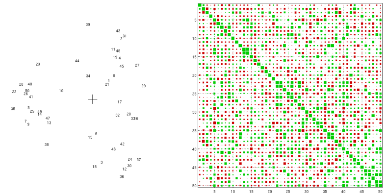
In Figure 11 we show the model after one pass through the Nature corpus. The upper left figure shows the locations of the top 50 topics projected from $\mathbb{R}^{20}$. These locations are rough approximations since the singular values were large for higher dimensions. The upper right figure shows the correlations between the topics. Below these two plots, we show the ten most probable words from the 50 most probable topics. In Figure 10 we show $\hat{\alpha}$ and $\hat{\beta}$ as a function of the number of documents seen by the model. In Figure 10 we show the correlations between 100 pairs of topics chosen at random; these are also shown as a function of the number of documents seen. In general, these plots indicate that the parameters are far along in the process of converging to a local optimum after just one pass through the entire corpus. Also shown in Figure 10 is the empirical word count per topic (that is, the values $\sum_{m,n}\mathbb{I}(C_{n}^{(m)}=k)$ as a function of $k$) after the final iteration of the first pass through the data. We see that the model learns approximately 50 topics out of the 200 initially supplied. All results are shown for a batch size of 750.

Stochastic DILN vs batch DILN

We also compare stochastic and batch inference for DILN to show how stochastic inference can significantly speed up the inference process, while still giving results as good as batch inference. We again use the Nature corpus. For stochastic inference, we use a subset of size $|B_{t}|=1000$ and a step of $(1+t)^{-0.75}$. For batch inference, we use a randomly selected subset of documents, performing experiments on corpus size $M\in\{25000,50000,100000\}$. All algorithms used the same test set and testing procedure, as discussed in Section 5.1. All experiments were run on the same computer to allow for fair time comparisons.

Figure 12: A comparison of stochastic and batch inference for DILN using the Nature corpus. Results are shown as a function of time (log scale). Stochastic inference achieves a good posterior approximation significantly faster than batch inference, which pays for improved performance with an increasing runtime.

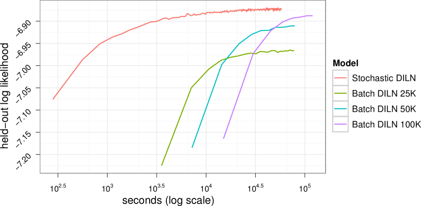
In Figure 12, we plot the held-out per-word log likelihood as a function of time. We measured performance every tenth iteration to construct each curve. The stochastic inference curve represents roughly six passes through the entire corpus. For batch inference, we see that performance improves significantly as the sub-sampled batch size increases. However, this improvement is paid for with an increasing runtime. Stochastic inference is much faster, but still performs as well as batch in predicting test documents.

6 Discussion

We have presented the discrete infinite logistic normal distribution, a Bayesian nonparametric prior for mixed-membership models. DILN overcomes the hidden assumptions of the HDP and explicitly models correlation structure between the mixing weights at the group level. We showed how using the second parameter of the gamma process representation of the hierarchical Dirichlet process achieves this by varying per-component according to an exponentiated Gaussian process. This Gaussian process is defined on latent component locations added to the hierarchical structure of the HDP.

Using batch variational Bayesian inference, we showed an improvement in predictive ability over the HDP and the CTM in a topic modeling application. Furthermore, we showed how this algorithm can be modified to obtain a new variational inference algorithm for HDPs based on the gamma process. We then extended the model to the stochastic inference setting, which allows for fast analysis of much larger corpora.

DILN can be useful in other modeling frameworks. For example, hidden Markov models can be viewed as a collection of mixture models that are defined over a shared set of parameters, where state transitions follow a Markov transition rule. Teh et al. (2006) showed how the HDP can be applied to the HMM to allow for infinite state support, thus creating a nonparametric hidden Markov model, where the number of underlying states is inferred. DILN can be adapted to this problem as well, in this case modeling correlations between state transition probabilities.

7 Appendix

7.1 Proof of almost sure finiteness of $\sum_{i=1}^{\infty}Z_{i}\mathrm{e}^{w_{i}}$

We drop the group index $m$ and define $w_{i}:=W(\ell_{i})$. The normalizing constant for DILN, prior to absorbing the scaling factor within the gamma distribution, is $S:=\sum_{i=1}^{\infty}Z_{i}\mathrm{e}^{w_{i}}$. We first show that this value is finite almost surely when the Gaussian process has bounded mean and covariance functions. This case would apply for example when using a Gaussian kernel. We then give a proof for the kernel in Section 3.4 when the value of $c<1$.

Let $S_{T}:=\sum_{i=1}^{T}Z_{i}\mathrm{e}^{w_{i}}$. It follows that $S_{1}\leq\dots\leq S_{T}\leq\dots\leq S$ and $S=\lim_{T\to\infty}S_{T}$. To prove that $S$ is finite almost surely, we only need to prove that $\mathbb{E}[S]$ is finite. From the monotone convergence theorem, we have that $\mathbb{E}[S]=\lim_{T\to\infty}\mathbb{E}[S_{T}]$. Furthermore, $\mathbb{E}[S_{T}]$ can be upper bounded as follows,

$$\mathbb{E}[S_{T}]=\textstyle\sum_{i=1}^{T}\mathbb{E}[Z_{i}]\mathbb{E}[\mathrm{e}^{w_{i}}]\leq\mathrm{e}^{\max_{i}(\mu_{i}+\frac{1}{2}\sigma_{i}^{2})}\textstyle\sum_{i=1}^{T}\mathbb{E}[Z_{i}].$$ (42)

$\mathbb{E}[S]$ is therefore upper bounded by $\beta\mathrm{e}^{\max_{i}(\mu_{i}+\frac{1}{2}\sigma_{i}^{2})}$ and $S$ is finite almost surely.

For the kernel in Section 3.4, we prove that $\mathbb{E}[S]<\infty$ when $c<1$. We only focus on this case since values of $c\geq 1$ are larger than we are interested in for our application. For example, given that $\ell\in\mathbb{R}^{d}$ and $\ell\sim\mathrm{Normal}(0,cI_{d})$, it follows that $\mathbb{E}[\ell^{T}\ell]=dc$, which is the expected variance of the Gaussian process at this location. In our applications, we set $c=1/d$, which is less than one when $d>1$. As above, we have

$$\mathbb{E}[S_{T}]=\textstyle\sum_{i=1}^{T}\mathbb{E}[Z_{i}]\mathbb{E}[\mathrm{e}^{\ell_{i}^{T}u}]=\textstyle\sum_{i=1}^{T}\beta p_{i}\mathbb{E}[\mathrm{e}^{\frac{c}{2}u^{T}u}].$$ (43)

Since $u\sim\mathrm{Normal}(0,I_{d})$, this last expectation is finite when $c<1$, and therefore the limit $\lim_{T\rightarrow\infty}\mathbb{E}[S_{T}]$ is also finite.

7.2 Variational inference for normalized gamma measures

In DILN, and normalized gamma models in general, the expectation of the log of the normalizing constant, $\mathbb{E}_{Q}[\ln\sum_{k}Z_{k}]$, is intractable. We present a method for approximate variational Bayesian inference for these models. A Taylor expansion on this term about a particular point allows for tractable expecations, while still preserving the lower bound on the log-evidence of the model. Since the log function is concave, the negative of this function can be lower bounded by a first-order Taylor expansion,

$$-\mathbb{E}_{Q}\left[\ln\sum_{k=1}^{T}Z_{k}\right]\geq-\ln\xi-\frac{\sum_{k}\mathbb{E}_{Q}[Z_{k}]-\xi}{\xi}.$$ (44)

We have dropped the group index $m$ for clarity. A new term $\xi$ is introduced into the model as an auxiliary parameter. Changing this parameter changes the tightness of the lower bound, and in fact, it can be removed by permanently tightening it,

$$\xi=\sum_{k=1}^{T}\mathbb{E}_{Q}[Z_{k}].$$ (45)

In this case $\mathbb{E}_{Q}[\ln\sum_{k}Z_{k}]$ is replaced with $\ln\sum_{k}\mathbb{E}_{Q}[Z_{k}]$ in the variational objective function. We do not do this, however, since retaining $\xi$ in DILN allows for analytical parameter updates, while using Equation (45) requires gradient methods. These analytical updates result in an algorithm that is significantly faster. For example, inference for the corpora considered in this paper ran approximately five times faster.

Because this property extends to variational inference for all mixture models using the normalized gamma construction, most notably the HDP, we derive these updates using a generic parameterization of the gamma distribution, $\mathrm{Gamma}(a_{k},b_{k})$. The posterior of $Z_{1:T}$ in this model is proportional to

$$p(Z_{1:T}|C_{1:N},a_{1:T},b_{1:T})\propto\left[\prod_{n=1}^{N}\prod_{k=1}^{T}\left(\frac{Z_{k}}{\sum_{j}Z_{j}}\right)^{\mathbb{I}(C_{n}=k)}\right]\left[\prod_{k=1}^{T}Z_{k}^{a_{k}-1}\mathrm{e}^{-b_{k}Z_{k}}\right].$$ (46)

Under a factorized $Q$ distribution, the variational lower bound at nodes $Z_{1:T}$ is

$$\mathbb{E}_{Q}[\ln p(Z_{1:T}|-)]+\mathbb{H}[Q] = \sum_{n=1}^{N}\sum_{k=1}^{T}\mathbb{P}_{Q}(C_{n}=k)\mathbb{E}_{Q}[\ln Z_{k}]-N\mathbb{E}_{Q}\left[\ln\sum_{k=1}^{T}Z_{k}\right]$$ (47)

$$+\sum_{k=1}^{T}(\mathbb{E}_{Q}[a_{k}]-1)\mathbb{E}_{Q}[\ln Z_{k}]-\sum_{k=1}^{T}\mathbb{E}_{Q}[b_{k}]\mathbb{E}_{Q}[Z_{k}]$$

$$+\sum_{k=1}^{T}\mathbb{H}[Q(Z_{k})]\,+\,\mbox{const.}$$

The intractable term, $-N\mathbb{E}_{Q}[\ln\sum_{k}Z_{k}]$, is replaced with the bound in Equation (44).

Rather than calculate for a specific $q$ distribution on $Z_{k}$, we use the procedure discussed by Winn and Bishop (2005) for finding the optimal form and parameterization of a given $q$: We exponentiate the variational lower bound in Equation (47) with all expectations involving the parameter of interest not taken. For $Z_{k}$, this gives

$$q(Z_{k}) \propto \mathrm{e}^{\mathbb{E}_{Q_{-Z_{k}}}[\ln p(Z_{k}|C_{1:N},a_{1:T},b_{1:T})]}$$ (48)

$$\propto Z_{k}^{\mathbb{E}_{Q}[a_{k}]+\sum_{n=1}^{N}\mathbb{P}_{Q}(C_{n}=k)-1}~{}\mathrm{e}^{-(\mathbb{E}_{Q}[b_{k}]+N/\xi)Z_{k}}.$$

Therefore, the optimal $q$ distribution for $Z_{k}$ is $q(Z_{k})=\mathrm{Gamma}(Z_{k}|a^{\prime}_{k},b^{\prime}_{k})$ with $a^{\prime}_{k}=\mathbb{E}_{Q}[a_{k}]+\sum_{n=1}^{N}\mathbb{P}_{Q}(C_{n}=k)$ and $b^{\prime}_{k}=\mathbb{E}_{Q}[b_{k}]+N/\xi$. The specific values of $a^{\prime}_{k}$ and $b^{\prime}_{k}$ for DILN are given in Equation (4.1).

References

- Airoldi et al. (2008) {barticle}[author] \bauthor\bsnmAiroldi, \bfnmE.\binitsE., \bauthor\bsnmBlei, \bfnmD.\binitsD., \bauthor\bsnmFienberg, \bfnmS.\binitsS. and \bauthor\bsnmXing, \bfnmE.\binitsE. (\byear2008). \btitleMixed Membership Stochastic Blockmodels. \bjournalJournal of Machine Learning Research \bvolume9 \bpages1981–2014. \endbibitem
- Aitchison (1982) {barticle}[author] \bauthor\bsnmAitchison, \bfnmJ.\binitsJ. (\byear1982). \btitleThe statistical analysis of compositional data. \bjournalJournal of the Royal Statistical Society, Series B \bvolume44 \bpages139–177. \endbibitem
- Armagan and Dunson (2011) {barticle}[author] \bauthor\bsnmArmagan, \bfnmA.\binitsA. and \bauthor\bsnmDunson, \bfnmD. B.\binitsD. B. (\byear2011). \btitleSparse variational analysis of large longitudinal data sets. \bjournalStatistics & Probability Letters \bvolume81 \bpages1056-1062. \endbibitem
- Asuncion et al. (2009) {binproceedings}[author] \bauthor\bsnmAsuncion, \bfnmA.\binitsA., \bauthor\bsnmWelling, \bfnmM.\binitsM., \bauthor\bsnmSmyth, \bfnmP.\binitsP. and \bauthor\bsnmTeh, \bfnmY. W.\binitsY. W. (\byear2009). \btitleOn smoothing and inference for topic models. In \bbooktitleUncertainty in Artificial Intelligence. \endbibitem
- Blackwell and MacQueen (1973) {barticle}[author] \bauthor\bsnmBlackwell, \bfnmD.\binitsD. and \bauthor\bsnmMacQueen, \bfnmJ. B.\binitsJ. B. (\byear1973). \btitleFerguson Distributions Via Pólya Urn Schemes. \bjournalAnnals of Statistics \bvolume1 \bpages353-355. \endbibitem
- Blei and Jordan (2005) {barticle}[author] \bauthor\bsnmBlei, \bfnmD.\binitsD. and \bauthor\bsnmJordan, \bfnmM.\binitsM. (\byear2005). \btitleVariational inference for Dirichlet process mixtures. \bjournalJournal of Bayesian Analysis \bvolume1 \bpages121–144. \endbibitem
- Blei and Lafferty (2007) {barticle}[author] \bauthor\bsnmBlei, \bfnmD.\binitsD. and \bauthor\bsnmLafferty, \bfnmJ.\binitsJ. (\byear2007). \btitleA correlated topic model of Science. \bjournalAnnals of Applied Statistics \bvolume1 \bpages17–35. \endbibitem
- Blei and Lafferty (2009) {bincollection}[author] \bauthor\bsnmBlei, \bfnmD.\binitsD. and \bauthor\bsnmLafferty, \bfnmJ.\binitsJ. (\byear2009). \btitleTopic Models. In \bbooktitleText Mining: Theory and Applications (\beditor\bfnmA.\binitsA. \bsnmSrivastava and \beditor\bfnmM.\binitsM. \bsnmSahami, eds.) \bpublisherTaylor and Francis. \endbibitem
- Blei, Ng and Jordan (2003) {barticle}[author] \bauthor\bsnmBlei, \bfnmD.\binitsD., \bauthor\bsnmNg, \bfnmA.\binitsA. and \bauthor\bsnmJordan, \bfnmM.\binitsM. (\byear2003). \btitleLatent Dirichlet allocation. \bjournalJournal of Machine Learning Research \bvolume3 \bpages993–1022. \endbibitem
- Dawid (1981) {barticle}[author] \bauthor\bsnmDawid, \bfnmA. P.\binitsA. P. (\byear1981). \btitleSome matrix-variate distribution theory: Notational considerations and a Bayesian application. \bjournalBiometrika \bvolume68 \bpages265-274. \endbibitem
- Duan, Guindani and Gelfand (2007) {barticle}[author] \bauthor\bsnmDuan, \bfnmJ. A.\binitsJ. A., \bauthor\bsnmGuindani, \bfnmM.\binitsM. and \bauthor\bsnmGelfand, \bfnmA. E.\binitsA. E. (\byear2007). \btitleGeneralized spatial Dirichlet process models. \bjournalBiometrika \bvolume94 \bpages809-825. \endbibitem
- Dunson and Park (2008) {barticle}[author] \bauthor\bsnmDunson, \bfnmD.\binitsD. and \bauthor\bsnmPark, \bfnmJ. H.\binitsJ. H. (\byear2008). \btitleKernel stick-breaking processes. \bjournalBiometrika \bvolume95 \bpages307-323. \endbibitem
- Dunson, Pillai and Park (2007) {barticle}[author] \bauthor\bsnmDunson, \bfnmD. B.\binitsD. B., \bauthor\bsnmPillai, \bfnmN.\binitsN. and \bauthor\bsnmPark, \bfnmJ. H.\binitsJ. H. (\byear2007). \btitleBayesian density regression. \bjournalJournal of the Royal Statistical Society \bvolume69 \bpages163-183. \endbibitem
- Erosheva, Fienberg and Lafferty (2004) {barticle}[author] \bauthor\bsnmErosheva, \bfnmE.\binitsE., \bauthor\bsnmFienberg, \bfnmS.\binitsS. and \bauthor\bsnmLafferty, \bfnmJ.\binitsJ. (\byear2004). \btitleMixed-membership models of scientific publications. \bjournalProceedings of the National Academy of Science \bvolume97 \bpages11885-11892. \endbibitem
- Erosheva, Fienberg and Joutard (2007) {barticle}[author] \bauthor\bsnmErosheva, \bfnmE.\binitsE., \bauthor\bsnmFienberg, \bfnmS.\binitsS. and \bauthor\bsnmJoutard, \bfnmC.\binitsC. (\byear2007). \btitleDescribing Disability Through Individual-Level Mixture Models for Multivariate Binary Data. \bjournalAnnals of Applied Statistics \bvolume1 \bpages346-384. \endbibitem
- Escobar and West (1995) {barticle}[author] \bauthor\bsnmEscobar, \bfnmMichael D.\binitsM. D. and \bauthor\bsnmWest, \bfnmMike\binitsM. (\byear1995). \btitleBayesian density estimation and inference using mixtures. \bjournalJournal of the American Statistical Association \bvolume90 \bpages577-588. \endbibitem
- Ferguson (1973) {barticle}[author] \bauthor\bsnmFerguson, \bfnmT.\binitsT. (\byear1973). \btitleA Bayesian analysis of some nonparametric problems. \bjournalThe Annals of Statistics \bvolume1 \bpages209-230. \endbibitem
- Ferguson (1983) {bincollection}[author] \bauthor\bsnmFerguson, \bfnmT. S.\binitsT. S. (\byear1983). \btitleBayesian density estimation by mixtures of normal distributions. In \bbooktitleRecent Advances in Statistics, (\beditor\bfnmM. H.\binitsM. H. \bsnmRizvi, \beditor\bfnmJ.\binitsJ. \bsnmRustagi and \beditor\bfnmD.\binitsD. \bsnmSiegmund, eds.) \bvolume155 \bpages287-302. \bpublisherAcademic Press. \endbibitem
- Gelfand, Kottas and MacEachern (2005) {barticle}[author] \bauthor\bsnmGelfand, \bfnmA. E.\binitsA. E., \bauthor\bsnmKottas, \bfnmA.\binitsA. and \bauthor\bsnmMacEachern, \bfnmS. N.\binitsS. N. (\byear2005). \btitleBayesian nonparametric spatial modeling with Dirichlet process mixing. \bjournalJournal of the American Statistical Association \bvolume100 \bpages1021-1035. \endbibitem
- Griffin and Steel (2006) {barticle}[author] \bauthor\bsnmGriffin, \bfnmJ. E.\binitsJ. E. and \bauthor\bsnmSteel, \bfnmM. F. J.\binitsM. F. J. (\byear2006). \btitleOrder-based dependent Dirichlet processes. \bjournalJournal of the American Statistical Association \bvolume101 \bpages179-194. \endbibitem
- Griffin and Walker (2010) {barticle}[author] \bauthor\bsnmGriffin, \bfnmJim E.\binitsJ. E. and \bauthor\bsnmWalker, \bfnmStephen G.\binitsS. G. (\byear2010). \btitlePosterior Simulation of Normalized Random Measure Mixtures. \bjournalJournal of Computational and Graphical Statistics \bvolume0 \bpages1-19. \endbibitem
- Griffiths and Steyvers (2004) {barticle}[author] \bauthor\bsnmGriffiths, \bfnmT.\binitsT. and \bauthor\bsnmSteyvers, \bfnmM.\binitsM. (\byear2004). \btitleFinding scientific topics. \bjournalProceedings of the National Academy of Science. \endbibitem
- Hastings (1970) {barticle}[author] \bauthor\bsnmHastings, \bfnmW. K.\binitsW. K. (\byear1970). \btitleMonte Carlo sampling methods using Markov chains and their applications. \bjournalBiometrika \bvolume57 \bpages97-109. \endbibitem
- Hoffman, Blei and Bach (2010) {binproceedings}[author] \bauthor\bsnmHoffman, \bfnmM.\binitsM., \bauthor\bsnmBlei, \bfnmD.\binitsD. and \bauthor\bsnmBach, \bfnmF.\binitsF. (\byear2010). \btitleOnline learning for latent Dirichlet allocation. In \bbooktitleAdvances in Neural Information Processing Systems. \endbibitem
- Ishwaran and James (2001) {barticle}[author] \bauthor\bsnmIshwaran, \bfnmH.\binitsH. and \bauthor\bsnmJames, \bfnmL. F.\binitsL. F. (\byear2001). \btitleGibbs sampling methods for stick-breaking priors. \bjournalJournal of the American Statistical Association \bvolume96 \bpages161-173. \endbibitem
- Ishwaran and Zarepour (2002) {barticle}[author] \bauthor\bsnmIshwaran, \bfnmH.\binitsH. and \bauthor\bsnmZarepour, \bfnmM.\binitsM. (\byear2002). \btitleExact and approximate sum representations for the Dirichlet process. \bjournalCanadian Journal of Statistics \bvolume30 \bpages269–283. \endbibitem
- Jordan et al. (1999) {barticle}[author] \bauthor\bsnmJordan, \bfnmM. I.\binitsM. I., \bauthor\bsnmGhahramani, \bfnmZ.\binitsZ., \bauthor\bsnmJaakkola, \bfnmT.\binitsT. and \bauthor\bsnmSaul, \bfnmL. K.\binitsL. K. (\byear1999). \btitleAn introduction to variational methods for graphical models. \bjournalMachine Learning \bvolume37 \bpages183–233. \endbibitem
- Kalli, Griffin and Walker (2011) {barticle}[author] \bauthor\bsnmKalli, \bfnmMaria\binitsM., \bauthor\bsnmGriffin, \bfnmJim\binitsJ. and \bauthor\bsnmWalker, \bfnmStephen\binitsS. (\byear2011). \btitleSlice sampling mixture models. \bjournalStatistics and Computing \bvolume21 \bpages93-105. \endbibitem
- Kingman (1993) {bbook}[author] \bauthor\bsnmKingman, \bfnmJ.\binitsJ. (\byear1993). \btitlePoisson Processes. \bpublisherOxford University Press, USA. \endbibitem
- Kurihara, Welling and Vlassis (2006) {binproceedings}[author] \bauthor\bsnmKurihara, \bfnmKenichi\binitsK., \bauthor\bsnmWelling, \bfnmMax\binitsM. and \bauthor\bsnmVlassis, \bfnmNikos\binitsN. (\byear2006). \btitleAccelerated variational DP mixture models. In \bbooktitleAdvances in Neural Information Processing Systems. \endbibitem
- Lenk (1988) {barticle}[author] \bauthor\bsnmLenk, \bfnmP.\binitsP. (\byear1988). \btitleThe logistic normal distribution for Bayesian, nonparametric, predictive densities. \bjournalJournal of the American Statistical Association \bvolume83 \bpages509–516. \endbibitem
- Liang et al. (2007) {binproceedings}[author] \bauthor\bsnmLiang, \bfnmPercy\binitsP., \bauthor\bsnmPetrov, \bfnmSlav\binitsS., \bauthor\bsnmJordan, \bfnmMichael\binitsM. and \bauthor\bsnmKlein, \bfnmDan\binitsD. (\byear2007). \btitleThe infinite PCFG using hierarchical Dirichlet processes. In \bbooktitleEmpirical Methods in Natural Language Processing. \endbibitem
- Lo (1984) {barticle}[author] \bauthor\bsnmLo, \bfnmA. Y.\binitsA. Y. (\byear1984). \btitleOn a class of Bayesian nonparametric estimates. I. Density estimates. \bjournalAnnals of Statistics \bvolume12 \bpages351-357. \endbibitem
- MacEachern (1999) {binproceedings}[author] \bauthor\bsnmMacEachern, \bfnmS. N.\binitsS. N. (\byear1999). \btitleDependent nonparametric processes. In \bbooktitleASA Proceedings of the Section on Bayesian Statistical Science. \endbibitem
- Muller, Quintana and Rosner (2004) {barticle}[author] \bauthor\bsnmMuller, \bfnmP.\binitsP., \bauthor\bsnmQuintana, \bfnmF.\binitsF. and \bauthor\bsnmRosner, \bfnmG.\binitsG. (\byear2004). \btitleA method for combining inference across related nonparametric Bayesian models. \bjournalJournal of the Royal Statistical Society \bvolume66 \bpages735-749. \endbibitem
- Paisley, Wang and Blei (2011) {binproceedings}[author] \bauthor\bsnmPaisley, \bfnmJ.\binitsJ., \bauthor\bsnmWang, \bfnmC.\binitsC. and \bauthor\bsnmBlei, \bfnmD.\binitsD. (\byear2011). \btitleThe infinite discrete logistic normal distribution for mixed-membership modeling. In \bbooktitleInternational Conference on Artificial Intelligence and Statistics. \endbibitem
- Pritchard, Stephens and Donnelly (2000) {barticle}[author] \bauthor\bsnmPritchard, \bfnmJ.\binitsJ., \bauthor\bsnmStephens, \bfnmM.\binitsM. and \bauthor\bsnmDonnelly, \bfnmP.\binitsP. (\byear2000). \btitleInference of population structure using multilocus genotype data. \bjournalGenetics \bvolume155 \bpages945–959. \endbibitem
- Rao and Teh (2009) {binproceedings}[author] \bauthor\bsnmRao, \bfnmV.\binitsV. and \bauthor\bsnmTeh, \bfnmY. W.\binitsY. W. (\byear2009). \btitleSpatial normalized gamma processes. In \bbooktitleAdvances in Neural Information Processing Systems. \endbibitem
- Rasmussen and Williams (2006) {bbook}[author] \bauthor\bsnmRasmussen, \bfnmC. E.\binitsC. E. and \bauthor\bsnmWilliams, \bfnmC. K. I.\binitsC. K. I. (\byear2006). \btitleGaussian Processes for Machine Learning. \bpublisherMIT press. \endbibitem
- Ren et al. (2011) {barticle}[author] \bauthor\bsnmRen, \bfnmL.\binitsL., \bauthor\bsnmDu, \bfnmL.\binitsL., \bauthor\bsnmCarin, \bfnmL.\binitsL. and \bauthor\bsnmDunson, \bfnmD. B.\binitsD. B. (\byear2011). \btitleLogistic stick-breaking process. \bjournalJournal of Machine Learning Research \bvolume12 \bpages203-239. \endbibitem
- Robbins and Monro (1951) {barticle}[author] \bauthor\bsnmRobbins, \bfnmH.\binitsH. and \bauthor\bsnmMonro, \bfnmS.\binitsS. (\byear1951). \btitleA stochastic approximation method. \bjournalThe Annals of Mathematical Statistics \bvolume22 \bpages400–407. \endbibitem
- Robert and Casella (2004) {bbook}[author] \bauthor\bsnmRobert, \bfnmC. P.\binitsC. P. and \bauthor\bsnmCasella, \bfnmC.\binitsC. (\byear2004). \btitleMonte Carlo Statistical Methods, 2nd Edition. \bpublisherSpringer Texts in Statistics. \endbibitem
- Sato (2001) {barticle}[author] \bauthor\bsnmSato, \bfnmM. A.\binitsM. A. (\byear2001). \btitleOnline model selection based on the variational Bayes. \bjournalNeural Computation \bvolume13 \bpages1649-1681. \endbibitem
- Sethuraman (1994) {barticle}[author] \bauthor\bsnmSethuraman, \bfnmJ.\binitsJ. (\byear1994). \btitleA constructive definition of Dirichlet priors. \bjournalStatistica Sinica \bvolume4 \bpages639–650. \endbibitem
- Teh, Kurihara and Welling (2009) {binproceedings}[author] \bauthor\bsnmTeh, \bfnmY. W.\binitsY. W., \bauthor\bsnmKurihara, \bfnmK.\binitsK. and \bauthor\bsnmWelling, \bfnmM.\binitsM. (\byear2009). \btitleCollapsed variational inference for HDP. In \bbooktitleAdvances in Neural Information Processing Systems. \endbibitem
- Teh et al. (2006) {barticle}[author] \bauthor\bsnmTeh, \bfnmY.\binitsY., \bauthor\bsnmJordan, \bfnmM.\binitsM., \bauthor\bsnmBeal, \bfnmM.\binitsM. and \bauthor\bsnmBlei, \bfnmD.\binitsD. (\byear2006). \btitleHierarchical Dirichlet processes. \bjournalJournal of the American Statistical Association \bvolume101 \bpages1566–1581. \endbibitem
- Wainwright and Jordan (2008) {barticle}[author] \bauthor\bsnmWainwright, \bfnmM. J.\binitsM. J. and \bauthor\bsnmJordan, \bfnmM. I.\binitsM. I. (\byear2008). \btitleGraphical models, exponential families, and variational inference. \bjournalFoundations and Trends in Machine Learning \bvolume1 \bpages1-305. \endbibitem
- Wang, Paisley and Blei (2011) {binproceedings}[author] \bauthor\bsnmWang, \bfnmC.\binitsC., \bauthor\bsnmPaisley, \bfnmJ.\binitsJ. and \bauthor\bsnmBlei, \bfnmD.\binitsD. (\byear2011). \btitleOnline learning for the hierarchical Dirichlet process. In \bbooktitleInternational Conference on Artificial Intelligence and Statistics. \endbibitem
- Winn and Bishop (2005) {barticle}[author] \bauthor\bsnmWinn, \bfnmJ.\binitsJ. and \bauthor\bsnmBishop, \bfnmC.\binitsC. (\byear2005). \btitleVariational message passing. \bjournalJournal of Machine Learning Research \bvolume6 \bpages661–694. \endbibitem