Abstract

In this paper, we present a method for the numerical minimization of the Mumford–Shah functional that is based on the idea of topological asymptotic expansions. The basic idea is to cover the expected edge set with balls of radius $\varepsilon>0$ and use the number of balls, multiplied with $2\varepsilon$, as an estimate for the length of the edge set. We introduce a functional based on this idea and prove that it converges in the sense of $\Gamma$-limits to the Mumford–Shah functional. Moreover, we show that ideas from topological asymptotic analysis can be used for determining where to position the balls covering the edge set. The results of the proposed method are presented by means of two numerical examples and compared with the results of the classical approximation due to Ambrosio and Tortorelli.

Keywords: Topological asymptotic expansion; $\Gamma$-convergence; Mumford-Shah functional; image segmentation.
AMS Classification: 35R35, 65K10, 49M25.

1 Introduction

Let $\Omega$ be a Lipschitz bounded open domain in $\mathbb{R}^{2}$. We assume that a possibly noisy image on $\Omega$ is given, represented by a real-valued, bounded function $f$ on $\Omega$, whose values $f(x)$, $x\in\Omega$, correspond to the intensity of $f$ at the pixel $x$. In order to segment, and denoise at the same time, the image $f$, Mumford and Shah [37] introduced a variational model, which is based on the assumptions that the different “objects” in the image give rise to homogeneous regions that are separated by the objects’ projected silhouettes. Moreover, these silhouettes in general correspond to discontinuities in the image $f$. By this reasoning, they proposed to minimize the functional

$$F(u,K)=\frac{1}{2}\int_{\Omega}(u-f)^{2}\,dx+\frac{\alpha}{2}\int_{\Omega\setminus K}\lvert\nabla u\rvert^{2}\,dx+\beta\mathcal{H}^{1}(K)\,,$$ (1.1)

taking as variables the function $u\in L^{2}(\Omega)$, the denoised image, and the compact set $K\subset\Omega$, the set of edges or silhouettes. Here, the value $F(u,K)$ is set to $+\infty$ if the restriction of the weak derivative $\nabla u$ of $u$ to $\Omega\setminus K$ is not square-integrable. Here, $\mathcal{H}^{1}(K)$ denotes the one-dimensional Hausdorff measure of the set $K$; in the case $K$ is a regular (rectifiable) one-dimensional set, this is precisely its length. The parameters $\alpha$ and $\beta$ that appear in (1.1) are positive constants determining the weight that is put on the regularity of the denoised image $u$ and the length of the edge set $K$.

In order to show the existence of minimizers of the Mumford–Shah functional, a weak formulation depending only on one variable has been introduced by De Giorgi et al. [27]. In their model, the set $K$ is replaced by the jump set $S_{u}$ of the function $u\in SBV(\Omega)$, the space of special function of bounded variation on $\Omega$. Still, this reformulation of the functional provides no method for the actual numerical computation of minimizers. Thus, various approximations of the functional $F$ have been proposed, most of them based on the concept of $\Gamma$-convergence. Ambrosio and Tortorelli [3] proposed a variational model in which they replace the set $S_{u}$ by a continuous function $v$ with values close to $0$ near $S_{u}$, and values close to $1$ away from $S_{u}$. For other approximations of the Mumford–Shah functional in the sense of $\Gamma$-convergence, we refer to Braides et al. [14], where the authors propose approximations by a family of non-local functionals. Approximations by finite-difference schemes, inspired by the original discrete model of Blake and Zisserman [10], have been considered by Chambolle [17, 18], and by finite-elements schemes by Chambolle and Dal Maso [19] or recently by Aubert et al. [6]. In the work by Koepfler et al. [33] and Dal Maso et al. [26], region growing and merging methods have been proposed. For detailed analysis of the Mumford–Shah model, we refer reader to the book by Morel and Solimini [36]. We also refer to the books [7, 40, 41], where some of the above mentioned results are shortly discussed.

In the following, we will show how the problem of minimizing the Mumford–Shah functional $F$ can be approached using ideas of topological asymptotic analysis. In its original formulation (see, e.g., Sokołowski et al. [42], Garreau et al. [30], Feijóo et al. [29]), this theory investigates a variation of a given objective functional depending on some domain in $\mathbb{R}^{n}$ with respect to the subtraction of a small ball from this domain. This variation is a scalar function, called the topological gradient or the topological derivative, and its largest negative values indicate positions, where it is good to remove a small ball. In [5], Amstutz proposed to modify the definition of topological gradient and provide the variation of a given functional with respect to change of certain material properties, and not a domain topology. The topological derivative of an objective functional has also been considered by Giusti et al. [32] in the case of nonlinear elasticity. Recently, topological asymptotic analysis has been also applied by Auroux et al. [8, 9] and by Muszkieta [38] to various problems in image processing.

In order to apply the theory of topological asymptotic expansions, it is necessary that the functional to be minimized depends solely on the set $K$. This can be achieved in the case of the Mumford–Shah functional by noting that the minimizing pair $(u_{0},K_{0})$ is uniquely determined by either of the components $u_{0}$ and $K_{0}$: The set $K_{0}$ coincides with the jump set $S_{u_{0}}$ of the function $u_{0}$. Conversely, $u_{0}$ can be computed from $K_{0}$ by solving the partial differential equation

$$u-\alpha\Delta u =f \text{ in }\Omega\,,$$ (1.2)

$$\frac{\partial u}{\partial n} =0 \text{ in }\partial(\Omega\setminus K_{0})\;.$$

Now consider the functional

$$J(K)=F\bigl{(}u(K),K\bigr{)}\,,$$

where $u(K)$ denotes the solution of (1.2) with $K_{0}$ replaced by $K$. Then the pair $(u(K_{0}),K_{0})$ minimizes the functional $F$, if and only if $J(K_{0})\leq J(K)$ for all $K\subset\Omega$.

The idea is now to use a gradient descent like approach to the minimization of the functional $J$. Starting from an initial guess $K$ of the edge set (for instance $K=\emptyset$), one adds to $K$ those points, whose inclusion would lead to a near to maximal decrease of the cost functional $J$. More precisely, one adjoins to the set $K$ small balls of radius $\varepsilon>0$ centered at the points $x\in\Omega\setminus K$ and tries to compute an asymptotic expansion of the form

$$J\bigl{(}K\cup B_{\varepsilon}(x)\bigr{)}-J(K)=c(\varepsilon)G_{K}(x)+o\bigl{(}c(\varepsilon)\bigr{)}$$

for some functions $c\colon\mathbb{R}_{>0}\to\mathbb{R}_{>0}$ and $G_{K}\colon\Omega\setminus K\to\mathbb{R}$. Those $x\in\Omega\setminus K$ for which $G_{K}$ attains the largest negative values are then added to the set $K$. This process is iterated, until the function $G_{K}$ becomes non-negative everywhere.

In the case of the Mumford–Shah functional, this procedure cannot applied directly, because the functional is infinite whenever $K$ contains a set of positive Lebesgue measure. We therefore propose to use a different, though related, functional for the computation of the asymptotic expansion, which is based on an approximation of the one-dimensional Hausdorff measure: The number of balls of radius $\varepsilon>0$ that are required to cover a set $K$, multiplied with $2\varepsilon$, provides a good estimate of $\mathcal{H}^{1}(K)$ for $\varepsilon$ small enough and $K$ sufficiently regular. In the following, we introduce this approximating functional $J_{\varepsilon,\kappa}$. However, because we later prove the $\Gamma$-convergence of this functional to $F$, it is necessary to let $J_{\varepsilon,\kappa}$ depend on two functions, the function $u$ and a piecewise constant edge indicator function $v$:

For each finite set $Y\subset\mathbb{R}^{2}$ and each $0<\kappa<1$ we define the function $v_{Y,\kappa}\colon\Omega\to\mathbb{R}$ by

$$v_{Y,\kappa}(x):=\begin{cases}\kappa&\text{ if }x\in\bigcup_{y\in Y}B_{\varepsilon}(y)\,,\\ 1&\text{ else.}\end{cases}$$

For every $v\in L^{2}(\Omega)$ we define

$$m_{\varepsilon,\kappa}(v):=\inf\bigl{\{}\mathcal{H}^{0}(Y):Y\subset\mathbb{R}^{2},\ v=v_{Y,\kappa}\bigr{\}}\;.$$

Here we set $m_{\varepsilon,\kappa}(v):=+\infty$, if $v\neq v_{Y,\kappa}$ for any $Y\subset\mathbb{R}^{2}$. Note that, for a given function $v$, there might exist different sets $Y\subset\mathbb{R}^{2}$ such that $v=v_{Y,\kappa}$.

Finally, we introduce the family of functionals $J_{\varepsilon,\kappa}\colon L^{2}(\Omega)\times L^{2}(\Omega)\to[0,+\infty]$, defined by

$$J_{\varepsilon,\kappa}(u,v):=\frac{1}{2}\int_{\Omega}(u-f)^{2}\,dx+\frac{\alpha}{2}\int_{\Omega}v\lvert\nabla u\rvert^{2}\,dx+2\beta\varepsilon\,m_{\varepsilon,\kappa}(v)$$ (1.3)

if $u\in H^{1}(\Omega)$, and $J_{\varepsilon}(u,v):=+\infty$ otherwise.

In Section 2, we derive an approximation of the functional $J_{\varepsilon,\kappa}$ that allows us to compute an approximation of the minimizer using the idea of topological asymptotic expansions. We show that

$$J_{\varepsilon,\kappa}(u,v_{Y\cup\{y\},\kappa})-J_{\varepsilon,\kappa}(u,v_{Y,\kappa})\approx-\varepsilon^{2}\pi\alpha\frac{1-\kappa}{1+\kappa}\lvert\nabla u(y)\rvert^{2}+2\varepsilon\beta\;.$$

(cf. Theorem 2.1).

In Section 3, we show that the functional $J_{\varepsilon,\kappa}$ is indeed an approximation of the Mumford–Shah functional in the sense of $\Gamma$-convergence. More precisely, if we choose $\kappa=\kappa(\varepsilon)$ in such a way that $\kappa(\varepsilon)=o(\varepsilon)$ as $\varepsilon\to 0$, then

$$F=\Gamma\text{-}\lim_{\varepsilon\to 0}J_{\varepsilon,\kappa(\varepsilon)}\;.$$

In particular, this implies that the minimizers of $J_{\varepsilon,\kappa(\varepsilon)}$ converge to a minimizer of $F$ as $\varepsilon$ tends to zero. The adopted proof is based on the methods used for proving the $\Gamma$-convergence of the Ambrosio–Tortorelli approximation of $F$ (see [3, 11]). Finally, in Section 4, we propose an algorithm to minimize the functional $J_{\varepsilon,\kappa}$. We compare numerical results obtained with this algorithm with results obtained by minimization of the Ambrosio and Tortorelli model [3].

The present paper therefore provides both an approximation of the Mumford–Shah functional and a concrete numerical method for its approximate minimization. We note that numerical methods based on topological analysis have recently been applied to image procedding problems like edge detection (see [8, 9, 38]). The cited papers, however, do not note the connection to the existing variational methods, which, as this paper shows, is very close indeed.

2 Topological Asymptotic Analysis

In this section, we derive the topological asymptotic expansion of the functional $J_{\varepsilon,\kappa}$ defined in (1.3). This expansion will form the basis of our numerical approach.

We assume that the function $f\in H^{1}(\Omega)$ is given and define the functional $G\colon L^{2}(\Omega)\times L^{2}(\Omega)\to[0,+\infty]$ by

$$G(\tilde{u},\tilde{v}):=\frac{1}{2}\int_{\Omega}(\tilde{u}-f)^{2}\,dx+\frac{\alpha}{2}\int_{\Omega}\tilde{v}\lvert\nabla\tilde{u}\rvert^{2}\,dx$$

if $\tilde{u}\in H^{1}(\Omega)$ and $\lVert\tilde{v}\rVert_{\infty}<\infty$, and $G(\tilde{u},\tilde{v}):=+\infty$ otherwise.

Now assume that $K$ is an open subset of $\Omega$ and $0<\kappa<1$ satisfying $\alpha\kappa<1$. We define the function $v\colon\Omega\to\mathbb{R}$ by

$$v(x)=\begin{cases}\kappa&\text{ if }x\in K,\\ 1&\text{ else.}\end{cases}$$

Using standard methods of variational calculus one can show that the mapping $\tilde{u}\mapsto G(\tilde{u},v)$ attains a unique minimizer in $H^{1}(\Omega)$, which we denote by $u$.

The main result of this section is stated in the following theorem:

Theorem 2.1

Let $K\subset\Omega$. For $\hat{y}\in\Omega\setminus\bar{K}$ and $\varepsilon>0$ define the functions

$$v^{(\hat{y},\varepsilon)}(x):=\begin{cases}\kappa&\text{if }x\in K\cup B_{\varepsilon}(\hat{y}),\\ 1&\text{ else,}\end{cases}$$

and

$$u^{(\hat{y},\varepsilon)}:=\operatorname*{arg\,min}_{\tilde{u}\in H^{1}(\Omega)}G(\tilde{u},v^{(\hat{y},\varepsilon)})\,.$$

Then for all compact subsets $L\subset\Omega\setminus\bar{K}$ we have

$$\sup_{\hat{y}\in L}\Big{\lvert}G(u^{(\hat{y},\varepsilon)},v^{(\hat{y},\varepsilon)})-G(u,v)+\alpha\varepsilon^{2}\pi\dfrac{1-\kappa}{1+\kappa}\lvert\nabla u(\hat{y})\rvert^{2}\Big{\rvert}=O(\varepsilon^{5/2})\;.$$

Remark 2.1

We note that a very similar result has been derived in [5]. The setting there, however, is slightly different (it amounts more or less to the case $K=\emptyset$). In addition, our result not only provides the asymptotics of the difference $G(u^{(\hat{y},\varepsilon)},v^{(\hat{y},\varepsilon)})-G(u,v)$ but also the asymptotic size of the error term.

For the remaining part of this section we assume that the compact set $L\subset\Omega\setminus\bar{K}$ is fixed. Moreover we define

$$\delta:=\frac{1}{3}\operatorname{dist}(L,\partial\Omega\cup\bar{K})=\frac{1}{3}\min\bigl{\{}\lvert x-y\rvert:x\in L,\ y\in\partial\Omega\cup\bar{K}\bigr{\}}\;.$$

In addition, we consider the set

$$\hat{L}:=L+\bar{B}_{\delta}(0):=\bigl{\{}x+y:x\in L,\ \lvert y\rvert\leq\delta\bigr{\}}\;.$$

Before we give the proof of the Theorem 2.1, we need to introduce some auxiliary results. First, we recall that the assumptions that $u$ and $u^{(\hat{y},\varepsilon)}$ are minimizers of $G(\cdot,v)$ and $G(\cdot,v^{(\hat{y},\varepsilon)})$, respectively, imply that

$$\int_{\Omega}(u^{(\hat{y},\varepsilon)}-f)\varphi+\alpha v^{(\hat{y},\varepsilon)}\langle\nabla u^{(\hat{y},\varepsilon)},\nabla\varphi\rangle\,dx =0\,,$$ (2.1)

$$\int_{\Omega}(u-f)\varphi+\alpha v\langle\nabla u,\nabla\varphi\rangle\,dx =0\,,$$

for all $\varphi\in H^{1}(\Omega)$.

We first we need a regularity result for the function $u$.

Lemma 2.1

The function $u$ satisfies

$$u\in C^{1,\lambda}_{\textrm{loc}}(\Omega\setminus\bar{K})$$

for all $\lambda\in(0,1)$. Moreover, there exists a constant $C_{1}$ only depending on $L$, $K$ and $\lambda$ such that

$$\lVert\nabla u\rVert_{L^{\infty}(\hat{L})}\leq C_{1}\lVert f\rVert_{H^{1}(\Omega)}\;.$$

Proof. Because by assumption $f\in H^{1}(\Omega)$ and the function $v$ is constant on $\Omega\setminus K$, it follows from standard theorems on the regularity of solutions of elliptic equations that $u\in H^{3}_{\text{loc}}(\Omega\setminus\bar{K})$ (see [31, Thm. 8.10]). Moreover, there exists a constant $c_{1}$ only depending on $\hat{L}$ (and therefore on $L$ and $K$) such that $\lVert u\rVert_{H^{3}(\hat{L})}\leq c_{1}\lVert f\rVert_{H^{1}(\Omega)}$. Then, the Sobolev embedding theorem [1, Thm. 5.4] implies that $u\in C^{1,\lambda}_{\text{loc}}(\Omega\setminus\bar{K})$ for all $\lambda\in(0,1)$, and consequently,

$$\lVert\nabla u\rVert_{L^{\infty}(\hat{L})}\leq\lVert u\rVert_{L^{\infty}(\hat{L})}+\lVert\nabla u\rVert_{L^{\infty}(\hat{L})}\leq c_{2}\lVert u\rVert_{H^{3}(\hat{L})}\leq c_{1}c_{2}\lVert f\rVert_{H^{1}(\Omega)}$$

with the constant $c_{2}$ depending on $\hat{L}$ and $\lambda$. $\square$

As a second step, we need $H^{1}$-norm and $L^{2}$-norm estimates of the difference $u^{(\hat{y},\varepsilon)}-u$. First we show that the $H^{1}$-norm of the difference $u^{(\hat{y},\varepsilon)}-u$ on the whole domain $\Omega$ is of order $\varepsilon$.

Lemma 2.2

There exists a constant $C_{2}>0$ only depending on $L$, $\kappa$, $\Omega$, and $K$ such that for all $\varepsilon>0$ with $\varepsilon<\delta$ and $\hat{y}\in L$ the estimate

$$\lVert u^{(\hat{y},\varepsilon)}-u\rVert_{H^{1}(\Omega)}\leq C_{2}\lVert f\rVert_{H^{1}(\Omega)}\varepsilon$$

holds.

Proof. Computing the difference between the two equations in (2.1) and using the definition of $v^{(\hat{y},\varepsilon)}$, we obtain that

$$\int_{\Omega}(u^{(\hat{y},\varepsilon)}-u)\varphi\,dx+\alpha\int_{\Omega}v^{(\hat{y},\varepsilon)}\langle\nabla(u^{(\hat{y},\varepsilon)}-u),\nabla\varphi\rangle\,dx\\ =\alpha(1-\kappa)\int_{B_{\varepsilon}(\hat{y})}\langle\nabla u,\nabla\varphi\rangle\,dx$$

for all $\varphi\in H^{1}(\Omega)$. In particular, it follows with $\varphi=u^{(\hat{y},\varepsilon)}-u$ that

$$\alpha\kappa\lVert u^{(\hat{y},\varepsilon)}-u\rVert_{H^{1}(\Omega)}^{2}\leq\alpha(1-\kappa)\int_{B_{\varepsilon}(\hat{y})}\langle\nabla u,\nabla(u^{(\hat{y},\varepsilon)}-u)\rangle\,dx\\ \leq\alpha(1-\kappa)\lVert\nabla u\rVert_{L^{2}(B_{\varepsilon}(\hat{y}))}\lVert u^{(\hat{y},\varepsilon)}-u\rVert_{H^{1}(\Omega)}\;.$$

Moreover Lemma 2.1 implies that

$$\lVert\nabla u\rVert_{L^{2}(B_{\varepsilon}(\hat{y}))}\leq\lVert\nabla u\rVert_{L^{\infty}(B_{\varepsilon}(\hat{y}))}\sqrt{\pi}\varepsilon\leq\lVert\nabla u\rVert_{L^{\infty}(\hat{L})}\sqrt{\pi}\varepsilon\leq C_{1}\sqrt{\pi}\lVert f\rVert_{H^{1}(\Omega)}\varepsilon\;.$$ (2.2)

Setting $C_{2}:=(1-\kappa)\sqrt{\pi}C_{1}/\kappa$, the assertion follows. $\square$

Lemma 2.3

There exists a constant $C_{3}$ only depending on $L$, $\kappa$, $\Omega$, $K$, and $\lVert f\rVert_{H^{1}(\Omega)}$ such that

$$\lVert u^{(\hat{y},\varepsilon)}-u\rVert_{L^{2}(\Omega)}\leq C_{3}\varepsilon^{3/2}$$

for every $\hat{y}\in L$ and $0<\varepsilon<\delta$.

Proof. Let $g\in H^{1}(\Omega)$ satisfy $\lVert g\rVert_{H^{1}(\Omega)}\leq 1$ and assume that $w^{(\hat{y},\varepsilon)}$ and $w$ are the unique solutions to the equations (2.1) but with given $g$ instead of $f$, that is

$$\int_{\Omega}(w^{(\hat{y},\varepsilon)}-g)\varphi+\alpha v^{(\hat{y},\varepsilon)}\langle\nabla w^{(\hat{y},\varepsilon)},\nabla\varphi\rangle\,dx =0\,,$$ (2.3)

$$\int_{\Omega}(w-g)\varphi+\alpha v\langle\nabla w,\nabla\varphi\rangle\,dx =0\,,$$

for all $\varphi\in H^{1}(\Omega)$.

Taking $\varphi=w^{(\hat{y},\varepsilon)}$ and $\varphi=w$ in the first and the second equation in (2.1), respectively, and next subtracting these equations from the corresponding equations in (2.3) with $\varphi=u^{(\hat{y},\varepsilon)}$ and $\varphi=u$, we obtain

$$\int_{\Omega}w^{(\hat{y},\varepsilon)}\,f\,dx-\int_{\Omega}u^{(\hat{y},\varepsilon)}\,g\,dx =0\,,$$

$$\int_{\Omega}w\,f\,dx-\int_{\Omega}u\,g\,dx =0\,.$$

In particular,

$$\int_{\Omega}(u^{(\hat{y},\varepsilon)}-u)\,g\,dx=\int_{\Omega}(w^{(\hat{y},\varepsilon)}-w)\,f\,dx\,.$$

Next, we note that

$$\int_{\Omega}(u^{(\hat{y},\varepsilon)}-u)\,g\,dx=\dfrac{1}{2}\left(\int_{\Omega}(u^{(\hat{y},\varepsilon)}-u)\,g\,dx+\int_{\Omega}(w^{(\hat{y},\varepsilon)}-w)\,f\,dx\right)\\ =\dfrac{1}{2}\int_{\Omega}\left((u^{(\hat{y},\varepsilon)}+w^{(\hat{y},\varepsilon)})-(u+w)\right)\,(f+g)\,dx\\ -\dfrac{1}{2}\int_{\Omega}(u^{(\hat{y},\varepsilon)}-u)\,f\,dx-\dfrac{1}{2}\int_{\Omega}(w^{(\hat{y},\varepsilon)}-w)\,g\,dx\,.$$ (2.4)

Computing the difference of the two equations in (2.1) with $\varphi=u$ and $\varphi=u^{(\hat{y},\varepsilon)}$, respectively, we obtain

$$\int_{\Omega}(u^{(\hat{y},\varepsilon)}-u)\,f\,dx=\alpha\left(\int_{\Omega}v\langle\nabla u,\nabla u^{(\hat{y},\varepsilon)}\rangle\,dx-\int_{\Omega}v^{(\hat{y},\varepsilon)}\langle\nabla u,\nabla u^{(\hat{y},\varepsilon)}\rangle\,dx\right)\\ \begin{aligned} &=\alpha(1-\kappa)\int_{B_{\varepsilon}(\hat{y})}\langle\nabla u,\nabla u^{(\hat{y},\varepsilon)}\rangle\,dx\\ &=\alpha(1-\kappa)\left(\int_{B_{\varepsilon}(\hat{y})}\langle\nabla u,\nabla(u^{(\hat{y},\varepsilon)}-u)\rangle\,dx+\int_{B_{\varepsilon}(\hat{y})}\lvert\nabla u\rvert^{2}\,dx\right)\,.\end{aligned}$$

Application of the Cauchy-Schwarz inequality to the above formula, and next, the estimate (2.2) and Lemma 2.2 yields the inequality

$$\Big{\lvert}\int_{\Omega} (u^{(\hat{y},\varepsilon)}-u)\,f\,dx\Big{\rvert}$$ (2.5)

$$\leq\alpha(1-\kappa)\left(\lVert\nabla u\rVert_{L^{2}(B_{\varepsilon}(\hat{y}))}\lVert u^{(\hat{y},\varepsilon)}-u\rVert_{H^{1}(\Omega)}+\lVert\nabla u\rVert_{L^{2}(B_{\varepsilon}(\hat{y}))}^{2}\right)$$

$$\leq\alpha(1-\kappa)\left(\sqrt{\pi}C_{1}C_{2}+\pi C_{1}^{2}\right)\lVert f\rVert_{H^{1}(\Omega)}^{2}\varepsilon^{2}\,.$$

In a similar manner, using the assumption that $\lVert g\rVert_{H^{1}(\Omega)}=1$, we can show that

$$\Big{\lvert}\int_{\Omega} (w^{(\hat{y},\varepsilon)}-w)g\,dx\Big{\rvert}\leq\alpha(1-\kappa)\left(\sqrt{\pi}C_{1}C_{2}+\pi C_{1}^{2}\right)\varepsilon^{2}\,,$$ (2.6)

and

$$\Big{\lvert}\int_{\Omega}\bigl{(}(u^{(\hat{y},\varepsilon)}+w^{(\hat{y},\varepsilon)})-(u+w)\bigr{)}(f+g)\,dx\Big{\rvert}\\ \leq\alpha(1-\kappa)\left(\sqrt{\pi}C_{1}C_{2}+\pi C_{1}^{2}\right)2(\lVert f\rVert_{H^{1}(\Omega)}^{2}+1)\varepsilon^{2}\,.$$ (2.7)

Finally, combining (2.5), (2.6) and (2.7) with (2.4), we obtain

$$\begin{split}\Big{\lvert}\int_{\Omega}(u^{(\hat{y},\varepsilon)}&-u)g\,dx\Big{\rvert}\\ &\leq\frac{3\alpha(1-\kappa)}{2}\left(\sqrt{\pi}C_{1}C_{2}+\pi C_{1}^{2}\right)(\lVert f\rVert_{H^{1}(\Omega)}^{2}+1)\varepsilon^{2}\,.\end{split}$$

Therefore, we have

$$\lVert u^{(\hat{y},\varepsilon)}-u\rVert_{H^{-1}(\Omega)}:=\sup\Bigl{\{}\Bigl{\lvert}\int_{\Omega}(u^{(\hat{y},\varepsilon)}-u)g\,dx\Bigr{\rvert}:g\in H^{1}(\Omega),\ \lVert g\rVert_{H^{1}(\Omega)}\leq 1\Bigr{\}}\\ \leq c(\lVert f\rVert_{H^{1}(\Omega)}^{2}+1)\varepsilon^{2}$$ (2.8)

with $c=3\alpha(1-\kappa)\left(\sqrt{\pi}C_{1}C_{2}+\pi C_{1}^{2}\right)/2$. Now, estimates from the theory of Hilbert scales (see [34, Thm. 9.4]), Lemma 2.2, and (2.8) imply that

$$\begin{split}\lVert u^{(\hat{y},\varepsilon)}-u\rVert_{L^{2}(\Omega)}^{2}&\leq\lVert u^{(\hat{y},\varepsilon)}-u\rVert_{H^{-1}(\Omega)}\lVert u^{(\hat{y},\varepsilon)}-u\rVert_{H^{1}(\Omega)}\\ &\leq c(\lVert f\rVert_{H^{1}(\Omega)}^{2}+1)\varepsilon^{2}\,C_{2}\lVert f\rVert_{H^{1}(\Omega)}\varepsilon\;.\end{split}$$

Therefore, the desired estimate holds with $C_{3}=\sqrt{c(\lVert f\rVert_{H^{1}(\Omega)}^{2}+1)C_{2}\lVert f\rVert_{H^{1}(\Omega)}}$. $\square$

In the next step, we need to derive an estimate for the function $u^{(\hat{y},\varepsilon)}$ on the boundary $\partial B_{\varepsilon}(\hat{y})$. To do this, we follow Vogelius et al. [44], where such estimate has been derived for the solution of the homogeneous Helmholtz equation with Dirichlet boundary conditions.

We first introduce the Green function corresponding to the equation $u-\alpha\Delta u=f$ on $\Omega\setminus\bar{K}$ with Neumann boundary conditions. That is, the function $N(\cdot,y)$ solves the problem

$$\begin{cases}N(x,y)-\alpha\Delta_{x}N(x,y)=\delta_{y}(x)&x\in\Omega\setminus\bar{K}\,,\\[5.69046pt] \dfrac{\partial N}{\partial n}(x,y)=0&x\in\partial(\Omega\setminus\bar{K})\,,\\ \end{cases}$$

for $y\in\Omega$. We note that $N(\cdot,y)$ can be written as the sum of the fundamental solution corresponding to the equation $u-\alpha\Delta u=\delta_{y}$, denoted by $\Gamma(\cdot,y)$, and a corrector function $h(\cdot,y)$, which is chosen in such a way that the normal derivative of $N(\cdot,y)$ vanishes on the boundary $\partial(\Omega\setminus\bar{K})$. The function $\Gamma(\cdot,y)$ is given by

$$\Gamma(x,y)=\frac{1}{2\pi}K_{0}\left(\dfrac{1}{\sqrt{\alpha}}|x-y|\right)$$

for all $x$, $y\in\mathbb{R}^{2}$, such that $x\neq y$. Here $K_{0}$ denotes the modified Bessel function of the second kind (see, e.g., [39, p. 490]). Furthermore, the function $K_{0}$ has an asymptotic expansion of the form

$$K_{0}(z)=-\ln z+\ln 2-\gamma+O(z^{2}\lvert\ln z\rvert)$$

for $z\to 0$, where $\gamma$ denotes the Euler-Mascheroni constant (see, e.g., [43, Ch. 51]). Therefore, we conclude that $\Gamma(\cdot,y)$ can be approximated as

$$\Gamma(x,y)=\frac{1}{2\pi}\Bigl{(}-\ln(|x-y|)+\dfrac{1}{2}\ln\alpha+\ln 2-\gamma\Bigr{)}+O(\lvert x-y\rvert^{2}\lvert\ln\lvert x-y\rvert\rvert)\,,$$ (2.9)

when $\lvert x-y\rvert\to 0$. Moreover, we observe that $\Gamma(\cdot,y)$ has the same singular behavior as the fundamental solution of the Laplace equation

$$\Phi(x,y)=-\frac{1}{2\pi}\ln(|x-y|)$$

defined for all $x$, $y\in\mathbb{R}^{2}$, such that $x\neq y$. We need the approximation (2.9) in order to be able to apply standard methods of potential theory to derive an estimation for the function $u^{(\hat{y},\varepsilon)}$ on $\partial B_{\varepsilon}(\hat{y})$. Such way of proceeding is common when dealing with problems of this kind (see, e.g., Colton and Kress [21, 22]).

Lemma 2.4

There exists a constant $C_{4}$ only depending on $L$, $K$, and $\Omega$, such that for every point $\hat{y}\in L$, $0<\varepsilon<\delta$, and $y\in\Omega$ satisfying $\varepsilon<\lvert y-\hat{y}\rvert<2\varepsilon$ the estimate

$$\lVert N(\cdot,y)\rVert_{L^{2}(B_{\varepsilon})}\leq C_{4}\varepsilon\lvert\ln\varepsilon\rvert$$

holds.

Proof. Since by elliptic regularity $h\in C^{\infty}(\Omega\setminus K,\Omega\setminus\bar{K})$ and

$$\operatorname{dist}(\hat{y},\Omega\setminus K)\geq 3\delta>3\varepsilon\,,$$

we have

$$\lVert h(\cdot,y)\rVert_{L^{2}(B_{\varepsilon}(\hat{y}))}\leq\sqrt{\pi}\lVert h(\cdot,y)\rVert_{L^{\infty}(\Omega\setminus\bar{K})}\varepsilon\leq\sqrt{\pi}c_{1}\varepsilon$$

with $c_{1}>0$ only depending on $L$, $K$, and $\Omega$. The estimate $\lVert\Phi(\cdot,y)\rVert_{L^{2}(B_{\varepsilon}(\hat{y}))}\leq c_{2}\varepsilon\lvert\ln\varepsilon\rvert$ for some $c_{2}$ only depending on $\varepsilon$ and for all $y$ satisfying $\varepsilon<\lvert y-\hat{y}\rvert<2\varepsilon$ can be easily derived in the polar coordinate system. Therefore, from the Minkowski inequality and (2.9) we get that

$$\lVert N(\cdot,y)\rVert_{L^{2}(B_{\varepsilon}(\hat{y}))}\leq\lVert h(\cdot,y)\rVert_{L^{2}(B_{\varepsilon}(\hat{y}))}+\lVert\Gamma(\cdot,y)\rVert_{L^{2}(B_{\varepsilon}(\hat{y}))}\\ \leq\sqrt{\pi}c_{1}\varepsilon+c_{2}\varepsilon\lvert\ln\varepsilon\rvert\leq C_{4}\varepsilon\lvert\ln\varepsilon\rvert$$

with $C_{4}$ chosen slightly larger than $c_{2}$. $\square$

Lemma 2.5

There exists a constant $C_{5}$ only depending on $L$, $K$, $\Omega$ $\kappa$, $\alpha$, and $f$, such that for every point $\hat{y}\in L$, $0<\varepsilon<\delta$, and $y\in\Omega$ satisfying $\varepsilon<\lvert y-\hat{y}\rvert<2\varepsilon$ the estimate

$$\Big{\lvert}u^{(\hat{y},\varepsilon)}(y)-u(y)-\alpha(1-\kappa)\int_{\partial B_{\varepsilon}(\hat{y})}u^{(\hat{y},\varepsilon)}(x)\dfrac{\partial N}{\partial n}(x,y)\,ds(x)\Big{\rvert}\leq C_{5}\varepsilon^{3/2}$$ (2.10)

holds.

Proof. Using standard calculations (see, e.g., [28, p. 33]) and approximation (2.9), we can derive the integral representation formulas for the functions $u$ and $u^{(\hat{y},\varepsilon)}$

$$\begin{split}&u(y)=-\alpha\int_{\partial K}N(x,y)\dfrac{\partial u}{\partial n}^{+}(x)\,ds(x)+\int_{\Omega\setminus\bar{K}}N(x,y)\,f(x)\,dx\end{split}$$

for $y\in\Omega\setminus\bar{K}$, and

$$\begin{split}&u^{(\hat{y},\varepsilon)}(y)=\alpha\int_{\partial B_{\varepsilon}(\hat{y})}\left(u^{(\hat{y},\varepsilon)}(x)\dfrac{\partial N}{\partial n}(x,y)-N(x,y)\dfrac{\partial{u^{(\hat{y},\varepsilon)}}^{+}}{\partial n}(x)\right)\,ds(x)\\ &\quad-\alpha\int_{\partial K}N(x,y)\dfrac{\partial{u^{(\hat{y},\varepsilon)}}^{+}}{\partial n}(x)\,ds(x)+\int_{\Omega\setminus(\bar{K}\cup\bar{B}_{\varepsilon}(\hat{y}))}N(x,y)\,f(x)\,dx\end{split}$$

for $y\in\Omega\setminus(\bar{K}\cup\bar{B}_{\varepsilon}(\hat{y}))$. Computing the difference of two above formulas we obtain

$$\begin{split}u^{(\hat{y},\varepsilon)}(y)&-u(y)=\\ &\alpha\int_{\partial B_{\varepsilon}(\hat{y})}\left(u^{(\hat{y},\varepsilon)}(x)\dfrac{\partial N}{\partial n}(x,y)-N(x,y)\dfrac{\partial{u^{(\hat{y},\varepsilon)}}^{+}}{\partial n}(x)\right)\,ds(x)\\ &-\alpha\int_{\partial K}N(x,y)\dfrac{\partial}{\partial n}\bigl{(}{u^{(\hat{y},\varepsilon)}}^{+}(x)-{u}^{+}(x)\bigr{)}\,ds(x)\\ &-\int_{B_{\varepsilon}(\hat{y})}N(x,y)\,f(x)\,dx\end{split}$$ (2.11)

for $y\in\Omega\setminus(\bar{K}\cup\bar{B}_{\varepsilon}(\hat{y}))$.

Using the transmission condition that $u^{(\hat{y},\varepsilon)}$ satisfies on $\partial B_{\varepsilon}(\hat{y})$, the Green formula, and that

$$N(x,y)-\alpha\Delta N(x,y)=0$$ (2.12)

for $x\in B_{\varepsilon}(\hat{y})$ and $y\in\Omega\setminus(\bar{K}\cup\bar{B}_{\varepsilon}(\hat{y}))$, we have

$$\begin{split}&\int_{\partial B_{\varepsilon}(\hat{y})}N(x,y)\dfrac{\partial{u^{(\hat{y},\varepsilon)}}^{+}}{\partial n}(x)\,ds(x)=\kappa\int_{\partial B_{\varepsilon}(\hat{y})}N(x,y)\dfrac{\partial{u^{(\hat{y},\varepsilon)}}^{-}}{\partial n}(x)\,ds(x)\\ &=\kappa\int_{B_{\varepsilon}(\hat{y})}N(x,y)\,\Delta u^{(\hat{y},\varepsilon)}(x)\,dx+\kappa\int_{B_{\varepsilon}(\hat{y})}\bigl{\langle}\nabla N(x,y),\nabla u^{(\hat{y},\varepsilon)}(x)\bigr{\rangle}\,dx\\ &=\dfrac{1-\kappa}{\alpha}\int_{B_{\varepsilon}(\hat{y})}N(x,y)u^{(\hat{y},\varepsilon)}(x)\,dx-\dfrac{1}{\alpha}\int_{B_{\varepsilon}(\hat{y})}N(x,y)f(x)\,dx\\ &\quad+\kappa\int_{\partial B_{\varepsilon}(\hat{y})}u^{(\hat{y},\varepsilon)}(x)\dfrac{\partial N}{\partial n}(x,y)\,ds(x)\,.\end{split}$$ (2.13)

Using similar arguments as above and applying the Cauchy-Schwarz inequality, we obtain

$$-\int_{\partial K}N(x,y)\dfrac{\partial}{\partial n}\bigl{(}{u^{(\hat{y},\varepsilon)}}^{+}(x)-{u}^{+}(x)\bigr{)}\,ds(x)\\ \begin{aligned} &=-\kappa\int_{\partial K}N(x,y)\dfrac{\partial}{\partial n}\bigl{(}{u^{(\hat{y},\varepsilon)}}^{-}(x)-{u}^{-}(x)\bigr{)}\,ds(x)\\ &=(1-\kappa)\int_{K}\bigl{(}u^{(\hat{y},\varepsilon)}(x)-u(x)\bigr{)}N(x,y)\,dx\\ &\leq(1-\kappa)\lVert u^{(\hat{y},\varepsilon)}-u\rVert_{L^{2}(K)}\lVert N(\cdot,y)\rVert_{L^{2}(K)}\,.\end{aligned}$$ (2.14)

Because $\operatorname{dist}(y,K)\geq\operatorname{dist}(\hat{y},K)-2\varepsilon>\delta$, there exists some $c>0$ such that $\lVert N(\cdot,y)\rVert_{L^{2}(K)}<c$. Application of Lemma 2.3 therefore yields

$$\lVert u^{(\hat{y},\varepsilon)}-u\rVert_{L^{2}(K)}\lVert N(\cdot,y)\rVert_{L^{2}(K)}\leq c\lVert u^{(\hat{y},\varepsilon)}-u\rVert_{L^{2}(\Omega)}\leq C_{3}c\,\varepsilon^{3/2}\,.$$ (2.15)

Taking into account (LABEL:estimB), (2.14), and (2.15) in (2.11), we obtain

$$u^{(\hat{y},\varepsilon)}(y)-u(y)= \alpha(1-\kappa)\int_{\partial B_{\varepsilon}(\hat{y})}u^{(\hat{y},\varepsilon)}(x)\dfrac{\partial N}{\partial n}(x,y)\,ds(x)$$

$$-(1-\kappa)\int_{B_{\varepsilon}(\hat{y})}u^{(\hat{y},\varepsilon)}(x)N(x,y)\,dx$$

$$+(1-\alpha)\int_{B_{\varepsilon}(\hat{y})}f(x)N(x,y)\,dx+O(\varepsilon^{3/2})\,,$$

the last term being bounded by $\alpha(1-\kappa)C_{3}c\,\varepsilon^{3/2}$. To estimate the remaining integrals, we note that

$$\lVert u^{(\hat{y},\varepsilon)}\rVert_{L^{2}(B_{\varepsilon}(\hat{y}))}\leq\sqrt{\pi}\lVert f\rVert_{L^{\infty}(\Omega)}\,\varepsilon\,.$$ (2.16)

Next, using the Cauchy–Schwarz inequality and Lemma 2.4 we get

$$\begin{split}\int_{B_{\varepsilon}(\hat{y})}u^{(\hat{y},\varepsilon)}(x)N(x,y)\,dx&\leq\lVert u^{(\hat{y},\varepsilon)}\rVert_{L^{2}(B_{\varepsilon}(\hat{y}))}\lVert N(\cdot,y)\rVert_{L^{2}(B_{\varepsilon}(\hat{y}))}\\ &\leq\sqrt{\pi}\lVert f\rVert_{L^{\infty}(\Omega)}C_{4}\,\varepsilon^{2}\lvert\ln\varepsilon\rvert\,.\end{split}$$

In a similar way, we show that

$$\begin{split}\int_{B_{\varepsilon}(\hat{y})}f(x)N(x,y)\,dx&\leq\lVert f\rVert_{L^{2}(B_{\varepsilon}(\hat{y}))}\lVert N(\cdot,y)\rVert_{L^{2}(B_{\varepsilon}(\hat{y}))}\\ &\leq\sqrt{\pi}\lVert f\rVert_{L^{\infty}(\Omega)}C_{4}\,\varepsilon^{2}\lvert\ln\varepsilon\rvert\,.\end{split}$$

Therefore, we obtain the desired estimate with $C_{5}$ slightly larger than $\alpha(1-\kappa)C_{3}c$. $\square$

Lemma 2.6

There exists a constant $C_{6}$ only depending on $L$, $K$, $\kappa$, $\alpha$, and $f$, such that for every point $\hat{y}\in L$, $0<\varepsilon<\delta$, and $y\in\Omega$ satisfying $\varepsilon<\lvert y-\hat{y}\rvert<2\varepsilon$ the estimate

$$\Big{\lvert}\int_{\partial B_{\varepsilon}(\hat{y})}u^{(\hat{y},\varepsilon)}(x)\dfrac{\partial N}{\partial n}(x,y)\,ds(x)-\int_{\partial B_{\varepsilon}(\hat{y})}u^{(\hat{y},\varepsilon)}(x)\dfrac{\partial\Phi}{\partial n}(x,y)\,ds(x)\Big{\rvert}\leq C_{6}\varepsilon^{2}\lvert\ln\varepsilon\rvert$$

holds.

Proof. Denote $H(x,y):=h(x,y)+\Gamma(x,y)-\Phi(x,y)$. Then $N(x,y)=\Phi(x,y)+H(x,y)$ and, using (2.12), we obtain

$$N(x,y)=\alpha\Delta H(x,y)\,.$$ (2.17)

Application of the Green formula, (2.17), and the Cauchy-Schwarz inequality yield

$$\Bigl{\lvert}\int_{\partial B_{\varepsilon}(\hat{y})}u^{(\hat{y},\varepsilon)}(x)\dfrac{\partial H}{\partial n}(x,y)\,ds(x)\Bigr{\rvert}\\ \begin{aligned} &=\Bigl{\lvert}\int_{B_{\varepsilon}(\hat{y})}u^{(\hat{y},\varepsilon)}(x)\Delta H(x,y)\,dx+\int_{B_{\varepsilon}(\hat{y})}\bigl{\langle}\nabla u^{(\hat{y},\varepsilon)}(x),\nabla H(x,y)\bigr{\rangle}\,dx\Bigr{\rvert}\\ &=\Bigl{\lvert}\dfrac{1}{\alpha}\int_{B_{\varepsilon}(\hat{y})}u^{(\hat{y},\varepsilon)}(x)N(x,y)\,dx+\int_{B_{\varepsilon}(\hat{y})}\bigl{\langle}\nabla u^{(\hat{y},\varepsilon)}(x),\nabla H(x,y)\bigr{\rangle}\,dx\Bigr{\rvert}\\ &\leq\dfrac{1}{\alpha}\lVert u^{(\hat{y},\varepsilon)}\rVert_{L^{2}(B_{\varepsilon}(\hat{y}))}\lVert N(\cdot,y)\rVert_{L^{2}(B_{\varepsilon}(\hat{y}))}\\ &\quad+\lVert\nabla(u^{(\hat{y},\varepsilon)}-u)\rVert_{L^{2}(B_{\varepsilon}(\hat{y}))}\,\lVert\nabla H(\cdot,y)\rVert_{L^{2}(B_{\varepsilon}(\hat{y}))}\\ &\quad+\lVert\nabla u\rVert_{L^{2}(B_{\varepsilon}(\hat{y}))}\,\lVert\nabla H(\cdot,y)\rVert_{L^{2}(B_{\varepsilon}(\hat{y}))}\;.\end{aligned}$$

Using (2.16) and Lemmas 2.2 and 2.4, it follows that

$$\Bigl{\lvert}\int_{\partial B_{\varepsilon}(\hat{y})}u^{(\hat{y},\varepsilon)}(x)\dfrac{\partial H}{\partial n}(x,y)\,ds(x)\Bigr{\rvert}\\ \leq C_{4}\dfrac{\sqrt{\pi}}{\alpha}\lVert f\rVert_{L^{\infty}(\Omega)}\varepsilon^{2}\lvert\ln\varepsilon\rvert+(C_{2}+C_{1}\sqrt{\pi})\lVert f\rVert_{H^{1}(\Omega)}\lVert\nabla H(\cdot,y)\rVert_{L^{2}(B_{\varepsilon}(\hat{y}))}\varepsilon\;.$$ (2.18)

Using the explicit form of $\Gamma(\cdot,y)$ and $\Phi(x,y)$, and next the Taylor expansion of the function $K_{0}$ (see [43, Ch. 51]), we can show that

$$\lvert\nabla\Gamma(x,y)-\nabla\Phi(x,y)\rvert\leq c\,\varepsilon\lvert\ln\varepsilon\rvert$$

for some $c>0$ only depending on $\delta$ and all $x\in B_{\varepsilon}(\hat{y})$ and $y$ satisfying $\varepsilon<\lvert y-\hat{y}\rvert<2\varepsilon$. Thus

$$\lVert\nabla H(\cdot,y)\rVert_{L^{2}(B_{\varepsilon}(\hat{y}))}\leq(c\varepsilon\lvert\ln\varepsilon\rvert+\lVert h\rVert_{L^{\infty}(B_{\varepsilon}(\hat{y}))})\sqrt{\pi}\varepsilon\;.$$

Thus we obtain the required estimate from (2.18) by choosing $C_{6}$ slightly larger than $C_{4}\sqrt{\pi}\lVert f\rVert_{L^{\infty}(\Omega)}/\alpha$. $\square$

From Lemma 2.5 and Lemma 2.6 and using the jump formula for the double layer potential (see e.g. Kress [35, p. 68]), we have

$$\begin{split}\Big{\lvert}\dfrac{1}{2}\alpha(1+\kappa)&u^{(\hat{y},\varepsilon)}(y)-u(y)\\ -&\alpha(1-\kappa)\int_{\partial B_{\varepsilon}(\hat{y})}u^{(\hat{y},\varepsilon)}(x)\dfrac{\partial\Phi}{\partial n}(x,y)\,ds(x)\Big{\rvert}\leq C_{7}\,\varepsilon^{3/2}\end{split}$$ (2.19)

for $y\in\partial B_{\varepsilon}(\hat{y})$, with $C_{7}>C_{5}$.

Now we introduce the auxiliary vector valued function $\phi\colon\mathbb{R}^{2}\to\mathbb{R}\times\mathbb{R}$ that solves the problem

$$\left\{\begin{array}[]{ll}\Delta\phi(x)=0&x\in\mathbb{R}^{2}\setminus\bar{B}(0)\ \mbox{or}\ x\in B(0)\,,\\[5.69046pt] \phi^{+}(x)=\phi^{-}(x)&x\in\partial B(0)\,,\\[5.69046pt] \dfrac{\partial\phi^{+}}{\partial n}(x)-\kappa\dfrac{\partial\phi^{-}}{\partial n}(x)=-\kappa n(x)&x\in\partial B(0)\,,\\[8.5359pt] \displaystyle{\lim_{\lvert x\rvert\rightarrow\infty}\phi(x)=0}\,.\\ \end{array}\right.$$ (2.20)

Here $B(0)$ denotes the unit ball in $\mathbb{R}^{2}$ of a center in $0$ and $n$ is the unit normal vector exterior to the boundary $\partial B(0)$. The existence and uniqueness of a solution to the problem (2.20) can be proved using single layer potentials with suitably chosen densities. For details, see Ammari and Kang [4] or Cedio-Fengya et al. [15].

Solving the problem (2.20) using standard methods of potential theory, we obtain the explicit form of $\phi$, which reads

$$\phi(x)=\dfrac{\kappa}{\kappa+1}x\quad\text{and}\quad\phi(x)=\dfrac{\kappa}{\kappa+1}\dfrac{x}{\lvert x\rvert^{2}}$$ (2.21)

for all $x\in B(0)$ and $x\in\mathbb{R}^{2}\setminus\bar{B}(0)$, respectively.

The result on asymptotic expansion of the function $u^{(\hat{y},\varepsilon)}$ on the boundary $\partial B_{\varepsilon}(\hat{y})$ is stated in the following Lemma:

Lemma 2.7

For every point $\hat{y}\in L$, $0<\varepsilon<\delta$, and $y\in\partial B_{\varepsilon}(\hat{y})$ the estimate

$$\Bigg{\lvert}u^{(\hat{y},\varepsilon)}(y)-u(y)-\varepsilon\left(\dfrac{1}{\kappa}-1\right)\langle\phi(y/\varepsilon),\nabla u(\hat{y})\rangle\Bigg{\rvert}\leq C_{7}\varepsilon^{3/2}$$

holds, where the constant $C_{7}$ is as in (2.19).

Proof. The proof of this lemma can be proved starting from the formula (2.19) in the same way as in Vogelius and Volkov [44, Prop. 3]. $\square$

Using all the above results, we can now prove Theorem 2.1.

2.1 Proof of Theorem 2.1

Using (2.1) with $\varphi=u^{(\hat{y},\varepsilon)}$ and $\varphi=u$, we obtain that

$$G(u^{(\hat{y},\varepsilon)},v^{(\hat{y},\varepsilon)})-G(u,v)=-\frac{1}{2}\int_{\Omega}f(u^{(\hat{y},\varepsilon)}-u)\,dx\;.$$ (2.22)

Again using (2.1), it follows that

$$-\frac{1}{2}\int_{\Omega}f(u^{(\hat{y},\varepsilon)}-u)\,dx\\ \begin{aligned} &=\frac{1}{2}\int_{\Omega}v^{(\hat{y},\varepsilon)}\langle\nabla u,\nabla u^{(\hat{y},\varepsilon)}\rangle\,dx-\frac{1}{2}\int_{\Omega}v\langle\nabla u,\nabla u^{(\hat{y},\varepsilon)}\rangle\,dx\\ &=-\frac{1}{2}\alpha(1-\kappa)\int_{B_{\varepsilon}(\hat{y})}\langle\nabla u,\nabla u^{(\hat{y},\varepsilon)}\rangle\,dx\;.\end{aligned}$$ (2.23)

Next, we apply Green’s formula to $u\in H^{1}(\Omega)$ and use the fact that $u$ solves the equation $u-f=\alpha\varDelta u$ on $B_{\varepsilon}(\hat{y})$ to obtain that

$$\begin{split}\alpha\int_{B_{\varepsilon}(\hat{y})}&\langle\nabla u,\nabla u^{(\hat{y},\varepsilon)}\rangle\,dx\\ &=\alpha\int_{B_{\varepsilon}(\hat{y})}\langle\nabla(u^{(\hat{y},\varepsilon)}-u),\nabla u\rangle\,dx+\alpha\int_{B_{\varepsilon}(\hat{y})}\lvert\nabla u\rvert^{2}\,dx\\ &=\int_{B_{\varepsilon}(\hat{y})}(u^{(\hat{y},\varepsilon)}-u)(f-u)\,dx+\alpha\int_{\partial B_{\varepsilon}(\hat{y})}(u^{(\hat{y},\varepsilon)}-u)\dfrac{\partial u}{\partial n}\,ds\\ &\quad+\alpha\int_{B_{\varepsilon}(\hat{y})}\lvert\nabla u\rvert^{2}\,dx\,.\end{split}$$

To estimate the first integral on the right hand side of above equation, we use the Cauchy-Schwarz inequality and Lemma 2.3 and obtain

$$\Big{\lvert}\int_{B_{\varepsilon}(\hat{y})}(u^{(\hat{y},\varepsilon)}-u)(u-f)\,dx\Big{\rvert} \leq\lVert u-f\rVert_{L^{2}(B_{\varepsilon}(\hat{y}))}\lVert u^{(\hat{y},\varepsilon)}-u\rVert_{L^{2}(B_{\varepsilon}(\hat{y}))}$$ (2.24)

$$\leq 2\lVert f\rVert_{L^{\infty}(\Omega)}\sqrt{\pi}C_{3}\varepsilon^{5/2}\;.$$

Lemma 2.1 implies that $\nabla u$ is Hölder continious on every compact subset of $\Omega\setminus\bar{K}$ with the exponent $\lambda=1/2$. Thus there exists some constant $c$ such that

$$\sup_{x\in B_{\varepsilon}(\hat{y})}\frac{\lvert\nabla u(x)-\nabla u(\hat{y})\rvert}{\lvert x-\hat{y}\rvert^{1/2}}\leq c$$ (2.25)

for all $\hat{y}\in L$ and $0<\varepsilon<\operatorname{dist}(L,\Omega\setminus\bar{K})/2$. In particular, we have the estimate

$$\Bigl{|}\int_{B_{\varepsilon}(\hat{y})}\lvert\nabla u\rvert^{2}\,dx -\varepsilon^{2}\pi\lvert\nabla u(\hat{y})\rvert^{2}\Bigr{|}$$ (2.26)

$$=\Bigl{|}\int_{B_{\varepsilon}(\hat{y})}\langle\nabla u-\nabla u(\hat{y}),\nabla u+\nabla u(\hat{y})\rangle\,dx\Bigr{|}$$

$$\leq\,c\,\varepsilon^{1/2}\int_{B_{\varepsilon}(\hat{y})}\lvert\nabla u+\nabla u(\hat{y})\rvert\,dx$$

$$\leq 2\,c\,\pi C_{1}\lVert f\rVert_{H^{1}(\Omega)}\varepsilon^{5/2}\;.$$

The change of variable $x=\hat{y}+\varepsilon\tilde{x}$, application of Lemma 2.7 and the property (2.25) yield

$$\int_{\partial B_{\varepsilon}(\hat{y})}\bigl{(}u^{(\hat{y},\varepsilon)}(x)-u(x)\bigr{)}\frac{\partial u}{\partial n}(x)\,ds(x)\\ \begin{aligned} &=\varepsilon\int_{\partial B(0)}\bigl{(}u^{(\hat{y},\varepsilon)}(\hat{y}+\varepsilon\tilde{x})-u(\hat{y}+\varepsilon\tilde{x})\bigr{)}\frac{\partial u}{\partial n}(\hat{y}+\varepsilon\tilde{x})\,ds(\tilde{x})\\ &=\varepsilon^{2}\left(\dfrac{1}{\kappa}-1\right)\nabla u(\hat{y})^{T}\int_{\partial B(0)}\phi(\tilde{x})\frac{\partial u}{\partial n}(\hat{y}+\varepsilon\tilde{x})\,ds(\tilde{x})+O(\varepsilon^{5/2})\\ &=\varepsilon^{2}\left(\dfrac{1}{\kappa}-1\right)\nabla u(\hat{y})^{T}\left(\int_{\partial B(0)}\phi(\tilde{x})n(\tilde{x})^{T}ds(\tilde{x})\right)\nabla u(\hat{y})+O(\varepsilon^{5/2})\,,\end{aligned}$$ (2.27)

where $T$ denotes the vector transpose. Combining the estimates (2.24), (2.26) and (2.27) with (2.22) and (2.23), we obtain

$$\begin{split}G&(u^{(\hat{y},\varepsilon)},v^{(\hat{y},\varepsilon)})-G(u,v)\\ &=-\varepsilon^{2}\dfrac{1}{2}\alpha(1-\kappa)\left(\dfrac{1}{\kappa}-1\right)\nabla u(\hat{y})^{T}\left(\int_{\partial B(0)}\phi(\tilde{x})n(\tilde{x})^{T}ds(\tilde{x})\right)\nabla u(\hat{y})\\ &\quad-\varepsilon^{2}\dfrac{1}{2}\alpha(1-\kappa)\,\pi\,\lvert\nabla u(\hat{y})\rvert^{2}+O(\varepsilon^{5/2})\,.\end{split}$$ (2.28)

Inserting the explicit formula for the function $\phi$, given in (2.21), to the asymptotic expansion (2.28), we get

$$G(u^{(\hat{y},\varepsilon)},v^{(\hat{y},\varepsilon)})-G(u,v)=-\varepsilon^{2}\pi\alpha\dfrac{1-\kappa}{1+\kappa}\,\lvert\nabla u(\hat{y})\rvert^{2}+O(\varepsilon^{5/2})\,,$$

which ends the proof of Theorem 2.1.

3 The $\Gamma$-convergence of $J_{\varepsilon,\kappa(\varepsilon)}$ to $F$

In this section we give a detailed proof that the sequence of functionals $J_{\varepsilon,\kappa}$ converges to the Mumford–Shah functional in the sense of $\Gamma$-convergence, if the parameter $\kappa$, depending on $\varepsilon$, tends sufficiently fast to zero as $\varepsilon\to 0$.

We note that the $\Gamma$-convergence of a similar family of functionals has been shown in [13]. As in this paper, the authors approximate the edge set of $u$ by some set $K_{\varepsilon}$, the measure of which tends to $0$ as $\varepsilon\to 0$. The length of the edge set, however, is approximated by half of the length of the boundary of this set $K_{\varepsilon}$. Instead, we approximate the length of the edge set by counting the number of balls covering $K_{\varepsilon}$, which, apparently, is easier to compute. On the other hand, the results in [13] apply to more general settings and, in particular, also hold in higher dimensions, where our approach fails. Also, in the one-dimensional setting, the functionals treated in [13] and the functional $J_{\varepsilon}$ of this paper are almost the same, which allows us to use some of the results from [13] in our proofs.

Let us first recall the definition of the $\Gamma$-limit:

Definition 3.1

Let $X$ be a topological space and $J_{j}\colon X\to[0,+\infty]$ a sequence of functionals on $X$. Denote moreover, for $x\in X$, by $\mathcal{N}(x)$ the set of all open neighborhoods of $x$. Then the $\Gamma$-lower limit and the $\Gamma$-upper limit of $J_{j}$ are the functionals defined as

$$(\Gamma\text{-}\liminf_{j}J_{j})(u) :=\sup_{U\in\mathcal{N}(u)}\liminf_{j}\inf_{v\in U}J_{j}(v)\,,$$

$$(\Gamma\text{-}\limsup_{j}J_{j})(u) :=\sup_{U\in\mathcal{N}(u)}\limsup_{j}\inf_{v\in U}J_{j}(v)\;.$$

If the $\Gamma$-upper and lower limits coincide, we define the $\Gamma$-limit by

$$(\Gamma\text{-}\lim_{j}J_{j})(u)=(\Gamma\text{-}\limsup_{j}J_{j})(u)=(\Gamma\text{-}\liminf_{j}J_{j})(u)\;.$$

In metric spaces, the $\Gamma$-limit of a sequence of functionals can be characterized by means of the following result:

Lemma 3.1

Let $X$ be a metric space and $J_{j}\colon X\to[0,+\infty]$ a sequence of functionals on $X$. Let moreover $J\colon X\to[0,+\infty]$ and let $\hat{X}$ be a dense subset of $\{u\in X:J(u)<\infty\}$. Assume moreover that for every $u\in X$ there exists a sequence $u_{j}\to u$ with $u_{j}\in\hat{X}$ such that $J(u_{j})\to J(u)$. Then $J=\Gamma\text{-}\lim_{j}J_{j}$, if the following conditions hold:

1. For every $u\in X$ and every sequence $u_{j}\to u$ with $u_{j}\in X$ we have

   $$J(u)\leq\liminf_{j}J_{j}(u_{j})\;.$$ (3.1)

2. For every $u\in\hat{X}$ and every $\delta>0$ there exists a sequence $u_{j}\to u$ with $u_{j}\in\hat{X}$ for all $j$ such that

   $$J(u)\geq\limsup_{j}J_{j}(u_{j})-\delta\;.$$ (3.2)

Proof. The result follows by combining the standard metric characterization of the $\Gamma$-limit (see, e.g., [25, Prop. 8.1]) with a diagonal sequence argument. $\square$

Define

$$F(u,v):=\frac{1}{2}\int_{\Omega}(u-f)^{2}\,dx+\frac{\alpha}{2}\int_{\Omega\setminus S_{u}}\lvert\nabla u\rvert^{2}\,dx+\beta\mathcal{H}^{1}(S_{u})\;.$$ (3.3)

The main result of this section is the following theorem:

Theorem 3.1

Let $F$ and $J_{\varepsilon,\kappa}$ be as in (3.3) and (1.3), respectively. Assume moreover that $\kappa(\varepsilon)=o(\varepsilon)$ as $\varepsilon\to 0$. Then we have for every sequence $\varepsilon_{j}\to 0$ that

$$F=\Gamma\text{-}\lim_{j}J_{\varepsilon_{j},\kappa(\varepsilon_{j})}\;.$$

We now prove Theorem 3.1 using the methods introduced by Ambrosio and Tortorelli [2], as presented in the notes by Chambolle [16] and the books by Braides [11, 12]. The proof is split into three parts. In the first part, we will prove the lower bound, inequality (3.1), in the one-dimensional case. In the second part, we will extend this result to dimension 2 using the slicing method (see, e.g., [11, 12]). In the last part, we will prove the upper bound, inequality (3.2).

3.1 The Lower Bound for $n=1$

Let the set $\Omega\subset\mathbb{R}$ be open and bounded, and $f\in L^{\infty}(\Omega)$. We define the one-dimensional Mumford–Shah functional $\tilde{F}\colon L^{2}(\Omega)\times L^{2}(\Omega)\to[0,+\infty]$ as

$$\tilde{F}(u,v)=\frac{1}{2}\int_{\Omega}(u-f)^{2}\,dx+\frac{\alpha}{2}\int_{\Omega\setminus S_{u}}(u^{\prime})^{2}\,dx+\beta\mathcal{H}^{0}(S_{u})$$

if $u^{\prime}$ is square integrable outside the jump set $S_{u}$ of $u$ and $v\equiv 1$; otherwise $\tilde{F}(u,v)=+\infty$.

Because of technicalities of the proof of the two-dimensional case that result from the restriction of the approximating functionals $J_{\varepsilon,\kappa}$ to lines, it is necessary to use a slightly different definition in the one-dimensional case; instead of only covering the edge set with balls of radius $\varepsilon$, we also allow covers with smaller balls. For each finite set $Y=\{y_{i}:1\leq i\leq m\}$ of points in $\mathbb{R}$ we denote by $M_{\varepsilon,\kappa}(Y,\Omega)$ the set of all functions $v\colon\Omega\to\mathbb{R}$ for which there exists a sequence $\{\delta_{i}\}_{i=1}^{m}$ of positive numbers smaller than, or equal to, $\varepsilon$, such that for all $x\in\Omega$ we have

$$v(x)=\begin{cases}\kappa&\text{ if }x\in\bigcup_{i=1}^{m}B_{\delta_{i}}(y_{i}),\\ 1&\text{ else.}\end{cases}$$

Furthermore we denote by

$$\tilde{m}_{\varepsilon,\kappa}(v,\Omega):=\inf\bigl{\{}\mathcal{H}^{0}(Y):Y\subset\mathbb{R},\ v\in M_{\varepsilon,\kappa}(Y,\Omega)\bigr{\}}\;.$$ (3.4)

As in the two-dimensional case, we define $\tilde{m}_{\varepsilon,\kappa}(v,\Omega):=+\infty$ if $v\not\in M_{\varepsilon,\kappa}(Y,\Omega)$ for any $Y\subset\mathbb{R}^{2}$.

Finally, we define the functional $\tilde{J}_{\varepsilon,\kappa}\colon L^{2}(\Omega)\times L^{2}(\Omega)\to[0,+\infty]$ as

$$\tilde{J}_{\varepsilon,\kappa}(u,v):=\frac{1}{2}\int_{\Omega}(u-f)^{2}\,dx+\frac{\alpha}{2}\int_{\Omega}v(u^{\prime})^{2}\,dx+\beta\tilde{m}_{\varepsilon,\kappa}(v,\Omega)$$

if $u\in H^{1}(\Omega)$ and $v\in M_{\varepsilon,\kappa}(Y,\Omega)$, otherwise $\tilde{J}_{\varepsilon,\kappa}(u,v):=+\infty$. For proving the inequality

$$\tilde{F}(u,v)\leq\liminf_{j\to\infty}\tilde{J}_{\varepsilon_{j},\kappa(\varepsilon_{j})}(u_{j},v_{j})\;.$$

for all sequences $(u,v)\in L^{2}(\Omega)\times L^{2}(\Omega)$ converging to $(u,v)\in L^{2}(\Omega)\times L^{2}(\Omega)$ and $\varepsilon_{j}\to 0$, we can basically rely on the results and techniques from [13, Proposition 3], where the same result has been shown in an only slightly different setting. We therefore omit the proof.

3.2 The Lower Bound for $n=2$

The second part of the proof of Theorem 3.1 is concerned with showing (3.1) for $\Omega\subset\mathbb{R}^{2}$. The proof applies the slicing method following Braides [11, 12]. To that end it is necessary to introduce some notational preliminaries:

We denote for every direction $\xi\in\mathbb{S}^{1}:=\{x\in\mathbb{R}^{2}:\lvert x\rvert=1\}$ by $\Pi_{\xi}:=\{y\in\mathbb{R}^{2}:\langle y,\xi\rangle=0\}$ the hyperplane passing through $0$ that is orthogonal to $\xi$. If $A\subset\Omega$ is open, we denote by $A_{\xi,y}:=\{t\in\mathbb{R}:y+t\xi\in A\}\subset\mathbb{R}$ the one-dimensional slice of $A$ indexed by $y\in\Pi_{\xi}$. Finally, for all $w$ defined on $\Omega$, we define the one-dimensional function $w^{\xi,y}(t)=w(y+t\xi)$ as the restriction of $w$ to $\Omega_{\xi,y}$.

Next we define for every open set $A\subset\Omega$ a localized functional $J_{\varepsilon,\kappa}(u,v,A)$. To that end, we first localize the functional $m_{\varepsilon,\kappa}$. We define

$$m_{\varepsilon,\kappa}(v,A):=\inf\bigl{\{}\mathcal{H}^{0}(Y):Y\subset\mathbb{R}^{2},\ v|_{A}=v_{Y,\kappa}|_{A}\bigr{\}}\;.$$

Then we define

$$J_{\varepsilon,\kappa}(u,v,A):=\frac{1}{2}\int_{A}(u-f)^{2}+\alpha v\lvert\nabla u\rvert^{2}\,dx+2\varepsilon\beta m_{\varepsilon,\kappa}(v,A)\;.$$

Moreover, we define for each $\xi\in\mathbb{S}^{1}$ the directional functional

$$J_{\varepsilon,\kappa}^{\xi}(u,v,A):=\frac{1}{2}\int_{A}(u-f)^{2}+\alpha v\langle\xi,\nabla u\rangle^{2}\,dx+2\varepsilon\beta m_{\varepsilon,\kappa}(v,A)\;.$$

Finally, we consider for each $\xi\in\mathbb{S}^{1}$, $y\in\Pi_{\xi}$, and $I\subset\Omega_{\xi,y}$ open the one-dimensional functionals

$$F^{\xi,y}(\hat{u},I)=\frac{1}{2}\int_{I\setminus S_{\hat{u}}}(\hat{u}-f^{\xi,y})^{2}+(\hat{u}^{\prime})^{2}\,dx+\beta\mathcal{H}^{0}(S_{\hat{u}})$$

and

$$J_{\varepsilon,\kappa}^{\xi,y}(\hat{u},\hat{v},I)=\frac{1}{2}\int_{I}(\hat{u}-f^{\xi,y})^{2}+\alpha\hat{v}(\hat{u}^{\prime})^{2}\,dx+\beta\tilde{m}_{\varepsilon,\kappa}(\hat{v},I)\,,$$

where $\tilde{m}_{\varepsilon,\kappa}$ is as defined in (3.4).

We claim that for every $u$, $v\in L^{2}(\Omega)$, $\varepsilon>0$, $0<\kappa<1$, $A\subset\Omega$ open, and $\xi\in\mathbb{S}^{1}$ the inequalities

$$J_{\varepsilon,\kappa}(u,v,A)\geq J_{\varepsilon,\kappa}^{\xi}(u,v,A)\geq\int_{\Pi_{\xi}}J_{\varepsilon,\kappa}^{\xi,y}(u^{\xi,y},v^{\xi,y},A_{\xi,y})\,d\mathcal{H}^{1}(y)$$ (3.5)

hold. Indeed, the first inequality is a direct consequence of the definition of the involved functionals. For the second inequality, note first that, by Fubini’s theorem,

$$\int_{A}(u-f)^{2}+\alpha v\langle\xi,\nabla u\rangle^{2}\,dx=\int_{\Pi^{\xi}}\int_{A_{\xi,y}}(u^{\xi,y}-f^{\xi,y})^{2}+\alpha v^{\xi,y}({u^{\xi,y}})^{\prime 2}\,dt\,d\mathcal{H}^{1}(y)\;.$$

Thus it remains to show that

$$2\varepsilon\,m_{\varepsilon,\kappa}(v,A)\geq\int_{\Pi_{\xi}}\tilde{m}_{\varepsilon,\kappa}(v^{\xi,y},A_{\xi,y})\,d\mathcal{H}^{1}(y)$$ (3.6)

whenever $v\in L^{2}(A)$. In case $m_{\varepsilon,\kappa}(v,A)=+\infty$, this inequality trivially holds. Else, there exists a set $Y=\{y_{1},\ldots,y_{m}\}\subset\mathbb{R}^{2}$ with $m=m_{\varepsilon,\kappa}(v,A)$ such that

$$v(x)=\begin{cases}\kappa_{\varepsilon}&\text{ if }x\in\bigcup_{i=1}^{m}B_{\varepsilon}(y_{i})\,,\\ 1&\text{ else.}\end{cases}$$

Then

$$2\varepsilon\,m =\sum_{i=1}^{m}\mathcal{H}^{1}\bigl{(}\{y\in\Pi_{\xi}:B_{\varepsilon}(y_{i})\cap(y+\mathbb{R}\xi)\neq\emptyset\}\bigr{)}$$

$$\geq\sum_{i=1}^{m}\mathcal{H}^{1}\bigl{(}\{y\in\Pi_{\xi}:B_{\varepsilon}(y_{i})\cap(y+\mathbb{R}\xi)\cap A\neq\emptyset\}\bigr{)}$$

$$=\int_{\Pi_{\xi}}\mathcal{H}^{0}\bigl{(}\{i:B_{\varepsilon}(y_{i})\cap(y+\mathbb{R}\xi)\cap A\neq\emptyset\}\bigr{)}\,d\mathcal{H}^{1}(y)\;.$$

Moreover the definition of $\tilde{m}_{\varepsilon,\kappa}(v^{\xi,y},A_{\xi,y})$ implies that

$$\mathcal{H}^{0}\bigl{(}\{i:B_{\varepsilon}(y_{i})\cap A_{\xi,y}\neq\emptyset\}\bigr{)}\geq\tilde{m}_{\varepsilon,\kappa}(v^{\xi,y},A_{\xi,y})$$

for all $y$ and $\xi$. This shows (3.6), which in turn implies (3.5).

Now let $(u,v)\in L^{2}(\Omega)\times L^{2}(\Omega)$, and assume that $\varepsilon_{j}\to 0$, $u_{j}\to u$, and $v_{j}\to v$. As in the one-dimensional case we have to show that

$$F(u,v)\leq\liminf_{j\to\infty}J_{\varepsilon_{j},\kappa(\varepsilon_{j})}(u_{j},v_{j})\;.$$

Again, we assume without loss of generality that the sequence $J_{\varepsilon_{j},\kappa(\varepsilon_{j})}(u_{j},v_{j})$ converges to some finite number $c<+\infty$; the claim being trivial if $c=+\infty$. In particular, this implies that $v=1$ almost everywhere. Now (3.5), Fatou’s Lemma, and the $\Gamma$-convergence result for the one-dimensional case imply that, for each open set $A\subset\Omega$ and each direction $\xi\in\mathbb{S}^{1}$, we have

$$\liminf_{j\to\infty}J_{\varepsilon_{j},\kappa(\varepsilon_{j})}(u_{j},v_{j},A)\\ \begin{aligned} &\geq\liminf_{j\to\infty}\int_{\Pi_{\xi}}J_{\varepsilon_{j},\kappa(\varepsilon_{j})}^{\xi,y}(u_{j}^{\xi,y},v_{j}^{\xi,y},A_{\xi,y})\,d\mathcal{H}^{1}(y)\\ &\geq\int_{\Pi_{\xi}}\liminf_{j_{\to}\infty}J_{\varepsilon_{j},\kappa(\varepsilon_{j})}^{\xi,y}(u_{j}^{\xi,y},v_{j}^{\xi,y},A_{\xi,y})\,d\mathcal{H}^{1}(y)\\ &\geq\int_{\Pi_{\xi}}F^{\xi,y}(u^{\xi,y},A_{\xi,y})\,d\mathcal{H}^{1}(y)\\ &=\frac{1}{2}\int_{A\setminus S_{u}}(u-f)^{2}+\alpha\langle\xi,\nabla u\rangle^{2}\,dx\\ &\qquad{}+\beta\int_{\Pi_{\xi}}\mathcal{H}^{0}(S_{u^{\xi,y}}\cap A_{\xi,y})\,d\mathcal{H}^{1}(y)\\ &=\frac{1}{2}\int_{A\setminus S_{u}}\!\!\!\!\!(u-f)^{2}+\alpha\langle\xi,\nabla u\rangle^{2}\,dx+\beta\int_{S_{u}\cap A}\!\!\!\!\!\lvert\langle\xi,\nu_{u}\rangle\rvert\,d\mathcal{H}^{1}(x)\;.\end{aligned}$$

Now let $(\xi_{i})_{i\in\mathbb{N}}\subset\mathbb{S}^{1}$ be a dense subset. Then [11, p. 191] implies that

$$\liminf_{j\to\infty}J_{\varepsilon_{j},\kappa(\varepsilon_{j})}(u_{j},v_{j}) \geq\frac{1}{2}\int_{\Omega\setminus S_{u}}(f-u)^{2}+\alpha\sup_{i}\langle\xi_{i},\nabla u\rangle^{2}\,dx$$

$$\qquad+\int_{S_{u}}\sup_{i}\lvert\langle\xi_{i},\nu_{u}\rangle\rvert\,d\mathcal{H}^{n-1}(y)$$

$$=F(u)\;.$$

3.3 The Upper Bound

We now prove inequality (3.2). To that end, we consider the set $\mathcal{W}(\Omega)$ consisting of all functions $u\in{\mathit{S}BV}(\Omega)$ for which the following hold:

1. $\mathcal{H}^{1}(\overline{S}_{u}\setminus S_{u})=0$.

2. The set $\overline{S}_{u}$ is the union of a finite number of almost disjoint line segments contained in $\Omega$.

3. $u|_{\Omega\setminus\bar{S}_{u}}\in W^{1,\infty}(\Omega\setminus S_{u})$.

Obviously, this set is dense in ${\mathit{S}BV}(\Omega)$ with respect to the $L^{2}$-topology. Moreover, it has been shown in [23, 24] that, for every $u\in{\mathit{S}BV}(\Omega)$, there exists a sequence $u_{j}\to u$ with $u_{j}\in\mathcal{W}(\Omega)$ for every $j$ such that $F(u_{j})\to F(u)$. Using Lemma 3.1, for proving (3.2), we therefore have to find for every $u\in\mathcal{W}(\Omega)$, $\delta>0$, and $\varepsilon_{j}\to 0$ sequences $u_{j}\to 0$, $v_{j}\to 1$ as $j\to\infty$, such that $\limsup_{j\to\infty}J_{\varepsilon_{j},\kappa(\varepsilon_{j})}(u_{j},v_{j})\leq F(u)+\delta$.

Let therefore $u\in\mathcal{W}(\Omega)$ be fixed. By definition of $\mathcal{W}(\Omega)$, there exist $k\in\mathbb{N}$ and $a_{i}$, $b_{i}\in\Omega$, $1\leq i\leq k$, such that $\overline{S}_{u}=\bigcup_{i=1}^{k}[a_{i},b_{i}]$. Moreover,

$$\mathcal{H}^{1}(S_{u})=\mathcal{H}^{1}(\overline{S}_{u})=\sum_{i=1}^{k}\lVert b_{i}-a_{i}\rVert\;.$$

Now define for $\varepsilon>0$ and $0<c<1$

$$K(\varepsilon,c):=\bigl{\{}x\in\Omega:\operatorname{dist}(x,S_{u})<c\varepsilon\bigr{\}}\;.$$

Let moreover $\mu(\varepsilon,c)\in\mathbb{N}$ and $x_{l}^{(\varepsilon,c)}\in\Omega$, $1\leq l\leq\mu(\varepsilon,c)$, be such that

$$K(\varepsilon,c)\subset\bigcup_{l=1}^{\mu(\varepsilon,c)}B_{\varepsilon}(x_{l}^{(\varepsilon,c)})\;.$$

Now note that, if we place the centers of the balls on a line segment $[a_{i},b_{i}]$, then they cover the whole set $\bigl{\{}x\in\Omega:\operatorname{dist}(x,[a_{i},b_{i}])<c\varepsilon\bigr{\}}$ provided that the distance between two adjacent centers is at most $2\varepsilon\sqrt{1-c^{2}}$. Thus it follows that one can cover each set $\bigl{\{}x\in\Omega:\operatorname{dist}(x,[a_{i},b_{i}])<c\varepsilon\bigr{\}}$ with at most $\frac{\lVert b_{i}-a_{i}\rVert}{2\varepsilon\sqrt{1-c^{2}}}+1$ balls of radius $\varepsilon$. Consequently, we can choose the centers $x_{l}$ in such a way that

$$\mu(\varepsilon,c)\leq k+\sum_{i=1}^{k}\frac{\lVert b_{i}-a_{i}\rVert}{2\varepsilon\sqrt{1-c^{2}}}=k+\frac{\mathcal{H}^{1}(S_{u})}{2\varepsilon\sqrt{1-c^{2}}}\;.$$

Let now

$$v^{(\varepsilon,c)}(x):=\begin{cases}\kappa(\varepsilon)&\text{if }x\in\bigcup_{l=1}^{\mu(\varepsilon,c)}B_{\varepsilon}(x_{l}^{(\varepsilon,c)})\,,\\ 1&\text{else.}\end{cases}$$

Then, for every $c$ we have $v^{(\varepsilon,c)}\to 1$ as $\varepsilon\to 0$. Moreover,

$$m_{\varepsilon,\kappa(\varepsilon)}(v^{(\varepsilon,c)},\Omega)\leq\mu(\varepsilon,c)\;.$$

Define now

$$u^{(\varepsilon,c)}(x):=u(x)\,\min\left(\frac{\text{dist}(x,S_{u})}{c\varepsilon},1\right)\;.$$

Then $u^{(\varepsilon,c)}(x)=u(x)$ for $x\not\in K(\varepsilon,c)$ and $u^{(\varepsilon,c)}\to u$ as $\varepsilon\to 0$. Denoting $d(x)=\operatorname{dist}(x,S_{u})$, we have for almost every $x\in K(\varepsilon,c)$

$$\nabla u^{(\varepsilon,c)}(x)=\nabla u(x)\frac{d(x)}{c\varepsilon}+u(x)\frac{\nabla d(x)}{c\varepsilon}\;.$$

Thus the triangle inequality and the fact that $\lvert\nabla d(x)\rvert=1$ almost everywhere imply that

$$\lvert\nabla u^{(\varepsilon,c)}(x)\rvert\leq\lvert\nabla u(x)\rvert\frac{d(x)}{c\varepsilon}+\lvert u(x)\rvert\frac{\lvert\nabla d(x)\rvert}{c\varepsilon}\leq\lvert\nabla u(x)\rvert+\frac{\lVert u\rVert_{\infty}}{c\varepsilon}$$

for almost every $x\in K(\varepsilon,c)$. Therefore, for almost every $x\in K(\varepsilon,c)$,

$$\lvert\nabla u^{(\varepsilon,c)}(x)\rvert^{2}\leq 2\lVert\nabla u\rVert_{\infty}^{2}+2\frac{\lVert u\rVert_{\infty}^{2}}{c^{2}\varepsilon^{2}}\;.$$ (3.7)

Now consider each term of the functional $J_{\varepsilon,\kappa(\varepsilon)}$ separately. We have

$$\int_{\Omega}(u^{(\varepsilon,c)}-f)^{2}dx=\int_{\Omega\setminus K(\varepsilon,c)}(u-f)^{2}dx+\int_{K(\varepsilon,c)}(u^{(\varepsilon,c)}-f)^{2}dx\\ \to_{\varepsilon\to 0}\int_{\Omega}(u-f)^{2}dx\;.$$

From (3.7) we get

$$\int_{\Omega}v^{(\varepsilon,c)}\lvert\nabla u^{(\varepsilon,c)}\rvert^{2}dx\leq\int_{\Omega\setminus K(\varepsilon,c)}\lvert\nabla u\rvert^{2}dx+\int_{K(\varepsilon,c)}\kappa(\varepsilon)\lvert\nabla u^{(\varepsilon,c)}\rvert^{2}dx\\ \leq\int_{\Omega\setminus K(\varepsilon,c)}\lvert\nabla u\rvert^{2}dx+2\kappa(\varepsilon)\lVert\nabla u\rVert_{\infty}^{2}\mathcal{L}^{2}(K(\varepsilon,c))+\frac{2\kappa(\varepsilon)\lVert u\rVert_{\infty}^{2}\mathcal{L}^{2}(K(\varepsilon,c))}{c^{2}\varepsilon^{2}}\;.$$

Because $\kappa(\varepsilon)=o(\varepsilon)$ as $\varepsilon\to 0$ and

$$\mathcal{L}^{2}(K(\varepsilon,c))\leq\mathcal{L}^{2}(K(\varepsilon,1))\leq 2\varepsilon\mathcal{H}^{1}(S_{u})+k\pi\varepsilon^{2}=O(\varepsilon)\qquad\text{ as }\varepsilon\to 0\,,$$

it follows that

$$\limsup_{\varepsilon\to 0}\int_{\Omega}v^{(\varepsilon,c)}\lvert\nabla u^{(\varepsilon,c)}\rvert^{2}dx\leq\int_{\Omega\setminus S_{u}}\lvert\nabla u\rvert^{2}\,dx\;.$$

Finally, the construction of $v^{(\varepsilon,c)}$ implies that

$$2\varepsilon\,m_{\varepsilon,\kappa(\varepsilon)}(v^{(\varepsilon,c)},\Omega)\leq 2k\varepsilon+\frac{\mathcal{H}^{1}(S_{u})}{\sqrt{1-c^{2}}}\;.$$

Let now $\varepsilon_{j}\to 0$ as $j\to\infty$ and define $u_{j}:=u^{(\varepsilon_{j},c)}$, $v_{j}:=v^{(\varepsilon_{j},c)}$. Then it follows that

$$\limsup_{j\to\infty}J_{\varepsilon_{j},\kappa(\varepsilon_{j})}(u_{j},v_{j})\leq\frac{1}{2}\int_{\Omega}(u-f)^{2}\,dx+\frac{\alpha}{2}\int_{\Omega\setminus S_{u}}\lvert\nabla u\rvert^{2}\,dx+\frac{\beta}{\sqrt{1-c^{2}}}\mathcal{H}^{1}(S_{u})\;.$$

Since $0<c<1$ was arbitrary and $\mathcal{H}^{1}(S_{u})<\infty$, we obtain (3.2) with $\delta=(1-1/\sqrt{1-c^{2}})\mathcal{H}^{1}(S_{u})$, which concludes the proof of Theorem 3.1.

4 Numerical Implementation

4.1 Proposed Algorithm

Based on Theorem 2.1, we propose the following algorithm for the approximate minimization of the functional $J_{\varepsilon,\kappa}$ for fixed $\varepsilon>0$ and $\kappa>0$.

Algorithm 4.1

Let $f\in L^{\infty}(\Omega)$, $\alpha$, $\beta>0$, $\varepsilon>0$, and $0<\kappa<1$ be given.

Set $k=0$ and $K_{0}:=\emptyset$.

1. Define

   $$v_{k}(x):=\begin{cases}\kappa&\text{ if }x\in K_{k}\,,\\ 1&\text{ if }x\in\Omega\setminus K_{k}\;.\end{cases}$$

2. Define

   $$u_{k}:=\operatorname*{arg\,min}_{u}G(u,v_{k})\;.$$

3. Find $y\in\Omega\setminus K_{k}$ such that $\lvert\nabla u_{k}(y)\rvert$ is maximal.

4. If

   $$\dfrac{\alpha}{2}\,\pi\,\frac{1-\kappa}{1+\kappa}\lvert\nabla u_{k}(y)\rvert^{2}<\frac{\beta}{\varepsilon}\,,$$ (4.1)

   stop.

   Else set $K_{k+1}:=K_{k}\cup B_{\varepsilon}(y)$, increase $k$ by one and go to step 1.

Steps 3 and 4 of the algorithm use the results of Theorem 2.1. This theorem states that adding in the $k$-th step a point $y$ to the edge indicator will approximately result in a decrease of the functional $G$ by approximately $\varepsilon^{2}\alpha\pi(1+\kappa)\lvert\nabla u_{k}(y)\rvert^{2}/(1-\kappa)$. Thus, we will obtain the steepest descent, if we add a point $y$, where $\lvert\nabla u_{k}(y)\rvert$ is maximal. At the same time the adding of another ball leads to an increase of the term $m_{\varepsilon,\kappa}$ by $2\beta\varepsilon$. In total, the value of $J_{\varepsilon,\kappa}$ will increase if (4.1) holds, else $J_{\varepsilon,\kappa}$ will decrease and therefore it makes sense to include the point $y$ into the edge set.

Remark 4.1

In order to increase the performance of the algorithm, it makes sense to add not just one ball in each iteration, but rather several ones. Also in this case a similar approximation as Theorem 2.1 holds, and thus the same criterion for adding new points can be applied. This strategy has been used in the numerical examples below.

4.2 Numerical Results

We now compare the results obtained with Algorithm 4.1 with results obtained using the approximation introduced by Ambrosio and Tortorelli [3]. This latter method consists in minimizing the functional

$$I_{\varepsilon}(u,v):=\frac{1}{2}\int_{\Omega}(u-f)^{2}\,dx+\frac{\alpha}{2}\int_{\Omega}v^{2}\lvert\nabla u\rvert^{2}\,dx+\frac{1}{2}\int_{\Omega}\Bigl{(}\varepsilon\lvert\nabla u\rvert^{2}+\frac{1}{4\varepsilon}(v-1)^{2}\Bigr{)}\,dx\;.$$ (4.2)

Again, the function $v$ serves as an edge indicator in the sense that the points where $v$ is close to zero are an approximation of the edge set $K$ of the solution of the Mumford–Shah functional. In contrast to the approximation by means of the functional $J_{\varepsilon,\kappa}$, however, where the edge set is given as the points where the function $v$ is equal to $\kappa$, in case of the functional (4.2) one has to threshold $v$ in order to obtain a precisely defined edge set.

The minimization of $I_{\varepsilon}$ has been carried out by alternately solving the corresponding Euler–Lagrange equations with respect to $u$ and $v$. For the discretization, we have used a finite element approach with piecewise bilinear basis functions on the pixel grid. The same discretization has been used for the computation of $u_{k}$ in the second step of Algorithm 4.1.

Figures 1 and 2 show a comparison of the results of the Ambrosio–Tortorelli approximation and Algorithm 4.1. The edge indicators are in both cases comparable, though our algorithm in general classifies more points as edges. The main difference between the results is that the Ambrosio–Tortorelli approximation leads to a diffuse edge indicator, while our method produces well defined edges. As a consequence, also the smoothed images tend to be less blurred; compare, for instance, the various light reflections in Figure 2.

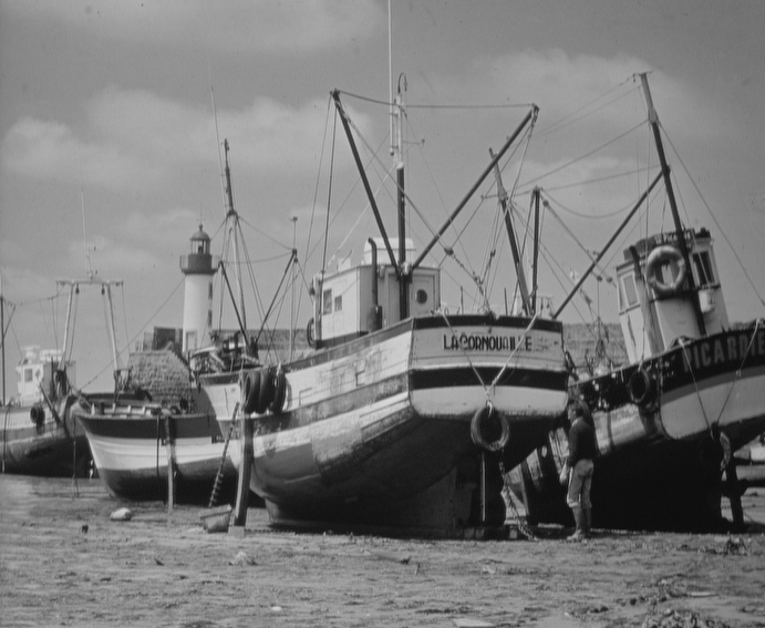
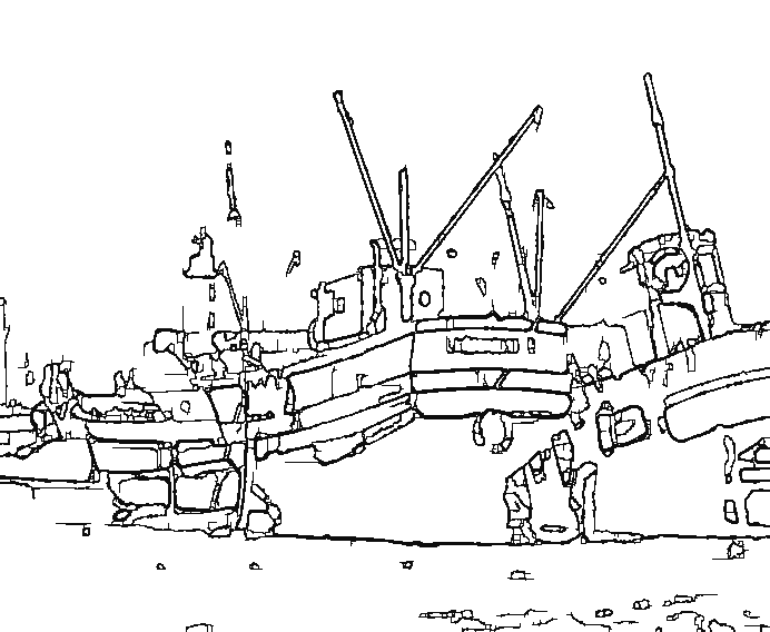
Fig. 1: Upper left: Original image. Upper right: Smoothing with the Ambrosio–Tortorelli Approximation. Middle left: Smoothing with Algorithm 4.1. Middle right: Edge indicator for the Ambrosio–Tortorelli Approximation. Lower left: Edge indicator for Algorithm 4.1. Lower right: Edge indicator for the Ambrosio–Tortorelli Approximation, thresholded at 0.8. For both methods, $\alpha=20$, $\beta=200$, $\varepsilon=0.05$.

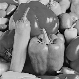
Fig. 2: Upper left: Original image. Upper right: Smoothing with the Ambrosio–Tortorelli Approximation. Middle left: Smoothing with Algorithm 4.1. Middle right: Edge indicator for the Ambrosio–Tortorelli Approximation. Lower left: Edge indicator for Algorithm 4.1. Lower right: Edge indicator for the Ambrosio–Tortorelli Approximation, thresholded at 0.9. For both methods, $\alpha=1$, $\beta=500$, $\varepsilon=0.05$.

5 Conclusion

The results of this paper provide a theoretical connection between the Mumford–Shah functional and techniques from topological asymptotic analysis that have recently been applied to imaging problems like edge detection. We have shown that the Mumford–Shah functional can be approximated, in the sense of $\Gamma$-limits, by a family of set functions that count the number of balls that are necessary to cover the edge set of an image. The placement of these balls can then be determined by an asymptotic expansion of this set function with respect to the radii of the balls.

Apart from providing yet another method for image smoothing and segmentation, our results indicate that all the proposed algorithms using topological asymptotic analysis are somehow related to a classical variational method by means of $\Gamma$-convergence. For the method based on the function $J_{\varepsilon,\kappa}$ defined in (1.3), the relation has been proven explicitly, but similar relations are expected to hold for other methods. For instance, the algorithm proposed in [9] for image segmentation should rightly be regarded as an implementation of the Chan–Vese model [20] without making use of level set methods.

References

• [1] R. A. Adams. Sobolev Spaces. Academic Press, New York, 1975.
• [2] L. Ambrosio. Existence theory for a new class of variational problems. Arch. Ration. Mech. Anal., 111:291–322, 1990.
• [3] L. Ambrosio and V. M. Tortorelli. Approximation of functionals depending on jumps by elliptic functionals via $\Gamma$-convergence. Comm. Pure Appl. Math., 43(8):999–1036, 1990.
• [4] H. Ammari and H. Kang Reconstruction of small inhomogeneities from boundary measurements, volume 1846 of Lecture Notes in Mathematics. Springer, 2004.
• [5] S. Amstutz. Sensitivity analysis with respect to a local perturbation of the material property. Asymptotic Anal., 49(1-2):87–108, 2006.
• [6] G. Aubert, L. Blanc-Féraud, and R. March. An approximation of the Mumford-Shah energy by a family of discrete edge-preserving functionals. Nonlinear Anal., 64(9):1908–1930, 2006.
• [7] G. Aubert and P. Kornprobst. Mathematical Problems in Image Processing: Partial Differential Equations and the Calculus of Variations (second edition), volume 147 of Applied Mathematical Sciences. Springer-Verlag, 2006.
• [8] D. Auroux, L. J. Belaid, and M. Masmoudi. A topological asymptotic analysis for the regularized grey-level image classification problem. Math. Model. Numer. Anal., 41(3), 2007.
• [9] D. Auroux and M. Masmoudi. Image processing by topological asymptotic expansion. J. Math. Imaging Vision, 33(2), 2009.
• [10] A. Blake and A. Zisserman. Visual Reconstruction, MIT Press, 1987.
• [11] A. Braides. Approximation of free-discontinuity problems, volume 1694 of Lecture Notes in Mathematics. Springer-Verlag, Berlin, 1998.
• [12] A. Braides. $\Gamma$-convergence for beginners, volume 22 of Oxford Lecture Series in Mathematics and its Applications. Oxford University Press, Oxford, 2002.
• [13] A. Braides, A. Chambolle, and M. Solci. A relaxation result for energies defined on pairs set-function and applications. ESAIM Control Optim. Calc. Var., 13(4):717–734 (electronic), 2007.
• [14] A. Braides and G. Dal Maso. Non-local approximation of the Mumford-Shah functional. Calc. Var. Partial Differential Equations, 5:293–322, 1997.
• [15] D.J. Cedio-Fengya, S. Moskow and M.S. Vogelius. Identification of conductivity imperfections of small diameter by boundary measurements. Continuous dependence and computational reconstruction. Inverse Problems, 14(3):553–595, 1998.
• [16] A. Chambolle. Mathematical problems in image processing. ICTP Lecture Notes, II. Abdus Salam International Centre for Theoretical Physics, Trieste, 2000. Inverse problems in image processing and image segmentation: some mathematical and numerical aspects, Available electronically at http://www.ictp.trieste.it/~pub_off/lectures/vol2.html.
• [17] A. Chambolle. Image segmentation by variational methods: Mumford-Shah functional and the discrete approximations. SIAM J. Appl. Math., 55(3):827–863, 1995.
• [18] A. Chambolle. Finite-differences discretizations of the Mumford-Shah functional. M2AN Math. Model. Numer. Anal., 33(2):261–288, 1999.
• [19] A. Chambolle and G. Dal Maso. Discrete approximation of the Mumford-Shah functional in dimension two. M2AN Math. Model. Numer. Anal., 33(4):651–672, 1999.
• [20] T. Chan and L. Vese. Active contours without edges. IEEE Trans. Image Process., 10(2):266–277, 2001.
• [21] D. Colton and R. Kress. Integral Equation Methods in Scattering Theory. Wiley, New York, 1983.
• [22] D. Colton and R. Kress. Inverse Acoustic and Electromagnetic Scattering Theory. Springer, 1998.
• [23] G. Cortesani. Strong approximation of GSBV functions by piecewise smooth functions. Ann. Univ. Ferrara Sez. VII (N.S.), 43:27–49 (1998), 1997.
• [24] G. Cortesani and R. Toader. A density result in SBV with respect to non-isotropic energies. Nonlinear Anal., 38(5, Ser. B: Real World Appl.):585–604, 1999.
• [25] G. Dal Maso. An Introduction to $\Gamma$-Convergence, volume 8 of Progress in Nonlinear Differential Equations and their Applications. Birkhäuser, 1993.
• [26] G. Dal Maso, J. M. Morel, and S. Solimini. A variational method in image segmentation: Existence and approximation results. Acta Mathematica, 168(1):89–151, 1992.
• [27] E. De Giorgi, M. Carriero, and A. Leaci. Existence theorem for a minimum problem with free discontinuity set. Arch. Ration. Mech. Anal., 108:195–218, 1989.
• [28] L. C. Evans. Partial Differential Equations, 2nd Edition. AMS Press, 2010.
• [29] R. A. Feijóo, A. Novotny, C. Padra, and E. Taroco. The topological derivative for the Poisson problem. Math. Mod. Meth. Appl. Sci., 13(12):1825–1844, 2003.
• [30] S. Garreau, P. Guillaume, and M. Masmoudi. The topological asymptotic for PDE systems: The elasticity case. SIAM J. Control Optimiz, 39(6):1756–1778, 2000.
• [31] D. Gilbarg and N. Trudinger. Elliptic Partial Differential Equations of Second Order. Classics in Mathematics. Springer Verlag, Berlin, 2001. Reprint of the 1998 edition.
• [32] S. M. Giusti, A. A. Novotny, C. Padra. Topological sensitivity analysis of inclusion in two-dimensional linear elasticity. Engineering Analysis with Boundary Elements, 32(11):926–935, 2008.
• [33] G. Koepfler, C. Lopez, and J. M. Morel. A multiscale algorithm for image segmentation by variational method. SIAM J. Numer. Anal., 31(1):282–299, 1994.
• [34] S. G. Krein and Yu. I. Petunin. Scales of Banach spaces. Russ. Math. Surv., 21(85):85–159, 1966.
• [35] R. Kress. Linear Integral Equations. Springer, 1989.
• [36] J.-M. Morel and S. Solimini. Variational Methods in Image Segmentation. Birkhäuser, Boston, 1995.
• [37] D. Mumford and J. Shah. Optimal approximations by piecewise smooth functions and associated variational problems. Comm. Pure Appl. Math., 42(5):577–685, 1989.
• [38] M. Muszkieta. Optimal edge detection by topological asymptotic analysis. Math. Mod. Meth. Appl. Sci., 19(11):2127–2143, 2009.
• [39] P. D. Polyanin. Handbook of Linear Partial Differential Equations. Chapman & Hall, 2002.
• [40] O. Scherzer, editor. Handbook of Mathematical Methods in Imaging. Springer-Verlag New York Inc., 2010.
• [41] O. Scherzer, M. Grasmair, H. Grossauer, M. Haltmeier, and F. Lenzen. Variational methods in imaging, volume 167 of Applied Mathematical Sciences. Springer, New York, 2009.
• [42] J. Sokołowski and A. Żochowski. On topological derivative in shape optimization. SIAM J. Control Optimiz, 37(4):1251–1272, 1999.
• [43] J. Spanier. An Atlas of Functions. Taylor & Francis, 1987.
• [44] M. S. Vogelius and D. Volkov. Asymptotic formulas for perturbations in the electromagnetic fields due to the presence of inhomogeneities of small diameter. Math. Model. Numer. Anal., 34(4):723–748, 2000.