Optical response of graphene under intense terahertz fields

Abstract

Optical responses of graphene in the presence of intense circularly and linearly polarized terahertz fields are investigated based on the Floquet theory. We examine the energy spectrum and density of states. It is found that gaps open in the quasi-energy spectrum due to the single-photon/multi-photon resonances. These quasi-energy gaps are pronounced at small momentum, but decrease dramatically with the increase of momentum and finally tend to be closed when the momentum is large enough. Due to the contribution from the states at large momentum, the gaps in the density of states are effectively closed, in contrast to the prediction in the previous work by Oka and Aoki [Phys. Rev. B 79, 081406(R) (2009)]. We also investigate the optical conductivity for different field strengths and Fermi energies, and show the main features of the dynamical Franz-Keldysh effect in graphene. It is discovered that the optical conductivity exhibits a multi-step-like structure due to the sideband-modulated optical transition. It is also shown that dips appear at frequencies being the integer numbers of the applied terahertz field frequency in the case of low Fermi energy, originating from the quasi-energy gaps at small momentums. Moreover, under a circularly polarized terahertz field, we predict peaks in the middle of the “steps” and peaks induced by the contribution from the states around zero momentum in the optical conductivity.

I Introduction

Since the experimental realization of graphene,Novoselov_04 a monolayer of carbon atoms arranged in a honeycomb lattice, this material has aroused enormous interest due to its unique physical characteristics.Geim_rev_nat ; Neto_rev_09 ; Beenakker_rev ; Orlita_rev ; Chakraborty_rev ; Peres_rev ; Mucciolo_rev ; Sarma_rev ; Ferreira_dc Among different works in this field, the linear optical property of graphene is one of the main focuses of attention.Orlita_rev ; Gusynin ; Ando_02 ; Neto_06 ; Stauber_disorder ; Stauber_NN ; Giuliani_ee ; exp_Basov ; exp_Nair ; exp_APL The theoretical works based on the Dirac Hamiltonian show that the optical conductivity at high frequency is dominated by the interband optical conductivity, which takes a constant value of $\sigma_{0}=\frac{e^{2}}{4\hbar}$ for frequency larger than twice of the Fermi energy $E_{F}$ and approaches to zero for frequency below $2E_{F}$ due to the Pauli blocking.Gusynin ; Ando_02 ; Neto_06 ; Stauber_disorder ; Giuliani_ee The universal value $\sigma_{0}$ of optical conductivity has been demonstrated to be valid not only in the noninteracting limit,Ando_02 ; Gusynin but also in the presence of the disorder and the electron-electron interaction as long as the Dirac-cone approximation remains valid.Neto_06 ; Stauber_disorder ; Giuliani_ee The constant optical conductivity in a wide range of frequency also has been observed in the optical experiments.exp_Basov ; exp_Nair ; exp_APL On the other hand, the optical conductivity at low frequency is determined by the intraband optical conductivity, which presents a Drude peak centred at zero frequency and is strongly influenced by the sample-dependent scattering behavior.Gusynin ; Ando_02 ; Neto_06 ; Stauber_disorder

Recently, influence of an intense ac field on electrical and optical properties in graphene has also attracted much attention. Gupta_dis2 ; Naumis_pol ; Syzranov_08 ; Oka_cur ; Zhang_energy ; Fistul_07 ; Kibis_quantiz ; Oka_opt ; Mikhailov_multi ; Wright_09 ; Oka_cur2 ; Ryzhii_dc ; Ryzhii_dcac ; Ryzhii_BG ; Wright_BG ; Abergel_BG ; Abergel_BG2 It has been found that the application of an intense ac field can dramatically modify the band structure and hence the density of states (DOS).Oka_cur ; Oka_cur2 ; Kibis_quantiz ; Zhang_energy ; Naumis_pol ; Syzranov_08 Their results also showed that a stationary energy gap appears around the Dirac point under a circularly polarized ac field.Oka_cur ; Kibis_quantiz Oka and AokiOka_cur ; Oka_cur2 ; Oka_opt calculated the dc and ac conductivities in graphene irradiated by an intense circularly polarized light via the extended Kubo formula, and proposed the photovoltaic Hall effect, which is a novel Hall effect occuring in the absence of uniform magnetic fields. The dc transport properties of graphene-based p-n junctions under an intense ac field were also investigated theoretically.Fistul_07 ; Syzranov_08 However, contribution in the optical spectra in graphene from the optical sidebandsKono_sideband ; Phillips_sideband ; Maslov_sideband ; Nordstrom_exp_EDFK ; Holthaus_Stark ; Rodriguez_Stark ; Yacoby_68 ; Jauho_DFK ; Chin_exp_20 ; Zhang_exp_06 ; Srivastava_exp_DFK has not yet been well investigated.

In semiconductors, the contribution from the sidebands has been demonstrated to be important for the optical and transport properties. Many interesting phenomena, such as the photon-assisted tunneling,Hanggi_98 ; Hanggi_05 the sideband generation of exciton,Kono_sideband ; Phillips_sideband ; Maslov_sideband ; Nordstrom_exp_EDFK the ac Stark effect,Holthaus_Stark ; Nordstrom_exp_EDFK ; Rodriguez_Stark and the dynamical Franz-Keldysh (DFK) effect,Yacoby_68 ; Jauho_DFK ; Chin_exp_20 ; Zhang_exp_06 ; Srivastava_exp_DFK as well as spin generation and manipulation utilized by the intense terahertz (THz) fieldCheng_APL ; Jiang_JAP ; Zhou_PE ; Jiang_PRB_07 ; Jiang_PRB_08 are related to the formation of sidebands. Among these effects, the DFK effect describes the influence on optical spectra from the sidebands of the expanded states,Yacoby_68 ; Jauho_DFK which includes finite absorption below the band edge from the contribution of the sidebands below the bottom of the conduction band and the step-like behavior above the band edge due to the sideband-modulated generalized DOS. Just as the DFK effect in semiconductors, the formation of optical sidebands should also influence the optical spectra near the absorption edge around $2E_{\rm F}$ in graphene. Nevertheless, the band structure of graphene is gapless and the energy dispersion is linear, which is quite distinct from semiconductors. Thus the DFK effect in graphene is expected to present some unique behaviors. This makes the investigation on this problem become very interesting and important. It is also noted that in previous investigationOka_opt only the optical conductivity with $E_{\rm F}$ much smaller than the frequency of the ac field was discussed and thus the contribution from the optical sidebands is difficult to identify. In the present work, we calculate the optical conductivity of graphene under the intense THz field for various Fermi energies and field strengths in order to gain a complete view of the DFK effect in graphene.

In order to include the contribution from the optical sidebands explicitly, we solve the time-dependent Schrödinger equation by using the Floquet theoryShirley_65 and obtain the optical conductivity in graphene under an intense THz field via the nonequlibrium Green functions.Jauho_DFK ; Haug_08 In this paper, we focus on the optical conductivity at high frequency, which is known to be insensitive to the scattering strength.Orlita_rev ; Gusynin ; Ando_02 ; Neto_06 ; Stauber_disorder ; Stauber_NN ; Giuliani_ee ; exp_Basov ; exp_Nair ; exp_APL This allows us to ignore the detail of the scattering and only discuss the optical conductivity in the noninteracting limit. We first examine the energy spectrum and DOS. It is found that gaps appear in the quasi-energy spectrum due to the single-photon/multi-photon resonances.Holthaus_Stark ; Hanggi_98 These quasi-energy gaps are pronounced at small momentum, in consistence with the previous investigations.Oka_cur ; Kibis_quantiz ; Syzranov_08 However, the quasi-energy gaps decrease dramatically with the increase of momentum and finally disappear when the momentum is large enough. Therefore after taking account of the contribution from the states with large momentum, gaps in the DOS are effectively closed, in contrast to the prediction by Oka and Aoki.Oka_cur Our results of the optical conductivity reveal the main features of the DFK effect in graphene.

This paper is organized as follows. In Sec. IIA, we obtain the energy spectrum by exploiting the Floquet theory. Then in Sec. IIB, we derive the optical conductivity via the nonequlibrium Green functions. The numerical results of the DOS and optical conductivity are presented in Sec. III. Finally, we summarize in Sec. IV.

II Model and Formalism

II.1 Hamiltonian

We consider a graphene layer placed in the $x$-$y$ plane. In the vicinity of the Dirac point, the effective Hamiltonian of graphene can be written as ($\hbar\equiv 1$)DiVincenzo

$$\hat{H}_{0}^{\mu}({\bf k}) = v_{\rm F}(\mu\hat{\sigma}_{x}k_{x}+\hat{\sigma}_{y}k_{y}).$$ (1)

Here $\mu=1(-1)$ for $K(K^{\prime})$ valley; $v_{\rm F}$ is the Fermi velocity; ${\bf k}$ represents the two-dimensional wave vector relative to $K(K^{\prime})$ point; $\hat{\bm{\sigma}}$ is the Pauli matrix in the pseudospin space formed by the A and B sublattices of the honeycomb lattice. Here and hereafter, symbols with $\hat{\mbox{}}$ present the $2\times 2$ matrices in the pseudospin space. The eigenvalue and eigenvector of $\hat{H}_{0}^{\mu}$ are $E_{{\bf k}\nu}^{\mu}=\nu v_{\rm F}|{\bf k}|$ and $\zeta_{{\bf k}\nu}^{\mu}=1/\sqrt{2}(\mu\nu e^{-i\mu\theta_{\bf k}},1)^{\rm T}$, respectively, with $\nu$ being 1 $(-1)$ for electron (hole) band and $\theta_{\bf k}$ representing the polar angle of ${\bf k}$. Substituting ${\bf k}$ by ${\bf k}+e{\bf A}(t)$, one obtains the effective Hamiltonian in the presence of a THz field

$$\hat{H}_{\rm eff}^{\mu}({\bf k},t) = \hat{H}_{0}^{\mu}({\bf k})+\hat{H}_{\rm THz}^{\mu}(t),$$ (2)

$$\hat{H}_{\rm THz}^{\mu}(t) = ev_{\rm F}[\mu\hat{\sigma}_{x}A_{x}(t)+\hat{\sigma}_{y}A_{y}(t)].$$ (3)

For convenience, we choose the THz field as ${\bf E}(t)=E_{0}({\bf e}_{x}\cos\theta_{\bf E}\cos\Omega t+{\bf e}_{y}\sin\theta_{\bf E}\sin\Omega t)$. Thus the vector potential ${\bf A}(t)$ reads ${\bf A}(t)=\frac{E_{0}}{\Omega}(-{\bf e}_{x}\cos\theta_{\bf E}\sin\Omega t+{\bf e}_{y}\sin\theta_{\bf E}\cos\Omega t)$. For $\theta_{\bf E}=0$, $\pi/4$ and $\pi/2$, the THz fields are linearly polarized along the $x$-axis, circularly polarized and linearly polarized along the $y$-axis, respectively. Without loss of generality, we set the THz field linearly polarized along the $x$-axis when discussing the case for a linearly polarized THz field.

By exploiting the Floquet theory,Shirley_65 the solution of the Schrödinger equation $i\partial_{t}|\Phi_{{\bf k}\alpha}^{\mu}(t)\rangle=\hat{H}_{\rm eff}^{\mu}({\bf k},t)|\Phi_{{\bf k}\alpha}^{\mu}(t)\rangle$ has the form ( $|\Phi_{{\bf k}\alpha}^{\mu}(t)\rangle$ is referred to as the Floquet state in the following):

$$|\Phi_{{\bf k}\alpha}^{\mu}(t)\rangle=e^{-i\mathcal{E}_{{\bf k}\alpha}^{\mu}t}\sum_{n=-\infty}^{\infty}e^{in\Omega t}|\psi^{n}_{\mu{\bf k}\alpha}\rangle,$$ (4)

in which $\alpha$ represents the branch index of the solution; $\mathcal{E}_{{\bf k}\alpha}^{\mu}$ and $|\psi^{n}_{\mu{\bf k}\alpha}\rangle=(\psi^{n+}_{\mu{\bf k}\alpha},\psi^{n-}_{\mu{\bf k}\alpha})^{\rm T}$ are the eigenvalue (quasi-energy) and eigenvector determined by

$$(\frac{\mathcal{E}_{{\bf k}\alpha}^{\mu}}{\Omega}-n)\psi^{n\sigma}_{\mu{\bf k}\alpha}=\frac{i\beta}{2}[(\mu\cos\theta_{\bf E}-\sigma\sin\theta_{\bf E})\psi^{n-1\,-\sigma}_{\mu{\bf k}\alpha}$$

$$\mbox{}-(\mu\cos\theta_{\bf E}+\sigma\sin\theta_{\bf E})\psi^{n+1\,-\sigma}_{\mu{\bf k}\alpha}]+\frac{v_{\rm F}k}{\Omega}\mu e^{-i\mu\sigma\theta_{\bf k}}\psi^{n\,-\sigma}_{\mu{\bf k}\alpha},$$ (5)

with $\beta={v_{\rm F}eE_{0}}/{\Omega^{2}}$. The above equation shows that the relation between the normalized quasi-energy ${\mathcal{E}_{{\bf k}\alpha}^{\mu}}/{\Omega}$ and the normalized momentum ${v_{\rm F}{\bf k}}/{\Omega}$ is only determined by the dimensionless quantity $\beta$.other_def

Due to the periodicity of $\hat{H}_{\rm eff}^{\mu}({\bf k},t)$, the eigenvalues are also periodic, i.e., if $\mathcal{E}_{{\bf k}\alpha}^{\mu}$ is a solution of Eq. (5), then $\mathcal{E}_{{\bf k}\alpha}^{\mu;l}=\mathcal{E}_{{\bf k}\alpha}^{\mu}+l\Omega$ is also a solution. It is evident that the eigenvectors of $\mathcal{E}_{{\bf k}\alpha}^{\mu;l}$ and $\mathcal{E}_{{\bf k}\alpha}^{\mu}$ satisfy $\psi^{l;n\sigma}_{\mu{\bf k}\alpha}=\psi^{n-l\,\sigma}_{\mu{\bf k}\alpha}$, thus $\mathcal{E}_{{\bf k}\alpha}^{\mu;l}$ and $\mathcal{E}_{{\bf k}\alpha}^{\mu}$ correspond to the same physical solution of the Schrödinger equation. Namely, the quasi-energy is a multi-valued quantity of the Floquet state.Faisal_dis2 Nevertheless, for each momentum and each valley, the number of the independent quasi-energies is 2, which is determined by the dimension of the Hilbert space. For convenience, we choose the independent quasi-energies $\varepsilon_{{\bf k}\eta}^{\mu}$ in the reduced Floquet zone $(-\Omega/2,\Omega/2]$, with $\eta=\pm$ representing the index of independent solutions. These quasi-energies are referred to as the reduced quasi-energies in the following. The corresponding eigenvectors are labelled as $|\phi^{n}_{\mu{\bf k}\eta}\rangle$. Therefore, by choosing the proper integer $l$, arbitrary quasi-energy $\mathcal{E}^{\mu}_{{\bf k}\alpha}$ and the corresponding eigenvectors $\psi^{n\sigma}_{\mu{\bf k}\alpha}$ can be written into the form

$$\mathcal{E}^{\mu}_{{\bf k}\alpha}=\varepsilon^{\mu}_{{\bf k}\eta}+l\Omega,$$ (6)

$$\psi^{n\sigma}_{\mu{\bf k}\alpha}=\phi^{n-l\,\sigma}_{\mu{\bf k}\eta}.$$ (7)

In addition, for the reduced quasi-energies with different $\eta$, one has

$$\varepsilon_{{\bf k}+}^{\mu} = -\varepsilon_{{\bf k}-}^{\mu},$$ (8)

$$|\phi^{n}_{\mu{\bf k}+}\rangle = \sigma_{y}|\phi^{-n}_{\mu{\bf k}-}\rangle^{\ast}.$$ (9)

From Eq. (4), it is seen that the Floquet state $|\Phi_{{\bf k}\eta}^{\mu}(t)\rangle$ (the general solution index $\alpha$ has been replaced by the independent solution index $\eta$) contains Fourier components with different frequencies, quite distinct from the eigenstate of $H_{0}$, which only takes one eigen-frequency. Each Fourier component corresponds to a sideband of this Floquet state. For the Floquet states with reduced quasi-energy $\varepsilon^{\mu}_{{\bf k}\eta}$, sidebands appear at the frequencies (quasi-energies)

$${\xi}_{{\bf k}\eta}^{\mu;n}=\varepsilon_{{\bf k}\eta}^{\mu}-n\Omega$$ (10)

and the corresponding weights are

$$W^{\mu;n}_{{\bf k}\eta}=\langle\phi^{n}_{\mu{\bf k}\eta}|\phi^{n}_{\mu{\bf k}\eta}\rangle.$$ (11)

From Eqs. (8) and (9), one can see that the quasi-energies and weights of the sidebands satisfy

$${\xi}_{{\bf k}+}^{\mu;n} = -{\xi}_{{\bf k}-}^{\mu;m}-(n+m)\Omega,$$ (12)

$$W^{\mu;n}_{{\bf k}+} = W^{\mu;-n}_{{\bf k}-}.$$ (13)

Besides the quasi-energy, another important quantity of the Floquet state is the mean energyGupta_dis2 ; Faisal_dis2 ; Hsu_dis2 ; Martinez_meanenergy

$$\overline{\varepsilon}_{{\bf k}\eta}^{\mu} = \frac{1}{T_{0}}\int^{T_{0}}_{0}dt\langle\Phi_{{\bf k}\eta}^{\mu}(t)|\hat{H}_{\rm eff}^{\mu}|\Phi_{{\bf k}\eta}^{\mu}(t)\rangle$$ (14)

$$= \varepsilon_{{\bf k}\eta}^{\mu}-\sum_{n\sigma}n\Omega{\phi_{\mu{\bf k}\eta}^{n\sigma\ast}}\phi_{\mu{\bf k}\eta}^{n\sigma},$$

where $T_{0}=2\pi/\Omega$ is the period of the applied THz field. Independent of the choice of the quasi-energy, the mean energy is a single-valued structure quantity of the Floquet state. Thus in previous works,Gupta_dis2 ; Faisal_dis2 ; Hsu_dis2 the mean energy was utilized to identify the filled Floquet states, i.e. states with lower mean energy will be occupied at first. In this paper, we also use this ansatz to obtain the distribution function of the Floquet state, which will be discussed in the next subsection. Moreover, the mean energy is used to identify whether the Floquet state is electron- or hole-like. Analogous to the definition of the electron and hole states in the field-free case, we define the quasi-electron ($\eta=+$) and quasi-hole states ($\eta=-$) as the Floquet states satisfying $\overline{\varepsilon}_{{\bf k}+}^{\mu}>0$ and $\overline{\varepsilon}_{{\bf k}-}^{\mu}<0$, respectively.

II.2 Optical conductivity

It is known that the optical absorption is measured by the real part of optical conductivity.Orlita_rev ; Gusynin ; Ando_02 ; Neto_06 ; Stauber_disorder ; Stauber_NN ; Giuliani_ee ; exp_Basov ; exp_Nair ; exp_APL Therefore we focus on the real part of the optical conductivity in the following. For the probing light field of frequency $\omega_{l}$ with the polarization in the $l$ $(=x,y)$ direction, the linear-response theory yields the real part of optical conductivity:

$${\rm Re}\sigma_{ll}(T,\omega_{l})=-\frac{g_{s}g_{v}}{\omega_{l}}{\rm Im}\Pi^{r}_{ll}(T,\omega_{l}).$$ (15)

Here $g_{v}=2$ and $g_{s}=2$ are the valley and spin degeneracies, respectively; $\Pi_{ll}^{r}(T,\omega_{l})$ is retarded current-current correlation function in the $K$ valley. Here and hereafter we only give the correlation function in the $K$ valley and omit the valley index $\mu$ in all symbols, as the contributions to optical conductivity from both valleys are identical. $\Pi_{ll}^{r}(T,\omega_{l})$ can be written as

$$\Pi^{r}_{ll}(T,\omega_{l})=\int_{-\infty}^{\infty}{\rm d}\tau\,e^{i\omega_{l}\tau}\Pi^{r}_{ll}(T+\frac{\tau}{2},T-\frac{\tau}{2}),$$ (16)

where

$$\Pi_{ll}^{r}(t,t^{\prime})=-{i}\theta(t-t^{\prime})\langle[j^{l}(t),j^{l}(t^{\prime})]\rangle$$ (17)

with $j^{l}=ev_{\rm F}\sigma_{l}$ presenting the $l$ component of the current operator in graphene.Ando_02 ; Neto_06 Via the nonequlibrium Green function method,Jauho_DFK ; Haug_08 we have

$$\Pi_{ll}^{r}(t,t^{\prime}) = {-i}\sum_{{\bf k}\sigma_{1}\sigma_{2}\atop\sigma_{1}^{\prime}\sigma_{2}^{\prime}}[j^{l}_{{\bf k}\sigma_{1}\sigma_{2}}G^{r}_{{\bf k}\sigma_{2}\sigma_{1}^{\prime}}(t,t^{\prime})j^{l}_{{\bf k}\sigma_{1}^{\prime}\sigma_{2}^{\prime}}G^{<}_{{\bf k}\sigma_{2}^{\prime}\sigma_{1}}(t^{\prime},t)$$ (18)

$$\mbox{}+j^{l}_{{\bf k}\sigma_{1}\sigma_{2}}G^{<}_{{\bf k}\sigma_{2}\sigma_{1}^{\prime}}(t,t^{\prime})j^{l}_{{\bf k}\sigma_{1}^{\prime}\sigma_{2}^{\prime}}G^{a}_{{\bf k}\sigma_{2}^{\prime}\sigma_{1}}(t^{\prime},t)],$$

with $G^{r(a,<)}_{{\bf k}\sigma_{1}\sigma_{2}}(t,t^{\prime})$ representing the retarded (advanced, lesser) single-particle Green function.Haug_08 Substituting Eq. (18) into Eq. (16), one has

$$\Pi_{ll}^{r}(T,\omega_{l}) = {-i}\sum_{{\bf k}\sigma_{1}\sigma_{2}\atop\sigma_{1}^{\prime}\sigma_{2}^{\prime}}\int_{-\infty}^{\infty}{{\rm d}\omega\over 2\pi}j^{l}_{{\bf k}\sigma_{1}\sigma_{2}}j^{l}_{{\bf k}\sigma_{1}^{\prime}\sigma_{2}^{\prime}}G^{<}_{{\bf k}\sigma_{2}^{\prime}\sigma_{1}}(T,\omega)$$ (19)

$$\mbox{}\times\big{[}G^{r}_{{\bf k}\sigma_{2}\sigma_{1}^{\prime}}(T,\omega+\omega_{l})+G^{a}_{{\bf k}\sigma_{2}\sigma_{1}^{\prime}}(T,\omega-\omega_{l})\big{]}.$$

Since $\left[G_{{\bf k}\sigma_{1}\sigma_{2}}^{<}(t,t^{\prime})\right]^{\ast}=-G_{{\bf k}\sigma_{2}\sigma_{1}}^{<}(t^{\prime},t)$ and $\left[G_{{\bf k}\sigma_{1}\sigma_{2}}^{a}(t,t^{\prime})\right]^{\ast}=G_{{\bf k}\sigma_{2}\sigma_{1}}^{r}(t^{\prime},t)$, $\Pi_{ll}^{r}(t,t^{\prime})$ is real. Thus one obtains

$${\rm Im}\Pi_{ll}^{r}(T,\omega_{l})={1\over 2i}[\Pi_{ll}^{r}(T,\omega_{l})-\Pi_{ll}^{r}(T,-\omega_{l})]$$

$$={i\over 2}\sum_{{\bf k}\sigma_{1}\sigma_{2}\atop\sigma_{1}^{\prime}\sigma_{2}^{\prime}}\int_{-\infty}^{\infty}{{\rm d}\omega\over 2\pi}j^{l}_{{\bf k}\sigma_{1}\sigma_{2}}j^{l}_{{\bf k}\sigma_{1}^{\prime}\sigma_{2}^{\prime}}\big{[}A_{{\bf k}\sigma_{2}\sigma_{1}^{\prime}}(T,\omega+\omega_{l})$$

$$\hskip 9.95863pt\mbox{}-A_{{\bf k}\sigma_{2}\sigma_{1}^{\prime}}(T,\omega-\omega_{l})\big{]}G^{<}_{{\bf k}\sigma_{2}^{\prime}\sigma_{1}}(T,\omega).$$ (20)

In above equations, we have used the relation $A_{{\bf k}\sigma_{1}\sigma_{2}}(T,\omega)=i[G_{{\bf k}\sigma_{1}\sigma_{2}}^{r}(T,\omega)-G_{{\bf k}\sigma_{1}\sigma_{2}}^{a}(T,\omega)]$. In the noninteracting limit, the retarded Green function is given by

$$\hat{G}^{r}_{\bf k}(t_{1},t_{2})=-i\theta(t_{1}-t_{2})\sum_{\eta}|\Phi_{{\bf k}\eta}(t_{1})\rangle\langle\Phi_{{\bf k}\eta}(t_{2})|.$$ (21)

Thus the spectral function in the frequency space can be written as

$$\hat{A}_{{\bf k}}(T,\omega) = \int_{-\infty}^{\infty}{\rm d}\tau\,e^{i\omega\tau}\sum_{\eta}|\Phi_{{\bf k}\eta}(T+\frac{\tau}{2})\rangle\langle\Phi_{{\bf k}\eta}(T-\frac{\tau}{2})|$$ (22)

$$= 2\pi\sum_{nm\eta}e^{i(n-m)\Omega T}|\phi_{{\bf k}\eta}^{n}\rangle\langle\phi_{{\bf k}\eta}^{m}|\delta\big{(}\omega-\varepsilon_{{\bf k}\eta}+(n$$

$$\mbox{}+m)\frac{\Omega}{2}\big{)}.$$

The next step is to calculate $\hat{G}_{\bf k}^{<}(T,\omega)$. The equal-time lesser function can be expressed in the form

$$\hat{G}^{<}_{{\bf k}}(t,t)=i\sum_{\eta_{1}\eta_{2}}\rho_{{\bf k}\eta_{1}\eta_{2}}(t)|\Phi_{{\bf k}\eta_{1}}(t)\rangle\langle\Phi_{{\bf k}\eta_{2}}(t)|.$$ (23)

Here $\rho_{{\bf k}\eta_{1}\eta_{2}}(t)$ is the nonequilibrium density matrix in the Floquet picture,Jiang_PRB_08 ; Kohler_PRE which can be determined by the kinetic equation including the electron-impurity, electron-phonon and electron-electron scatterings.Haug_08 ; Jiang_PRB_08 ; Kohler_PRE ; Wu_rev This approach is very complicated and left as the subject of our future work. Here we obtain the lesser function based on a simple ansatz following the previous works:Gupta_dis2 ; Faisal_dis2 ; Hsu_dis2 the steady-state density matrix is diagonal with the diagonal term $f_{{\bf k}\eta}$ being the Fermi distribution on the mean energy of the Floquet state,

$$\rho_{{\bf k}\eta_{1}\eta_{2}}(t)=f_{{\bf k}\eta}\delta_{\eta_{1}\eta_{2}}=n_{\rm F}(\overline{\varepsilon}_{{\bf k}\eta})\delta_{\eta_{1}\eta_{2}}.$$ (24)

In the present paper, we focus on the case at zero temperature, and then

$$f_{{\bf k}\eta}=\theta(\overline{\varepsilon}_{{\bf k}\eta}-E_{\rm F}),$$ (25)

where the Fermi energy $E_{\rm F}$ can be obtained from

$$N_{e}=g_{s}g_{v}\sum_{{\bf k}\eta}\theta(E_{\rm F}-\overline{\varepsilon}_{{\bf k}\eta}).$$ (26)

Substituting Eq. (24) into Eq. (23), one gets

$$\hat{G}^{<}_{{\bf k}}(t,t)=i\sum_{\eta}f_{{\bf k}\eta}|\Phi_{{\bf k}\eta}(t)\rangle\langle\Phi_{{\bf k}\eta}(t)|.$$ (27)

By further exploiting the generalized Kadanoff-Baym Ansatz,Haug_08 the two-time lesser function can be obtained as

$$\hat{G}^{<}_{{\bf k}}(t,t^{\prime}) = i\hat{G}^{r}_{{\bf k}}(t,t^{\prime})\hat{G}^{<}_{{\bf k}}(t^{\prime},t^{\prime})-i\hat{G}^{<}_{{\bf k}}(t,t)\hat{G}^{a}_{{\bf k}}(t,t^{\prime})$$ (28)

$$= i\sum_{\eta}f_{{\bf k}\eta}|\Phi_{{\bf k}\eta}(t)\rangle\langle\Phi_{{\bf k}\eta}(t^{\prime})|.$$

Then we have

$$\hat{G}^{<}_{{\bf k}}(T,\omega_{l})=i\sum_{\eta}f_{{\bf k}\eta}\hat{A}_{{\bf k}\eta}(T,\omega),$$ (29)

with $\hat{A}_{{\bf k}\eta}(T,\omega)=\int_{-\infty}^{\infty}{\rm d}\tau\,e^{i\omega\tau}|\Phi_{{\bf k}\eta}(T+\frac{\tau}{2})\rangle\langle\Phi_{{\bf k}\eta}(T-\frac{\tau}{2})|$. Using the above equations, one obtains the optical conductivity

$${\rm Re}\sigma_{ll}(T,\omega_{l}) = \frac{g_{s}g_{v}\pi}{\omega_{l}}\sum_{{\bf k}\eta_{1}\eta_{2}n_{1}\atop m_{1}n_{2}m_{2}}\langle\phi_{{\bf k}\eta_{2}}^{m_{2}}|\hat{j}^{l}_{{\bf k}}|\phi_{{\bf k}\eta_{1}}^{n_{1}}\rangle\langle\phi_{{\bf k}\eta_{1}}^{m_{1}}|\hat{j}^{l}_{{\bf k}}|\phi_{{\bf k}\eta_{2}}^{n_{2}}\rangle$$ (30)

$$\mbox{}\times(f_{{\bf k}\eta_{1}}-f_{{\bf k}\eta_{2}}){\rm e}^{i(n_{1}-m_{1}+n_{2}-m_{2})\Omega T}\delta(\varepsilon_{{\bf k}\eta_{1}}$$

$$\mbox{}-\varepsilon_{{\bf k}\eta_{2}}-(n_{1}+m_{1}-n_{2}-m_{2})\frac{\Omega}{2}+w_{l}).$$

The time-averaged optical conductivity can be written as

$${\rm Re}{\sigma}^{\rm ave}_{ll}(\omega_{l})=\frac{1}{T_{0}}\int_{0}^{T_{0}}dT\;{\rm Re}\sigma_{ll}(T,\omega_{l})$$

$$=\frac{g_{s}g_{v}\pi}{\omega_{l}}\sum_{{\bf k}\eta_{1}\eta_{2}\atop Nn_{1}m_{1}}\langle\phi_{{\bf k}\eta_{2}}^{n_{1}-N}|\hat{j}^{l}_{{\bf k}}|\phi_{{\bf k}\eta_{1}}^{n_{1}}\rangle\langle\phi_{{\bf k}\eta_{1}}^{m_{1}}|\hat{j}^{l}_{{\bf k}}|\phi_{{\bf k}\eta_{2}}^{m_{1}-N}\rangle$$

$$\hskip 9.95863pt\mbox{}\times(f_{{\bf k}\eta_{1}}-f_{{\bf k}\eta_{2}})\delta(\varepsilon_{{\bf k}\eta_{1}}-\varepsilon_{{\bf k}\eta_{2}}-N{\Omega}+w_{l}).$$ (31)

It is found that the time-averaged optical conductivity from the nonequlibrium Green functions agrees with that from the extended Kubo formula used in Ref. Oka_opt, (see also Appendix A). However, it is noted that our method not only gives the time-averaged optical conductivity but also the time-dependent one, and thus can provide the dynamical information of optical response, which can be observed via the time-resolved measurements. It is also noted the distribution used by Oka and Aoki,Oka_opt i.e., $f_{{\bf k}\eta}^{\rm ini}=\sum\limits_{\nu l}n_{\rm F}(E_{{\bf k}\nu})|\langle\zeta_{{\bf k}\nu}|\phi_{{\bf k}\eta}^{l}\rangle|^{2}$, is obtained by projecting the equilibrium Fermi distribution in the field-free case to the basis set formed by the Floquet eigenvectors, corresponding to the “sudden approximation”. Obviously, this distribution, referred to as the projected distribution in the following, is quite different from the mean-energy-determined distribution used in this paper. The comparison of the optical conductivities obtained from these two distributions will be addressed in next section.

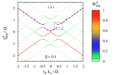
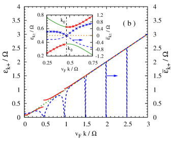
Figure 1: (Color online) Circularly polarized THz field with $\beta=0.4$. (a) Quasi-energies ${\xi}_{{\bf k}\eta}^{n}$ against the normalized momentum. The color coding represents the weight $W_{{\bf k}\eta}^{n}$ of the corresponding sideband. The blue crosses represent the selected quasi-energies of the quasi-electron states. (b) Quasi-energy ${\varepsilon}_{{\bf k}+}$ (red solid curve) and mean energy $\overline{\varepsilon}_{{\bf k}+}$ (blue dashed curve) of the quasi-electron state as well as the field-free electron energy (green dotted curve) against the normalized momentum. In the inset of (b), we plot the quasi-energy around the gap at $k=0.5\Omega/v_{\rm F}$ and ${\varepsilon}_{{\bf k}\eta}=0.5\Omega$ [the region labelled by the box in (a)] as well as the corresponding mean energy as function of momentum. The solid (dashed) curves with and without crosses represent the quasi-energies (mean energies) of the quasi-electron ($\eta=+$) and quasi-hole ($\eta=-$) states, respectively. The black chain line indicates the momentum of the crossover point $k_{0}$. Note the scale of mean energy is on the right-hand side of the frame.

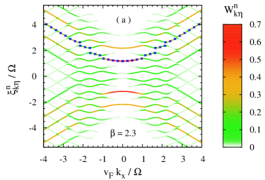
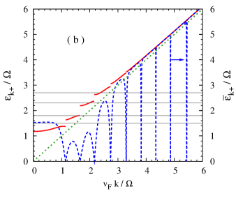
Figure 2: (Color online) Circularly polarized THz field with $\beta=2.3$. (a) Quasi-energies ${\xi}_{{\bf k}\eta}^{n}$ against the normalized momentum. The color coding represents the weight $W_{{\bf k}\eta}^{n}$ of the corresponding sideband. The blue crosses represent the selected quasi-energies of the quasi-electron states. (b) Quasi-energy ${\varepsilon}_{{\bf k}+}$ (red solid curve) and mean energy $\overline{\varepsilon}_{{\bf k}+}$ (blue dashed curve) of the quasi-electron state as well as the field-free electron energy (green dotted curve) versus the normalized momentum. The thin black lines mark the mean energies being $1.5\Omega$, $1.8\Omega$, $2.3\Omega$ and $2.7\Omega$, which are used in the Fig. 6(c). Note the scale of mean energy is on the right-hand side of the frame.

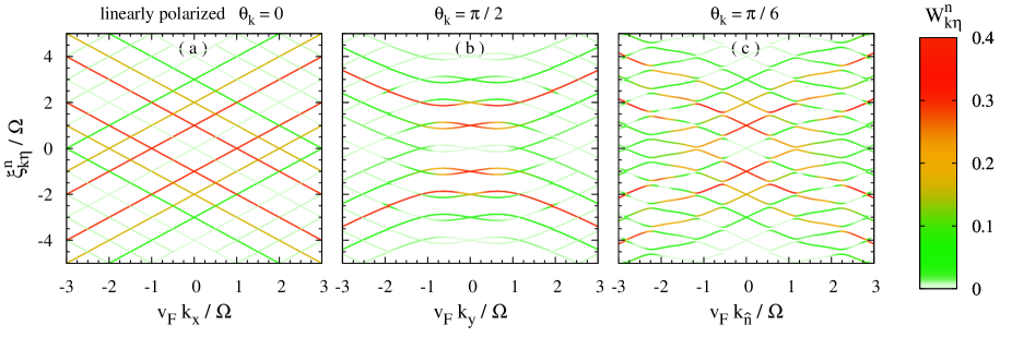
Figure 3: (Color online) Linearly polarized THz field with $\beta=2.3$. Quasi-energies ${\xi}_{{\bf k}\eta}^{n}$ against the normalized momentum for different polar angles $\theta_{\bf k}$. The color coding represents the weight $W_{{\bf k}\eta}^{n}$ of the corresponding sideband. $k_{\hat{\bf n}}$ in (c) stands for ${\bf k}\cdot{\hat{\bf n}}$ with $\hat{\bf n}$ being the unit vector at an angle $\pi/6$ with respect to the $x$-axis.

III Numerical Results

In this section, we discuss the numerical results of the energy spectrum, DOS and optical conductivity of graphene under an intense THz field. The typical parameters used in the computation are $\Omega=5$ THz, $E_{0}=15$ kV$/$cm (corresponding to $\beta=2.3$), $N_{e}=1.5\times 10^{12}$ cm^-2 ($E_{\rm F}=6\Omega$) and $2.5\times 10^{11}$ cm^-2 ($E_{\rm F}=2.7\Omega$). It is noted that our results can be generalized to the other $\Omega$ regime as long as Eq. (24) remains valid, since the behaviors of the energy spectrum and the DOS are only determined by $\beta$ and the behavior of the optical conductivity is only determined by $\beta$ and $E_{\rm F}/\Omega$.gamma We also restrict our investigation of optical conductivity in the frequency regime $\omega_{l}>\Omega$, since the scattering process is not considered in our model and the optical conductivity at low frequency is known to be strongly dependent on the scattering strength.Orlita_rev ; Gusynin ; Ando_02 ; Neto_06 ; Stauber_disorder ; Stauber_NN ; Giuliani_ee ; exp_Basov ; exp_Nair ; exp_APL

III.1 Energy spectrum

Although the energy spectrum in this system has been investigated by many works,Oka_cur ; Oka_cur2 ; Kibis_quantiz ; Zhang_energy ; Naumis_pol ; Syzranov_08 a complete investigation on this problem is still lacking. In particular, the energy spectrum at large momentum has not been well investigated in previous works. In this section, we investigate the energy spectrum under a circularly polarized THz field in a wide range of momentum. Pronounced quasi-energy gaps appear at small momentum in both cases with low and high field strengths. We also discuss the case with a linearly polarized THz field and show that the energy spectrum becomes anisotropic.

We first concentrate on the case for a circularly polarized THz field with low field strength (small $\beta$). In Fig. 1(a), the quasi-energies of the sidebands ${\xi}_{{\bf k}\eta}^{n}$ [Eq. (10)] for $\beta=0.4$ are plotted as function of momentum. Here the color coding represents the weight $W_{{\bf k}\eta}^{n}$ [Eq. (11)] of the corresponding sideband. Since the quasi-energy spectrum is isotropic under a circularly polarized field, we only present the results with $\theta_{\bf k}=0$. The most interesting feature seen in this figure is the appearance of gaps at small momentum in the quasi-energy spectrum, in consistence with the previous investigations.Oka_cur ; Kibis_quantiz ; Syzranov_08 These gaps appear around the momentums $m\Omega/2v_{\rm F}$ and the quasi-energies $m\Omega/2+l\Omega$, with $m$ and $l$ being integers. All gaps at the same momentum share the identical magnitude due to the periodicity of the quasi-energy spectrum. These quasi-energy gaps can be attributed to the ac Stark splittings induced by the single-photon/multi-photon resonances.Holthaus_Stark ; Hanggi_98 ; Faisal_dis2 ; Hsu_dis2 ; Martinez_meanenergy The physics is that if a pair of states are coupled by an electromagnetic field with frequency $\Omega$ and the energy difference between these two states equals to $m\Omega$, then an ac Stark splitting appears unless the corresponding transition is forbidden. Specifically, in the present case, the gaps around the momentum satisfying $2v_{\rm F}k=m\Omega$ are induced by the $m$-photon resonances.gap_zerok

Nevertheless, the behaviour of the quasi-energy spectrum in large momentum regime becomes very different. From Fig. 1(a), one can see that the energy gaps decrease dramatically with the increase of $k$ and finally tend to be closed when the momentum is large enough. This effect can be understood via Eq. (61) under the rotating-wave approximation (the derivation is presented in Appendix B), which shows that the quasi-energy gap around the momentum $m\Omega/2v_{\rm F}$ is determined by the effective coupling parameter $|y_{m}(\theta_{\bf k})|$, given by [see also Eq. (B)]

$$|y_{m}(\theta_{\bf k})|=\frac{1}{\sqrt{2}}|J_{m+1}(\sqrt{2}\beta)-J_{m-1}(\sqrt{2}\beta)|,$$ (32)

with $J_{m}(\sqrt{2}\beta)$ being the Bessel function. Due to the $m$-dependence of $J_{m}(\sqrt{2}\beta)$, the effective coupling parameter $|y_{m}(\theta_{\bf k})|$ decreases dramatically with the increase of $m$ when $m$ is large enough. Thus the quasi-energy gaps become negligible at large momentum. Our calculations also show that, associated with the absence of the gaps, the band-mixing, i.e., the hole (electron) component of the quasi-electron (quasi-hole) state, becomes negligible, and the wave function becomes very close to the one without the interband term of $H_{\rm THz}$.

In Fig. 1(b), we plot the mean energy $\overline{\varepsilon}_{{\bf k}+}$ [Eq. (14)] and the quasi-energy ${\varepsilon}_{{\bf k}+}$ of the quasi-electron state ($\overline{\varepsilon}_{{\bf k}+}>0$) as well as the field-free electron energy for $\beta=0.4$ as function of momentum. In order to compare the above three energies directly, we choose the quasi-energy ${\varepsilon}_{{\bf k}+}$ according to the following rules: 1) the continuity of the quasi-energy is kept as far as possible; 2) the quasi-energy at large momentum is closest to the field-free electron energy. We also plot these selected quasi-energy in Fig. 1(a) (blue crosses). From Fig. 1(b), it is shown that the mean energy and the quasi-energy are far away from (very close to) the field-free energy at small (large) momentum, in consistence with the behaviour of the quasi-energy gap. Moreover, it is also seen that the mean energy reaches zero at a momentum somewhere inside the quasi-energy gap, except the one at zero momentum. In order to reveal the underlying physics, we plot the quasi-energy around the gap at $k=0.5\Omega/v_{\rm F}$ and ${\varepsilon}_{{\bf k}\eta}=0.5\Omega$ [the region labelled by the box in Fig. 1(a)] as well as the corresponding mean energy as function of momentum in the inset of Fig. 1(b). It shows that there is a crossover point (labelled as ${\bf k}_{0}$) between the quasi-hole state (blue solid curve) and the quasi-electron state (red solid curve with crosses) in the quasi-energy above the gap. Since the quasi-energy varies continuously with $k$ at this point, the corresponding mean energy also varies continuously, i.e., $\overline{\varepsilon}_{{\bf k}_{0}+}=\overline{\varepsilon}_{{\bf k}_{0}-}$. Also, from Eqs. (8) and (9), one can see that $\overline{\varepsilon}_{{\bf k}_{0}+}=-\overline{\varepsilon}_{{\bf k}_{0}-}$. Consequently, the mean energies at this point must be zero. The finite mean energy at $k=0$ is based on the similar reason. As shown in Fig. 1(a), the quasi-energy above the gap at zero momentum always belongs to the quasi-electron state [blue crosses in Fig. 1(a)], hence no crossover appears.

Now we turn to the case for a circularly polarized THz field with high field strength (Fig. 2). From Fig. 2(a), it is seen that pronounced quasi-energy gaps appear in a wider range of $k$. However, unlike the previous case, the momentums of the gaps markedly deviate from $m\Omega/(2v_{\rm F})$. This is because the effect of the rapidly varying terms in the resonance equations [Eqs. (52) and (53)] cannot be neglected for strong field, i.e., the rotating-wave approximation is not valid. The joint effect of the terms with different oscillating frequencies leads to the complicated behaviour of the quasi-energy spectrum. However, the quasi-energies where the gaps appear are still around $l\Omega/2$, determined by the symmetry of the quasi-energies of the sidebands [Eq. (13)]. Figure 2 also shows that the quasi-energy gaps become extremely small and the quasi-energy and mean energy become very close to the field-free energy at large momentum. The physics is similar to the weak-field case. When the photon number involved in the resonance becomes too large, the effective resonant coupling becomes extremely weak. Thus the influence of the THz field on the energy spectrum becomes negligible.

Finally we address the case for a linearly polarized THz field (Fig. 3). Here we only present the results with high field strength as they are sufficient for showing the main features in this case. Recall that the linearly polarized THz field is set along the $x$-axis throughout this paper, thus $\theta_{\bf k}$ equals to the angle between the momentum and the THz field. From Fig. 3, it is seen that quasi-energy gaps are closed at zero momentum. This effect can be understood from the exact analytical solution

$$|\Phi_{{\bf k}=0\,\pm}(t)\rangle = \sum_{n}J_{\pm n}(\beta)e^{in\Omega t}(1,\;\pm 1)^{\rm T}.$$ (33)

Clearly, the quasi-energy is zero at zero momentum, thus the gap disappears. Another interesting feature is the anisotropy of the quasi-energy spectrum.Syzranov_08 For momentum along the $x$-axis [Fig. 3(a)], all gaps are closed, since the interband term of ${H}_{\rm THz}$ [Eq. (41)] becomes zero and hence the quasi-energy is exactly the same as the field-free energy, as shown in Eqs. (42) and (43) in Appendix B. For momentum along the $y$-axis [Fig. 3(b)], all gaps except the ones around $k=0.5\Omega/v_{\rm F}$ are effectively closed. This is because the intraband term of ${H}_{\rm THz}$ [Eq. (41)] becomes zero, and thus the gaps from the multi-photon resonances become extremely small, as shown in Fig. 9 in Appendix B. For other polar angle, e.g., $\theta_{\bf k}=\pi/6$ [Fig. 3(c)], pronounced quasi-energy gaps appear not only around $k=0.5\Omega/v_{\rm F}$ but also around the other resonant points at small momentum, similar to the case with a circularly polarized THz field.

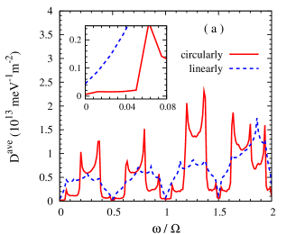
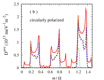
Figure 4: (Color online) (a) Time-averaged DOS versus $\omega$ under circularly (red solid curve) and linearly (blue dashed curve) polarized THz fields for $\beta=2.3$. The region close to $\omega\sim 0$ is enlarged in the inset. (b) Time-averaged DOS versus $\omega$ under a circularly polarized THz field for $\beta=2.3$ with all relevant states (red solid curve), limited in the momentum regimes $v_{\rm F}k<2\Omega$ (blue dashed curve) and $v_{\rm F}k<0.5\Omega$ (green dotted curve). The yellow chain curve represents the DOS from Ref. Oka_cur, .

III.2 DOS

Then we turn to investigate the DOS. By using the spectral function Eq. (22), one obtains the time-averaged DOS

$${D}^{\rm ave}(\omega) = \frac{g_{s}g_{v}}{2\pi T_{0}}\int_{0}^{T_{0}}dT\;\sum_{{\bf k}\eta}{\rm Tr}{A}_{{\bf k}\eta}(T,\omega)$$ (34)

$$= g_{s}g_{v}\sum_{{\bf k}\eta n}\langle\phi_{{\bf k}\eta}^{n}|\phi_{{\bf k}\eta}^{n}\rangle\delta(\omega-\varepsilon_{{\bf k}\eta}+n\Omega)$$

$$= g_{s}g_{v}\sum_{{\bf k}\alpha}\langle\psi_{{\bf k}\alpha}^{0}|\psi_{{\bf k}\alpha}^{0}\rangle\delta(\omega-\mathcal{E}_{{\bf k}\alpha}).$$

The last equality is derived from Eqs. (6) and (7). It is noted that the above equation is in the same form as the one reported by Oka and Aoki.Oka_cur In Fig. 4(a), we plot the time-averaged DOS under circularly and linearly polarized THz fields for $\beta=2.3$. (Note that $\beta=2.3$ corresponds to $F/\Omega=\beta/\sqrt{2}=1.6$ in Ref. Oka_cur, .other_def ) The region close to $\omega\sim 0$ is enlarged in the inset. Here we only show the DOS in the positive frequency regime (electron regime), since the DOS in the negative regime (hole regime) is symmetrical to the positive one.

We first focus on the case for a circularly polarized THz field [red solid curve in Fig. 4(a)]. It is seen that the gaps in the DOS are effectively closed, in contrast to the previous report by Oka and Aoki.Oka_cur The underlying physics is as follows: as shown in Fig. 2(a), the quasi-energy gaps are closed when the momentum is large enough. The contribution from these states closes the gaps in the DOS. We also plot the DOS with all related states (red solid curve), limited in the momentum regimes $v_{\rm F}k<2\Omega$ (blue dashed curve) and $v_{\rm F}k<0.5\Omega$ (green dotted curve) in Fig. 4(b). It is shown that the DOS with $v_{\rm F}k<2\Omega$ (blue dashed curve) is almost the same as the one shown in Ref. Oka_cur, (yellow chain curve). This indicates that the contribution from large momentum is not properly counted in the previous investigation.Oka_cur In addition, it is seen that sharp peaks appear in the DOS. This effect originates from the van Hoff singularities which appear at the momentum of all quasi-energy gaps due to the isotropic quasi-energy spectrum.sing_zerok

Then we turn to the case of a linearly polarized THz field [blue dashed curve in Fig. 4(a)]. It is also shown that the gaps are absent. However the physics is different here. As shown in Fig. 3(a), the quasi-energy gaps disappear for the momentum along the $x$-axis, even at small $k$, and the gaps due to the multi-photon resonances become negligible for momentum along the $y$-axis. Therefore there is no gap in the DOS. Moreover, the peaks from the van Hoff singularities are less pronounced due to the different nature of the van Hoff singularities here associated with anisotropic quasi-energy spectrum.van_Hoff

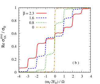
Figure 5: (Color online) Circularly polarized THz field. (a) Time-dependent optical conductivity as function of the optical frequency and time with $\beta=2.3$. (b) Time-averaged optical conductivity as function of the optical frequency with different field strengths. $E_{\rm F}=6\Omega$ in both figures.

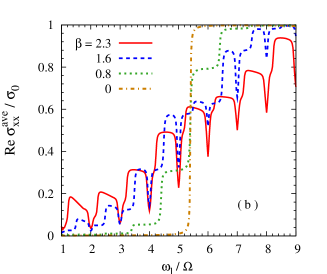
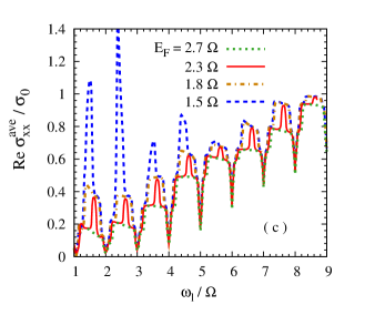
Figure 6: (Color online) Circularly polarized THz field. (a) Time-dependent optical conductivity as function of the optical frequency and time with $\beta=2.3$ and $E_{\rm F}=2.7\Omega$. (b) Time-averaged optical conductivity as function of the optical frequency with different field strengths. $E_{\rm F}=2.7\Omega$. (c) Time-averaged optical conductivity as function of the optical frequency with $\beta=2.3$ for different Fermi energies.

III.3 Optical conductivity

III.3.1 Under a circularly polarized THz field

In this subsection we discuss the optical conductivity under a circularly polarized THz field. Without loss of generality, we restrict ourselves to the $n$-type case, i.e., $E_{\rm F}>0$. Thus only the quasi-electron states with $\overline{\varepsilon}_{{\bf k}\eta}>E_{\rm F}$ are not occupied and the the corresponding interband transitions are allowed.

We first focus on the case with high Fermi energy. The time-dependent and time-averaged optical conductivities as function of the optical frequency $\omega_{l}$ are plotted in Figs. 5(a) and (b), respectively. Here $\sigma_{0}=\frac{e^{2}}{4\hbar}$ is used as the unit of the optical conductivity. It is shown that the optical conductivity exhibits a multi-step-like structure at $\omega_{l}\sim 2E_{\rm F}$, in contrast to the single-step-like behaviour in the field-free case [yellow chain curve in Fig. 5(b)].Orlita_rev ; Gusynin ; Ando_02 ; Neto_06 ; Stauber_disorder ; Stauber_NN ; Giuliani_ee ; exp_Basov ; exp_Nair ; exp_APL Similar to the DFK effect in semiconductors,Jauho_DFK this effect is from the sideband-modulated optical transition, i.e., $n\Omega$ in the delta functions in Eqs. (30) and (31). It is also seen that the number of “step” increases with the increase of the field strength. This can be understood by noticing that the weight of the sideband is distributed in a wider range of frequency for stronger field.

Figure 5 also shows that the optical conductivity varies mildly with the increase of $\omega_{l}$ in each “step”, which is quite different from the DFK effect in semiconductorsJauho_DFK where the optical absorption is strongly dependent on $\omega_{l}$ in each “step”. This behavior can be understood as follows. Since the effect from the interband term of ${H}_{\rm THz}$ becomes negligible at large momentum, the optical conductivity at high Fermi energy can be approximately described by Eq. (66) (the derivation is presented in Appendix C), which indicates that the frequency dependence of the optical conductivity is only from the factor $1-N{\Omega}/{\omega_{l}}$ in the optical transition between the sidebands with the energy difference $2\overline{\epsilon}_{{\bf k}+}+N\Omega$. This factor originates from the linear dispersion of graphene. It is also noted that the optical conductivity is dominated by the optical transitions with small $|N|$, and the pronounced “steps” only appear at $\omega_{l}\sim 2E_{\rm F}$. Thus the frequency dependence of the optical conductivity becomes very weak in each “step” for high Fermi energy.

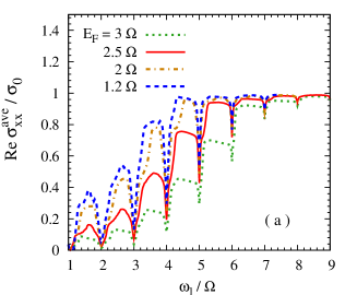
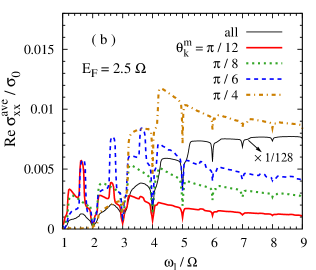
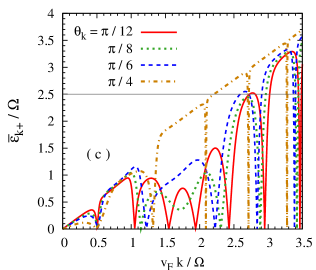
Figure 7: (Color online) Linearly polarized THz field with $\beta=2.3$. (a) Time-averaged optical conductivity as function of the optical frequency for different Fermi energies. (b) Time-averaged optical conductivities versus the optical frequency from the states in different polar angle regions $[\theta^{m}_{\bf k}-\pi/128,\theta^{m}_{\bf k}+\pi/128)$ as well as the one with all polar angles integrated. $E_{\rm F}=2.5\Omega$. (c) Mean energies of the quasi-electron states with different polar angles $\theta_{\bf k}$ against the normalized momentum. The thin black line indicates the mean energy being $2.5\Omega$.

Then we turn to the case with low Fermi energy. The time-dependent and time-averaged optical conductivities are plotted as function of the optical frequency in the cases with $E_{\rm F}=2.7\Omega$ in Figs. 6(a) and (b), respectively. It is seen that dips appear around the frequencies satisfying $l\Omega$ when the applied THz field is strong enough. This is because the states at small momentum, where the quasi-energy gaps become pronounced as shown in Fig. 2(b), can contribute to the optical conductivity in this case. More interesting features are presented in the Fermi energy dependence of optical conductivity [Fig. 6(c)]. It is shown that peaks appear in the middle of the “steps” for $E_{\rm F}=2.3\Omega$ (red solid curve). The scenario is as follows. From Fig. 2(b), it is seen that the maximum of the mean energy $\overline{\varepsilon}_{\bf k+}$ at $2.5\Omega/v_{\rm F}$ is slightly higher than the Fermi energy $2.3\Omega$. Consequently, in this momentum regime only the quasi-electron states around $2.5\Omega/v_{\rm F}$ can contribute to the optical conductivity and hence induces the peaks in the middle of the “steps”. When the Fermi energy decreases, more and more states in this momentum regime can contribute to the optical conductivity. Consequently the peaks become wider and wider, and finally become the new “steps”, as shown in the case with $E_{\rm F}=1.8\Omega$ (yellow chain curve). Moreover, when the Fermi energy decreases to $1.5\Omega$ (blue dashed curve), sharp peaks appear in the optical conductivity. This originates from the contribution around $k=0$, in which $\overline{\varepsilon}_{\bf k+}$ is slightly higher than $1.5\Omega$ as shown in Fig. 2(b). One also notes that the van Hoff singularities at nonzero momentum have no effect on the optical conductivity with finite Fermi energy, since the mean energy is close to zero at the momentum of the quasi-energy gaps, as shown in Fig. 2(b).

III.3.2 Under a linearly polarized THz field

We also plot the time-averaged optical conductivity as function of the optical frequency under a linearly polarized THz field in Fig. 7(a). The behavior in this case is simpler than that under a circularly polarized THz field. The multi-step-like behavior and the dips around $l\Omega$ still appear. Nevertheless, the peaks in the middle of the “steps”, which still appear in the optical conductivity at low frequency for $E_{\rm F}=2.5\Omega$ and $1.2\Omega$, are much less pronounced than the ones under a circularly polarized THz field. In order to reveal the underlying physics, we plot the time-averaged optical conductivity from the states with different polar angles as function of the optical frequency for $E_{\rm F}=2.5\Omega$ in Fig. 7(b). The corresponding mean energies are plotted against the normalized momentum in Fig. 7(c). As mentioned above, the peaks in the middle of the “steps” only appear in the situation satisfying the criteria that a local maximum of the mean energy $\overline{\varepsilon}_{\bf k+}$ is slightly higher than the Fermi energy. From Fig. 7(c), one can see that the above criteria is satisfied for the states with $\theta_{\bf k}=\pi/12$ and $\pi/6$, thus pronounced peaks appear in the optical conductivity from the states with these angles [red solid and blue dashed curves in Fig. 7(b)] and the corresponding angles with the same quasi-energy.angle_symmetry However, this criteria cannot be satisfied for the states with the other polar angles, e.g., $\theta_{\bf k}=\pi/8$ and $\theta_{\bf k}=\pi/4$, so peaks are absent in the corresponding optical conductivity [green dotted and yellow chain curves in Fig. 7(b)]. Therefore, after the summation of the contribution from all polar angles, the peaks in the middle of the “steps” become much less pronounced.

III.3.3 Comparison of the optical conductivities calculated with the mean-energy-determined distribution and the projected distribution

In this subsection, we compare the optical conductivities calculated with the distribution determined by the mean energy and the projected distribution. As mentioned above, the projected distribution used in Ref. Oka_opt, is described by (see also Appendix A)

$$f_{{\bf k}\eta}^{\rm ini}=\sum\limits_{\nu l}n_{\rm F}(E_{{\bf k}\nu})|\langle\zeta_{{\bf k}\nu}|\phi_{{\bf k}\eta}^{l}\rangle|^{2}.$$ (35)

Recall that $E_{{\bf k}\nu}$ and $\zeta_{{\bf k}\nu}$ are the eigenvalue and eigenvector of $\hat{H}_{0}$. From Eq. (35), one can recognize the main features of the projected distribution at zero temperature: at $k<k_{\rm F}=E_{\rm F}/v_{\rm F}$, both the field-free electron and hole states are occupied, thus the corresponding quasi-electron and quasi-hole states are both occupied; at $k>k_{\rm F}$, only the hole state is occupied, so the distribution of the Floquet state is determined by the hole component of this state. Therefore one can see that only the states with $k>k_{\rm F}$ can contribute to the optical conductivity, and the contribution decreases with the increase of the band-mixing.

The time-averaged optical conductivities from the mean-energy-determined distribution and the projected distribution are plotted as function of the optical frequency in Fig. 8. It is seen that in the case with high Fermi energy, the results from both distributions are almost the same. This is because the optical conductivity in this situation is determined by the contribution from the states at large momentum, where the band-mixing is negligible due to the marginal effective resonant coupling. Consequently these two optical conductivities are very close to the approximate formula Eq. (66) in Appendix C. However, at low Fermi energy, it is seen that although the dips due to the quasi-energy gaps also appear in the optical conductivity from the projected distribution, the peaks in the middle of the “steps” and the peaks from the states around zero momentum are absent. The absence of both effects is because the quasi-electron states with small $k$ are occupied in the projected distribution. Thus the corresponding optical transitions are blocked. In addition, it is also shown that the van Hoff singularities do not affect on the optical conductivity from the projected distribution, since the contribution from the states around the momentum of the quasi-energy gaps is extremely small due to the strong band-mixing.

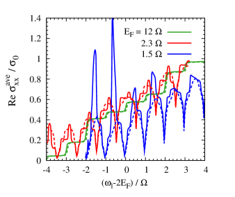
Figure 8: (Color online) Time-averaged optical conductivities from the mean-energy-determined distribution (solid curves) and the projected distribution (dashed curves) are plotted as function of the optical frequency under a circularly polarized THz field with $\beta=2.3$ for different Fermi energies.

IV Summary and discussion

In summary, we have performed a theoretical investigation on the optical responses of graphene in the presence of intense circularly and linearly polarized THz fields via the Floquet theory. We examine the energy spectrum and DOS. It is found that gaps appear at small momentum in the quasi-energy spectrum, in consistence with the previous investigations.Oka_cur ; Kibis_quantiz ; Syzranov_08 These gaps can be attributed to the ac Stark splittings induced by the single-photon/multi-photon resonances. Nevertheless, in large momentum regime, where the energy spectrum has not been well investigated in previous works, we find that the quasi-energy gaps decrease dramatically with the increase of momentum and finally tend to be closed when the momentum is large enough. Consequently, taking account of the contribution from the states at large momentum, the gaps in the DOS are effectively closed, in contrast to the prediction by Oka and Aoki.Oka_cur

We also investigate the optical conductivity from the mean-energy-determined distribution for different field strengths and Fermi energies. These results reveal the main features of the DFK effect in graphene. In the case with high Fermi energy, we discover that the optical conductivity presents a multi-step-like behavior around the optical frequency $\omega_{l}$ twice of the Fermi energy $E_{F}$, in contrast to the single-step-like behaviour in the field-free case. This effect is from the sideband-modulated optical transition, similar to the DFK effect in semiconductors. We also find that the optical conductivity varies mildly with the increase of $\omega_{l}$ in each “step”, which is quite different from the DFK effect in semiconductors. This behaviour is due to the linear dispersion of graphene and the absence of the band-mixing at large momentum.

The behaviour of the optical conductivity becomes more interesting in the case with low Fermi energy. We discover that dips appear at frequencies being the integer numbers of the applied THz field frequency $\Omega$, due to the quasi-energy gaps at small momentums. In the case with a circularly polarized THz field, it is found that peaks appear in the middle of the “steps” when the Fermi energy is slightly lower than a local maximum of the mean energy. This kind of peaks become much less pronounced in the case with a linearly polarized field, owing to the anisotropic energy spectrum. Another interesting finding in the case with a circularly polarized field is that the contribution from the states around zero momentum can induce sharp peaks in the optical conductivity when the Fermi energy is lower than the mean energy at $k=0$.

Finally, we address the distribution function of the Floquet states. Our calculations are based on the ansatz that the distribution function of the Floquet states is determined by the mean energy, following the works in the literature.Gupta_dis2 ; Faisal_dis2 ; Hsu_dis2 The projected distribution function is also adopted in the literature.Oka_opt It is noted that the multi-step-like behavior and the dips around frequencies $l\Omega$ exist in optical conductivities from both distributions. This indicates that these two effects do not depend on the details of the distribution function and thus are expected to be observed in the optical absorption measurements subject to intense THz fields. Nevertheless, the peaks in the middle of the “steps” and the peaks from the states around zero momentum appear only in the optical conductivity from the mean-energy-determined distribution. By performing experimental investigation on these peaks in the optical conductivity, one can distinguish which distribution function of the Floquet state is closest to the genuine one. One may also solve the kinetic equations with all the scattering explicitly includedWu_rev to determine the distribution function.

Appendix A Optical conductivity from extend Kubo formula

We write Eq. (3) in Ref. Oka_opt, into the form

$${\rm Re}{\sigma}^{\rm ave}_{xx}(\omega_{l}) = \frac{4\pi}{\omega_{l}}\sum_{{\bf k}\alpha\beta\atop nm}\langle\psi_{{\bf k}\alpha}^{n}|\hat{j}^{x}_{{\bf k}}|\psi_{{\bf k}\beta}^{n}\rangle\langle\psi_{{\bf k}\beta}^{m}|\hat{j}^{x}_{{\bf k}}|\psi_{{\bf k}\alpha}^{m}\rangle$$ (36)

$$\mbox{}\times(\tilde{f}_{{\bf k}\alpha}-\tilde{f}_{{\bf k}\beta})\delta(\mathcal{E}_{{\bf k}\alpha}-\mathcal{E}_{{\bf k}\beta}+\omega_{l})$$

with $\tilde{f}_{{\bf k}\alpha}=\sum\limits_{\nu}|\langle\zeta_{{\bf k}\nu}|\psi_{{\bf k}\alpha}^{0}\rangle|^{2}n_{\rm F}(E_{{\bf k}\nu})$. Recall that $E_{{\bf k}\nu}$ and $\zeta_{{\bf k}\nu}$ are the eigenvalues and eigenvectors of $\hat{H}_{0}$. By using Eqs. (6) and (7), one obtains

$${\rm Re}{\sigma}^{\rm ave}_{xx}(\omega_{l})=\frac{4\pi}{\omega_{l}}\sum_{{\bf k}\eta_{1}\eta_{2}\atop Nn_{1}n_{2}}\langle\phi_{{\bf k}\eta_{2}}^{n_{1}-N}|\hat{j}^{x}_{{\bf k}}|\phi_{{\bf k}\eta_{1}}^{n_{1}}\rangle\langle\phi_{{\bf k}\eta_{1}}^{n_{2}}|\hat{j}^{x}_{{\bf k}}|\phi_{{\bf k}\eta_{2}}^{n_{2}-N}\rangle$$

$$\hskip 25.6073pt\mbox{}\times(f_{{\bf k}\eta_{1}}^{\rm ini}-f_{{\bf k}\eta_{2}}^{\rm ini})\delta(\varepsilon_{{\bf k}\eta_{1}}-\varepsilon_{{\bf k}\eta_{2}}-N\Omega+\omega_{l})$$ (37)

with $f_{{\bf k}\eta}^{\rm ini}=\sum\limits_{\nu l}n_{\rm F}(E_{{\bf k}\nu})|\langle\zeta_{{\bf k}\nu}|\phi_{{\bf k}\eta}^{l}\rangle|^{2}$. It is seen that the above equation is in the same form as Eq. (31), but the distribution $f_{{\bf k}\eta}^{\rm ini}$ is quite different from $f_{{\bf k}\eta}=n_{\rm F}(\overline{\varepsilon}_{{\bf k}\eta})$ used in the present paper.

Appendix B Approximate analytical solution of Schrödinger equation

We first transform the effective Hamiltonian into the basis set formed by the eigenvectors of $H_{0}$. Thus the Schrödinger equation can be written as

$$\left[v_{\rm F}k\hat{\sigma}_{z}+\tilde{{H}}_{\rm THz}(t)\right]|\Psi_{{\bf k}\eta}(t)\rangle=i\frac{\partial}{\partial t}|\Psi_{{\bf k}\eta}(t)\rangle.$$ (38)

Here $|\Psi_{{\bf k}\eta}(t)\rangle=\hat{U}_{{\bf k}}^{\dagger}|\Phi_{{\bf k}\eta}(t)\rangle$, with the transformation matrix

$$U_{\bf k}=\frac{1}{\sqrt{2}}\begin{pmatrix}e^{-i\theta_{\bf k}}&-e^{-i\theta_{\bf k}}\\ 1&1\end{pmatrix};$$ (39)

$\tilde{{H}}_{\rm THz}(\theta_{\bf k},t)=\hat{U}_{\bf k}^{\dagger}\hat{{H}}_{\rm THz}(t)\hat{U}_{\bf k}$ can be divided into the intraband $\tilde{{H}}^{\rm intra}_{\rm THz}(\theta_{\bf k},t)$ and interband $\tilde{{H}}^{\rm inter}_{\rm THz}(\theta_{\bf k},t)$ terms, given by

$$\tilde{{H}}^{\rm intra}_{\rm THz}(\theta_{\bf k},t) = \beta\Omega\hat{\sigma}_{z}(-\cos\theta_{\bf E}\cos\theta_{\bf k}\sin\Omega t$$ (40)

$$\mbox{}+\sin\theta_{\bf E}\sin\theta_{\bf k}\cos\Omega t),$$

$$\tilde{{H}}^{\rm inter}_{\rm THz}(\theta_{\bf k},t) = \beta\Omega\hat{\sigma}_{y}(\cos\theta_{\bf E}\sin\theta_{\bf k}\sin\Omega t$$ (41)

$$\mbox{}+\sin\theta_{\bf E}\cos\theta_{\bf k}\cos\Omega t).$$

Then we solve the Schrödinger equation without the interband term $\tilde{{H}}^{\rm inter}_{\rm THz}(\theta_{\bf k},t)$ and obtain

$$|\Psi_{{\bf k}+}^{(0)}(t)\rangle = e^{-iv_{\rm F}kt}u^{(0)}(\theta_{\bf k},t)(1,0)^{\rm T},$$ (42)

$$|\Psi_{{\bf k}-}^{(0)}(t)\rangle = e^{iv_{\rm F}kt}[u^{(0)}(\theta_{\bf k},t)]^{\ast}(0,1)^{\rm T},$$ (43)

with

$$u^{(0)}(\theta_{\bf k},t) = \exp\left\{i\beta\cos\theta_{\rm E}\cos\theta_{\bf k}[1-\cos(\Omega t)]\right.$$ (44)

$$\left.\mbox{}-i\beta\sin\theta_{\rm E}\sin\theta_{\bf k}\sin(\Omega t)\right\}.$$

It is evident that $u^{(0)}(\theta_{\bf k},t)$ is a time-periodic function, thus the quasi-energy of $|\Psi_{{\bf k}\eta}^{(0)}(t)\rangle$ is exactly the same as the field-free energy $\eta v_{\rm F}k$. This indicates that all quasi-energy gaps disappear without $\tilde{{H}}^{\rm inter}_{\rm THz}(\theta_{\bf k},t)$ .

The next step is to write the solution of Eq. (38) into the form

$$|\Psi_{{\bf k}\eta}(t)\rangle=a_{\eta,1}(t)|\Psi_{{\bf k}+}^{(0)}(t)\rangle+a_{\eta,2}(t)|\Psi_{{\bf k}-}^{(0)}(t)\rangle.$$ (45)

Substituting Eq. (45) into Eq. (38), one obtains

$$\partial_{t}a_{\eta,1}(t)=-\frac{1}{2}\beta\Omega a_{\eta,2}(t)\sum_{l}y_{l}^{\ast}(\theta_{\bf k})e^{i(2v_{\rm F}k-l\Omega)t},$$ (46)

$$\partial_{t}a_{\eta,2}(t)=\frac{1}{2}\beta\Omega a_{\eta,1}(t)\sum_{l}y_{l}(\theta_{\bf k})e^{-i(2v_{\rm F}k-l\Omega)t},$$ (47)

where

$$y_{l}(\theta_{\bf k})=u_{l-1}^{(1)}(\theta_{\bf k})(\sin\theta_{\bf E}\cos\theta_{\bf k}-i\cos\theta_{\bf E}\sin\theta_{\bf k})$$

$$\mbox{}+u_{l+1}^{(1)}(\theta_{\bf k})(\sin\theta_{\bf E}\cos\theta_{\bf k}+i\cos\theta_{\bf E}\sin\theta_{\bf k}),$$

$$u_{l}^{(1)}(\theta_{\bf k})=\frac{1}{T_{0}}\int_{0}^{T_{0}}dt\,e^{il\Omega t}[u^{(0)}(\theta_{\bf k},t)]^{2}$$

$$\hskip 11.38092pt= e^{i2\beta\cos\theta_{\bf E}\cos\theta_{\bf k}}J_{l}(2|z(\theta_{\bf k})|)\left[\frac{-z(\theta_{\bf k})}{|z(\theta_{\bf k})|}\right]^{l},$$ (50)

$$z(\theta_{\bf k})=\beta(\sin\theta_{\bf E}\sin\theta_{\bf k}+i\cos\theta_{\bf E}\cos\theta_{\bf k}).$$

In above derivation, we have applied the summation rule of the Bessel functionformula

$$J_{l}(|\mathcal{Z}|)(\frac{\mathcal{Z}^{l}}{|\mathcal{Z}|^{l}})=\sum_{j}e^{ij\theta}J_{j}(y)J_{l-j}(x),$$ (51)

with $\mathcal{Z}=x+e^{i\theta}y$ ($x$ and $y$ are real numbers). Since Eqs. (46) and (47) cannot be solved in analytical closed form, we solve these equations via the rotating-wave approximation, which is widely used in the weak electromagnetic field related problem.Hanggi_98 ; Hanggi_05 Exploiting this approximation, we neglect the rapidly varying terms with $l\neq m$ near the resonant point $2v_{\rm F}k\sim m\Omega$ and obtain

$$\partial_{t}a_{\eta,1}(t) = -\frac{1}{2}\beta\Omega a_{\eta,2}(t)y_{m}^{\ast}(\theta_{\bf k})e^{i\delta_{km}t},$$ (52)

$$\partial_{t}a_{\eta,2}(t) = \frac{1}{2}\beta\Omega a_{\eta,1}(t)y_{m}(\theta_{\bf k})e^{-i\delta_{km}t},$$ (53)

with $\delta_{km}=2v_{\rm F}k-m\Omega$. Comparing the multi-photon resonance equations [Eqs. (52) and (53)] with the well-known single-photon resonance equations in the two-level system [e.g., Eq. (83) in Ref. Hanggi_98, ], one can find that the main difference is the appearance of the coefficient $y_{m}(\theta_{\bf k})$.little_change Thus $|y_{m}(\theta_{\bf k})|$ can be treated as a parameter to describe the magnitude of the effective coupling induced by the $m$-photon resonances.

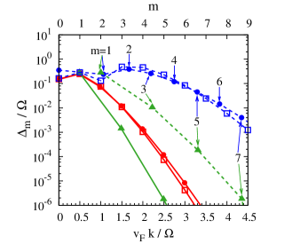
Figure 9: (Color online) Quasi-energy gap $\Delta_{m}$ versus the corresponding momentum from the exact calculation (dots) and the approximate formula Eq. (61) (squares) under circularly polarized THz fields with $\beta=0.4$ (solid curves) and $2.3$ (dashed curves). The triangles represent the results from the exact calculation without the intraband term $\tilde{H}^{\rm intra}_{\rm THz}$. The indices $m$ of the gaps at finite momentum from the exact calculation for $\beta=2.3$ are labelled in the figure. The other gap indices can be read from the $m$-axis on the upper frame. Note that gaps only appear at the momentums where the dots (squares, triangles) indicate. The curves are only plotted as a guide for the eyes.

The solutions of Eqs. (52) and (53) are then easy to obtain:

$$a_{\eta,1}=C_{\eta}^{+}\exp\left\{\frac{it}{2}\left[\delta_{km}-\eta\sqrt{\delta_{km}^{2}+[\Delta^{\prime}_{m}(\theta_{\bf k})]^{2}}\right]\right\},$$ (54)

$$a_{\eta,2}=C_{\eta}^{-}\exp\left\{-\frac{it}{2}\left[\delta_{km}+\eta\sqrt{\delta_{km}^{2}+[\Delta^{\prime}_{m}(\theta_{\bf k})]^{2}}\right]\right\}.$$ (55)

Here

$$\Delta^{\prime}_{m}(\theta_{\bf k})=\beta|y_{m}(\theta_{\bf k})|\Omega;$$ (56)

$C_{\eta}^{+}$ and $C_{\eta}^{-}$ are the normalization coefficients satisfying

$$|C_{\eta}^{+}|^{2}+|C_{\eta}^{-}|^{2}=1,$$ (57)

$$\frac{C_{\eta}^{+}}{C_{\eta}^{-}}=-i\frac{\delta_{km}+\eta\sqrt{\delta_{km}^{2}+[\Delta^{\prime}_{m}(\theta_{\bf k})]^{2}}}{\beta\Omega y_{m}(\theta_{\bf k})}.$$ (58)

Thus one has

$$|\Psi_{{\bf k}\eta}(t)\rangle = e^{-\frac{i}{2}\eta t\sqrt{\delta_{km}^{2}+[\Delta^{\prime}_{m}(\theta_{\bf k})]^{2}}}\Big{(}C_{\eta}^{+}e^{-\frac{i}{2}m\Omega t}u^{(0)}(\theta_{\bf k},t),$$ (59)

$$C_{\eta}^{-}e^{\frac{i}{2}m\Omega t}[u^{(0)}(\theta_{\bf k},t)]^{\ast}\Big{)}^{\rm T}.$$

Evidently, the corresponding quasi-energy is

$$\varepsilon_{{\bf k}\eta}=\frac{\eta}{2}\sqrt{\delta_{km}^{2}+[\Delta^{\prime}_{m}(\theta_{\bf k})]^{2}}.$$ (60)

Thus the quasi-energy gap at the resonant point $\delta_{km}=0$ reads

$$\Delta_{m}(\theta_{\bf k})=\beta|y_{m}(\theta_{\bf k})|\Omega\pmod{\Omega}.$$ (61)

It is seen that the magnitude of the gap $\Delta_{m}(\theta_{\bf k})$ is determined by the effective coupling parameter $|y_{m}(\theta_{\bf k})|$.

In Fig. 9, we plot the magnitude of the quasi-energy gaps $\Delta_{m}$ against the corresponding momentums from the exact calculation (dots) and the approximate formula Eq. (61) (squares) under circularly polarized THz fields with different field strengths. As shown in Figs. 2(a) and (b), the momentums of the gaps from the calculation markedly deviate from $m\Omega/(2v_{\rm F})$ in the strong field regime. Therefore, we define $\Delta_{0}$ as the gap at $k=0$ and $\Delta_{m}$ ($m\neq 0$) as the $m$-th gap from the one at $k=0$ for gaps from the exact calculation. The corresponding indices $m$ are labelled in Fig. 9. In the case with low field strength (red solid curves in Fig. 9), it is seen that the results from the approximate formula agree well with the ones from the exact computation. In the case with high field strength (blue dashed curves), the magnitude of the gaps from these two approaches are comparable, but the corresponding momentums differ significantly, owing to the rotating-wave approximation. In Fig. 9, we also plot the results from the exact calculation without the intraband term $\tilde{H}^{\rm intra}_{\rm THz}$ (triangles). It is seen that except for the gap with $m=1$, the gaps without $\tilde{H}^{\rm intra}_{\rm THz}$ are much smaller than the ones with the intraband term. In particular, the gaps with $m$ being even numbers vanish within the error range of our computation (about $10^{-10}\Omega$). These results indicate that the intraband term $\tilde{H}^{\rm intra}_{\rm THz}$ plays a significant role in the formation of the quasi-energy gaps induced by the multi-photon resonances.

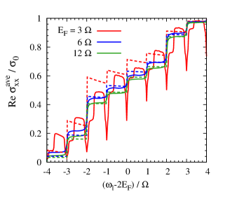
Figure 10: (Color online) Time-averaged optical conductivities from the exact calculation (solid curves) and the the approximate formula Eq. (66) (dashed curves) are plotted as function of the optical frequency under a circularly polarized THz field with $\beta=2.3$ for different Fermi energies.

Appendix C Approximate analytical formula of optical conductivity

Now we discuss the approximate analytical formula of the optical conductivity at high Fermi energy. It is known that the optical conductivity in this case is only from the contribution from the states with large momentum, where the effect from the interband term of ${H}_{\rm THz}$ becomes negligible. Thus one can neglect the interband term and obtain the eigenvector

$$|\Phi_{{\bf k}\eta}(t)\rangle=\hat{U}_{{\bf k}}|\Psi_{{\bf k}\eta}^{(0)}(t)\rangle$$ (62)

in which $U_{\bf k}$ is given by Eq. (39) and $|\Psi_{{\bf k}\eta}^{(0)}(t)\rangle$ is determined by Eqs. (42) and (43). Then one has

$$\overline{\varepsilon}_{{\bf k}\eta} = \varepsilon_{{\bf k}\eta}=\eta v_{\rm F}k,$$ (63)

$$|\phi_{{\bf k}+}^{n}\rangle = u^{(0)}_{n}(\theta_{\bf k})(e^{-i\theta_{\bf k}},1)^{\rm T}/\sqrt{2},$$ (64)

$$|\phi_{{\bf k}-}^{n}\rangle = [u^{(0)}_{-n}(\theta_{\bf k})]^{\ast}(-e^{-i\theta_{\bf k}},1)^{\rm T}/\sqrt{2},$$ (65)

where

$$u^{(0)}_{n}(\theta_{\bf k})=e^{i\beta\cos\theta_{\bf E}\cos\theta_{\bf k}}J_{n}(|z(\theta_{\bf k})|)\left[\frac{-z(\theta_{\bf k})}{|z(\theta_{\bf k})|}\right]^{n}$$

with $z(\theta_{\bf k})$ given by Eq. (50). Substituting Eqs. (63)-(C) into Eq. (31), one obtains

$${\rm Re}{\sigma}^{\rm ave}_{ll}(\omega_{l})=\frac{e^{2}}{4\pi}\sum_{N}(1-N\frac{\Omega}{\omega_{l}})R_{N}\theta({\omega_{l}}-2E_{\rm F}-N{\Omega}),$$

(66)

where

$$R_{N} = \int_{0}^{2\pi}d\theta_{\bf k}\mathcal{A}_{l}^{2}(\theta_{\bf k})J_{N}^{2}(2|z(\theta_{\bf k})|),$$

with $\mathcal{A}_{x}(\theta_{\bf k})=\sin\theta_{\bf k}$ and $\mathcal{A}_{y}(\theta_{\bf k})=\cos\theta_{\bf k}$.

In Fig. 10, we plot the optical conductivities from the exact calculation (solid curves) and the the approximate formula Eq. (66) (dashed curves) as function of the frequency for different Fermi energies. It is seen that the difference between two calculations becomes smaller when the Fermi energy increases. This indicates that the effect from the interband term of ${H}_{\rm THz}$ becomes negligible for high Fermi energy, in consistence with the discussion in the main text.

References

- (1) K. S. Novoselov, A. K. Geim, S. V. Morozov, D. Jiang, Y. Zhang, S. V. Dubonos, I. V. Grigorieva, and A. A. Firsov, Science 306, 666 (2004).
- (2) A. K. Geim and K. S. Novoselov, Nature Mater. 6, 183 (2007).
- (3) A. H. Castro Neto, F. Guinea, N. M. R. Peres, K. S. Novoselov, and A. K. Geim, Rev. Mod. Phys. 81, 109 (2009).
- (4) C. W. J. Beenakker, Rev. Mod. Phys. 80, 1337 (2008).
- (5) D. S. L. Abergel, V. Apalkov, J. Berashevich, K. Ziegler, and T. Chakraborty, Adv. Phys. 59, 261 (2010).
- (6) N. M. R. Peres, Rev. Mod. Phys. 82, 2673 (2010).
- (7) E. R. Mucciolo and C. H. Lewenkopf, J. Phys.: Condens. Matter 22, 273201 (2010).
- (8) S. Das Sarma, S. Adam, E. H. Hwang, and E. Rossi, Rev. Mod. Phys., 2011, in press (also arXiv:1003.4731).
- (9) A. Ferreira, J. Viana-Gomes, J. Nilsson, E. R. Mucciolo, N. M. R. Peres, and A. H. Castro Neto, arXiv:1010.4026.
- (10) M. Orlita and M. Potemski, Semicond. Sci. Technol. 25, 063001 (2010).
- (11) T. Stauber, N. M. R. Peres, and A. K. Geim, Phys. Rev. B 78, 085432 (2008).
- (12) T. Ando, Y. Zheng, and H. Suzuura, J. Phys. Soc. Jpn. 71, 1318 (2002).
- (13) V. P. Gusynin, S. G. Sharapov, and J. P. Carbotte, Phys. Rev. Lett. 96, 256802 (2006).
- (14) N. M. R. Peres, F. Guinea, and A. H. Castro Neto, Phys. Rev. B 73, 125411 (2006).
- (15) T. Stauber, N. M. R. Peres, and A. H. Castro Neto, Phys. Rev. B 78, 085418 (2008).
- (16) A. Giuliani, V. Mastropietro, and M. Porta, arXiv:1101.2169.
- (17) Z. Q. Li, E. A. Henriksen, Z. Jiang, Z. Hao, M. C. Martin, P. Kim, H. L. Stormer, and D. N. Basov, Nat. Phys. 4, 532 (2008).
- (18) R. R. Nair, P. Blake, A. N. Grigorenko, K. S. Novoselov, T. J. Booth, T. Stauber, N. M. R. Peres, and A. K. Geim, Science 320, 1308 (2008).
- (19) J. M. Dawlaty, S. Shivaraman, J. Strait, P. George, M. Chandrashekhar, F. Rana, M. G. Spencer, D. Veksler, and Y. Chen, Appl. Phys. Lett. 93, 131905 (2008).
- (20) S. V. Syzranov, M. V. Fistul, and K. B. Efetov, Phys. Rev. B 78, 045407 (2008).
- (21) T. Oka and H. Aoki, Phys. Rev. B 79, 081406(R) (2009); ibid. 79, 169901(E) (2009).
- (22) T. Oka and H. Aoki, J. Phys.: Conf. Ser. 200, 062017 (2010).
- (23) W. Zhang, P. Zhang, S. Duan, and X. Zhao, New J. Phys. 11, 063032 (2009).
- (24) O. V. Kibis, Phys. Rev. B 81, 165433 (2010).
- (25) F. J. López-Rodríguez and G. G. Naumis, Phys. Rev. B 78, 201406(R) (2008).
- (26) T. Oka and H. Aoki, arXiv:1007.5399.
- (27) M. V. Fistul and K. B. Efetov, Phys. Rev. Lett. 98, 256803 (2007).
- (28) A. K. Gupta, O. E. Alon, and N. Moiseyev, Phys. Rev. B 68, 205101 (2003).
- (29) S. A. Mikhailov and K. Ziegler, J. Phys.: Condens. Matter 20, 384204 (2008).
- (30) A. R. Wright, X. G. Xu, J. C. Cao, and C. Zhang, Appl. Phys. Lett. 95, 072101 (2009).
- (31) F. T. Vasko and V. Ryzhii, Phys. Rev. B 77, 195433 (2008).
- (32) A. Satou, F. T. Vasko, and V. Ryzhii, Phys. Rev. B 78, 115431 (2008).
- (33) V. Ryzhii and M. Ryzhii, Phys. Rev. B 79, 245311 (2009).
- (34) A. R. Wright, J. C. Cao, and C. Zhang, Phys. Rev. Lett. 103, 207401 (2009).
- (35) D. S. L. Abergel and T. Chakraborty, Appl. Phys. Lett. 95, 062107 (2009).
- (36) D. S. L. Abergel and T. Chakraborty, Nanotechnology 22, 015203 (2011).
- (37) J. Černe, J. Kono, T. Inoshita, M. Sherwin, M. Sundaram, and A. C. Gossard, Appl. Phys. Lett. 70, 3543 (1997); J. Kono, M. Y. Su, T. Inoshita, T. Noda, M. S. Sherwin, S. J. Allen, Jr., and H. Sakaki, Phys. Rev. Lett. 79, 1758 (1997).
- (38) K. B. Nordstrom, K. Johnsen, S. J. Allen, A.-P. Jauho, B. Birnir, J. Kono, T. Noda, H. Akiyama, and H. Sakaki, Phys. Rev. Lett. 81, 457 (1998).
- (39) C. Phillips, M. Y. Su, M. S. Sherwin, J. Ko, and L. Coldren, Appl. Phys. Lett. 75, 2728 (1999).
- (40) A. V. Maslov and D. S. Citrin, Phys. Rev. B 62, 16686 (2000).
- (41) M. Holthaus and D. W. Hone, Phys. Rev. B 49, 16605 (1994).
- (42) A. H. Rodríguez, L. Meza-Montes, C. Trallero-Giner, and S. E. Ulloa, Phys. Stat. Sol. (b) 242, 1820 (2005).
- (43) Y. Yacoby, Phys. Rev. 169, 610 (1968).
- (44) A.-P. Jauho and K. Johnsen, Phys. Rev. Lett. 76, 4576 (1996); K. Johnsen and A.-P. Jauho, Phys. Rev. B 57, 8860 (1998).
- (45) A. H. Chin, J. M. Bakker, and J. Kono, Phys. Rev. Lett. 85, 3293 (2000); A. H. Chin, O. G. Calderón, and J. Kono, Phys. Rev. Lett. 86, 3292 (2001).
- (46) A. Srivastava, R. Srivastava, J. Wang, and J. Kono, Phys. Rev. Lett. 93, 157401 (2004).
- (47) T. Y. Zhang and W. Zhao, Phys. Rev. B 73, 245337 (2006).
- (48) M. Grifoni and P. Hänggi, Phys. Rep. 304, 229 (1998).
- (49) S. Kohler, J. Lehmann, and P. Hänggi, Phys. Rep. 406, 379 (2005).
- (50) J. L. Cheng and M. W. Wu, Appl. Phys. Lett. 86, 032107 (2005).
- (51) J. H. Jiang, M. Q. Weng, and M. W. Wu, J. Appl. Phys. 100, 063709 (2006).
- (52) Y. Zhou, Physica E 40, 2847 (2008).
- (53) J. H. Jiang and M. W. Wu, Phys. Rev. B 75, 035307 (2007).
- (54) J. H. Jiang, M. W. Wu, and Y. Zhou, Phys. Rev. B 78, 125309 (2008).
- (55) J. H. Shirley, Phys. Rev. 138, B979 (1965).
- (56) H. Haug and A.-P. Jauho, Quantum kinetics in Transport and Optics of Semiconductors (Springer, Berlin, 2008).
- (57) D. P. DiVincenzo and E. J. Mele, Phys. Rev. B 29, 1685 (1984).
- (58) in this paper is equivalent to the dimensionless quantity in the previous investigations,Oka_cur ; Oka_cur2 ; Oka_opt in which and with being the lattice constant.
- (59) F. H. M. Faisal and J. Z. Kamiński, Phys. Rev. A 54, R1769 (1996); ibid. 56, 748 (1997).
- (60) H. Hsu and L. E. Reichl, Phys. Rev. B 74, 115406 (2006).
- (61) D. F. Martinez, L. E. Reichl, and G. A. Luna-Acosta, Phys. Rev. B 66, 174306 (2002).
- (62) S. Kohler, T. Dittrich, and P. Hänggi, Phys. Rev. E 55, 300 (1997).
- (63) M. W. Wu, J. H. Jiang, and M. Q. Weng, Phys. Rep. 493, 61 (2010), and references therein.
- (64) For the sake of the convergence, we replace the delta function in the DOS and optical conductivity by a Lorentzian . The values of are set as and for the calculation of the DOS and optical conductivity, respectively. It is noted that our main results are independent of the value of when is small enough.
- (65) Note that the so-called -photon resonance, which leads to the gap at zero momentum, is corresponding to the multi-photon process which first absorbs a photon and then emits one or vice versa.
- (66) Since is finite, the van Hoff singularity at does not induce any divergence in the DOS. However, the states around zero momentum can still significantly enhance the DOS at the frequencies of the sidebands with large weight, as shown in the DOS limited in [green dotted curve in Fig. 4(b)].
- (67) The DOS corresponding to the van Hoff singularities diverges as in the case with isotropic energy spectrum, and diverges logarithmically in the case with anisotropic energy spectrum. See also [P. Y. Yu and M. Cardona, Fundamentals of Semiconductors (Springer, Berlin, 2005)].
- (68) It is easy to prove that the quasi-energies and mean energies for and are identical.
- (69) Comparing the Hamiltonian of the external field in this paper with the one in Ref. Hanggi_98, , one can see corresponds to in Ref. Hanggi_98, .
- (70) I. S. Gradshteyn and I. M. Ryzhik, Table of Integrals, Series and Products, 5th ed. (Academic, New York, 1994).