Noise-induced Synchronization in Small World Networks of Phase Oscillators

Abstract

A small-world network (SW) of similar phase oscillators, interacting according to the Kuramoto model is studied numerically. It is shown that deterministic Kuramoto dynamics on the SW networks has various stable stationary states. This can be attributed to the so called defect patterns in a SW network which is inherited to it from deformation of helical patterns in its regular parent. Turning on an uncorrelated random force, causes the vanishing of the defect patterns, hence increasing the synchronization among oscillators for moderate noise intensities. This phenomenon called stochastic synchronization is generally observed in some natural networks like brain neural network.

I Introduction

Noise is usually considered as a source of disturbance against the main signals in laboratory as well as natural systems. Nevertheless, the interplay between the randomness, created by the noise, and non-linearities may lead to the enhancement of regular behavior in some dynamical systems order-noise . Stochastic resonance SR , coherence resonance CR , noise-induced transport transport , noise-induced transition transition and noise-induced collective firing in excitable media collective-firing are examples of such a novel phenomena. Being noisy, nature takes the advantages of these mechanisms in order to employ the random fluctuation as agent of self-organization. This is the main reason that why living systems work so reliable in spite of the presence of various sources of noise.

Brain neurons are examples of biological systems in which the source of random fluctuations is the background synaptic noises caused by highly fluctuating inputs coming from thousands of other neurons connected to a given neuron noise-neuron . However, this noise plays a constructive role in regular spiking of the individual neurons and also increasing the synchronization among the clusters of connecting neurons brain-sync . Synchronous spiking among a subset of neurons plays an important role in more efficient propagation of activities from a group of neurons to another signal-neuron . Furthermore, there are also some controversial idea on encoding of information about stimuli thorough synchrony in oscillatory activity of neurons code-sync . Another phenomenon in which noise-induced synchronization takes place, is gene regulatory process in systems such as quorum-sensing bacteria, in which noise originates from the small number of molecules involved in the related biochemical reactions noise-gene .

Collective dynamical behaviors, like synchronization, can be observed in systems of coupled non-linear oscillators and extensively been studied on complex networks rev-network . One of such models has been proposed by Kuramoto, which consists of a set of oscillators with fixed amplitude (phase oscillators) mutually coupled by a $2\pi$ periodic interaction kuramoto . The stochastic Kuramoto model has been studied on the globally connected skuramoto and also on scale-free (SF) and Erdös-Rènyi (ER) random networks khoshbakht . Analytical results on an all-to-all network show that for a given distribution of intrinsic frequencies of oscillators, a minimum value of coupling is needed for synchronization. Perturbing the fully synchronized state by an uncorrelated white noise, causes the synchrony between oscillators falls monotonically by increasing the noise strength. The same results have been found on numerical integrations of the stochastic Kuramoto model on the ER and SF networks. The difference is that the synchronized state in SF networks persists more against applying the noise with respect to the ER and all-to-all networkskhoshbakht .

Watts and Strogatz found out that many systems in nature possess the properties of the small-world (SW) networks watts ; strogatz . Short mean path between the nodes and high degree of clustering are the two main features of SW networks. Former is a characteristic of random, while the latter is feature of regular networks. It has been found that the presence of random short-cuts, may lead to noise driven ordering phenomena such as stochastic resonance sw-sr and coherence resonance sw-cr in SW networks.

Motivated by recent discoveries revealing SW topology of brain neural networks sw-brain and also noise induced regulatory behaviors in such a networks brain-sync , we study the effect of random force on the dynamics of SW network of a set of similar phase oscillators coupled to each other based on Kuramoto model. We will show that in this system, for intermediate noise strength, the synchronization among the oscillators is increased. The rest of the paper is organized as follows. First, we present the results of numerical integration of deterministic Kuromato model on regular and SW networks. Investigation of Stochastic Kuramoto model driven by uncorrelated white noise is done in next section and final section is devoted to summary and concluding remarks.

II Kuramoto model on complex networks

In this section we introduce the Kuramoto model and numerically investigate its steady state solutions on ER, SF and SW networks. Consider a set of phase oscillators, residing on the top of the nodes of a network. Their phases and intrinsic oscillation frequencies are given by $\theta_{i}$ and $\omega_{i}$, respectively. According to the Kuramoto model, dynamics of these phase oscillators is given by the following set of coupled differential equations:

$$\dot{\theta}_{i}=\omega_{i}+K\sum_{j=1}^{N}a_{ij}\sin(\theta_{j}-\theta_{i})\;,i=1,\ldots,N\;,$$ (1)

where $K$ is the coupling strength, $N$ is the number of nodes and $a_{ij}$ is the element of adjacency matrix ($a_{ij}=1$ if nodes $i$ and $j$ are connected and $a_{ij}=0$ otherwise).

Synchronization of the Kuramoto model on SW networks, for random distribution of $\omega_{i}$ has already been studied by Hong. et al sw-synch . They showed that small fraction of shortcuts is enough for both phase and frequency synchronizations, in spite of absence of any synchronization on regular ones. In the present work, we assume that all the intrinsic frequencies are the same $(\omega_{i}=\omega_{0})$, therefore moving to a reference frame in which $\omega_{0}=0$, simplifies Eq.(1) to:

$$\dot{\theta}_{i}=K\sum_{j=1}^{N}a_{ij}\sin(\theta_{j}-\theta_{i})\;,i=1,\ldots,N.$$ (2)

To compare the solutions of Kuramoto model in these three networks, we need to construct them with equal number of nodes and edges. For building a SF network with average connectivity $\langle k\rangle=2m$, we use the Barabási-Albert (BA) algorithm BA . Starting from $m_{0}$ initial connected nodes, one attaches a newly entering node to $m\leq m_{0}$ elder ones with probability proportional to the degree of the present nodes. An ER random network with $N$ nodes and the same average degree per node ($\langle k\rangle=2m$), is simply produced by connecting randomly chosen pair of nodes with $Nm$ edges ER . To construct the SW network, we use Watts-Strogatz (WS) algorithm watts . Starting from a regular network with $N$ nodes and $k=2m$ edges for each node, we rewire each edge randomly with probability $p$. Choosing $0.005\lesssim p\lesssim 0.05$, this process converts the initial regular network to a complex network with a small mean path length and large clustering coefficient, characteristics of SW networks.

Starting from a randomly distributed initial phases $\theta_{i}(0)$ (which is selected from a box distribution in the interval $[-\pi,\pi[$ ), the set of coupled differential Eqs.(2) are integrated from $t=0$ to a given time $t$ with the time step $dt$, using Euler method. This method enables us to compute $\theta_{i}(t)$ and to determine the synchrony among the oscillators at any time, we define the following complex order parameter:

$$re^{i\psi}=\frac{1}{N}\sum_{j=1}^{N}e^{i\theta_{j}(t)},$$ (3)

where $0\leq r(t)\leq 1$ indicates the degree of synchronization in the network and $\psi$ is the phase of the order parameter.

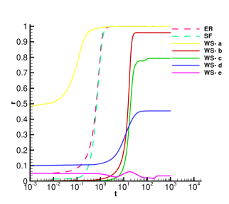
Figure 1: (Color on-line) Order parameter ($r$) versus time (in logarithmic scale) for ER (dashed dark-gray curve), BA (dashed light-gray curve) and WS networks for five different initial conditions (solid curves from top to bottom for WS-a to WS-e, respectively). $N=1000$ and $\langle k\rangle=10$.

Fig.(1) shows the temporal variations of the $r(t)$ on the three types of networks with $N=1000$ and $\langle k\rangle=10$. To obtain these plots, time step is set to $dt=0.01$ and five realizations of initial phase distributions are taken for a fixed network of each type. The rewiring probability for constructing the WS network out of regular one is chosen to be $p=0.04$. As can be seen, the oscillators on ER and BA networks immediately reach to a fully synchronized state ($r=1$) irrespective to the initial conditions. However, in the case of WS network, they more slowly go toward the steady states which are highly dependent on the initial phase distributions in such a way the $r(\infty)$ reaches several values between $0$ and $1$. These results show that in contrast to ER and SF networks, the structure of steady states of the Kuramoto model on SW networks can be more complex. In what follows, we discuss that the sensibility of dynamics to initial conditions is indeed inherited to SW networks from their regular network parents. In a regular network, the ratio of nearest neighbor connections to network size ($k/N$) determines the number of stable solutions. It has been shown that for $k/N<0.34$, different initial conditions lead to different final states reg-basin .

It is easy to show that the stable stationary solutions of Eqs.(2) have to satisfy the following conditions:

$$\sum_{i=1}^{N}\sin\theta_{i}=\sum_{i=1}^{N}\cos\theta_{i}=0,$$ (4)

provided that the phase difference between any two adjacent oscillators be less than $\pi/2$ (i.e, $\Delta\theta_{ij}=\theta_{i}-\theta_{j}<\pi/2$ if $a_{ij}=1$). These solutions can be put in two categories; i)  Full synchronized state with $r=1$ ($\Delta\theta_{ij}=0$ for any $i,j$); ii)  Phase-locked state with regular arrangement of phases around the phase circle with non-zero phase difference $\Delta\theta$, for which $r=0$.
The phase-locked states represent helical wave phase modulations and their number depends on $N$ and $k$. For instants, in the case of $N=1000$ and $k=10$, there are $10$ of such states with nearest neighbor phase differences $\Delta\theta_{nn}^{\alpha}=2\pi/\lambda^{\alpha}$, in which $\lambda^{\alpha}=20,25,40,50,100,125,200,250,500,1000$, are the wavelengths of the helical states indicated by $\alpha=1,2,\cdots 10$, respectively.

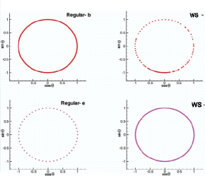
Figure 2: (Color on-line) steady state phase configurations in two helical patterns of regular network and corresponding steady states of WS networks with $N=1000$ and $\langle k\rangle=10$. (b)$\lambda=1000$, and (e)$\lambda=50$. $\lambda$ is the wavelength of helical states in regular network.

The stationary phase configuration of all nodes, corresponding to the initial conditions in Fig.(1), are plotted in Fig.(2), both for the regular and its offspring WS network. This plots corresponds to the helical patterns with phase differences $\lambda=1000,50$, denoted in Fig.(1) by indices, b and e, respectively. This figure shows, rewiring a regular network with phase-locked state, deforms its helical pattern to an inhomogeneous state in the subsequent WS one. Therefore, a WS network possesses various stable stationary states whose number equals the number of helical patterns in its parent regular network.

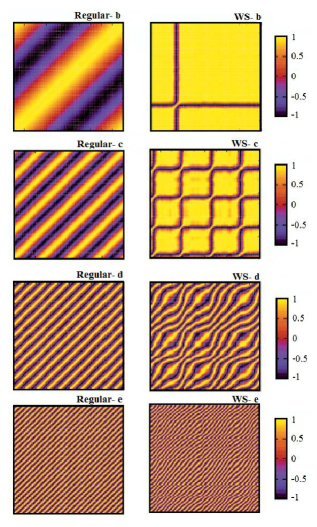
Figure 3: (Color on-line) Density plot of correlation matrix elements ($D_{ij}$) for $4$ helical states of regular network and corresponding stationary states in WS network with $N=1000$ and $\langle k\rangle=10$. (b)$\lambda=1000$, (c)$\lambda=250$, (d)$\lambda=100$ and (e) $\lambda=50$. $\lambda$ is the wavelength of helical states in regular network.

The local structure of the steady state can be better clarified by the correlation matrix $D$ defined as D :

$$D_{ij}=\lim_{\Delta t\rightarrow\infty}\frac{1}{\Delta t}\int_{t_{r}}^{t_{r}+\Delta t}\cos(\theta_{i}(t)-\theta_{j}(t))dt,$$ (5)

in which $t_{r}$ is the time needed for reaching to stationary state. The matrix element $-1\leq D_{ij}\leq 1$ is a measure of coherency between each pair of nodes. In the case of full synchrony between $i$ and $j$ ($\theta_{i}=\theta_{j}$) the correlation matrix element is $D_{ij}=1$ and in the case of anti-phase locking ($\theta_{i}-\theta_{j}=\pi$), the value of matrix element is $D_{ij}=-1$. Fig.(3) represents the density plot of correlation matrix elements for the four steady states of regular and WS networks corresponding to Figs.(1) and (2). This plots clearly show the inhomogeneous structure of the helical patterns before and after rewiring of the regular network. The correlation matrix represents strip structures in its density plot for helical states in regular network and the width of the strips are proportional to the wavelength of the helices. One can also observe from these plots that converting the regular network to WS, the helical patterns are substantially affected, provided $\lambda$ being large. The strip structure of matrix $D$ is almost preserved for small wavelengths, indicating the small wavelength helical patterns, despite of little deformations, are stable against rewiring of network. For large wavelength patterns of regular network, the majority of nodes in the corresponding WS phase configurations are synchronized with each other, however there are some isolated nodes in Anti-phase locking with the rest. These isolated nodes are topological defects and induce spiral phase textures around them, in such a way that the phase of surrounding oscillators varies continuously from $0$ to $\pi$, by getting away from these nodes. The number of these defects increases by decreasing the wavelength of corresponding helical pattern. For example, it can be seen from Fig.(3) that for $\lambda=1000$ there is one while for $\lambda=250$ there are four point defects. Once the structure of the steady states of deterministic Kuramoto model on WS network is known, it would be interesting to investigate the effect of noise on such states.

III The effect of random force

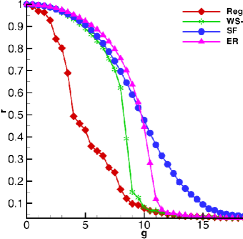
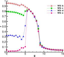
Figure 4: (Color on-line) Stationary order parameter versus reduced noise intensity for the four network types. (top panel): Regular, ER, SF and Full synchronized state of WS. (bottom panel): Four phase locked states of WS corresponding to states represented in Fig.(3). Number of nodes and mean degree for the three networks are $N=1000$ and $\langle k\rangle=10$, respectively.

A network of oscillators could be plagued by some external random forces. The effect of such forces may be modelled by an uncorrelated white noise $(\eta_{i}(t))$ applying to all nodes. Adding this noise to Eq.(2), we have:

$$\dot{\theta}_{i}=K\sum_{j=1}^{N}a_{ij}\sin(\theta_{j}-\theta_{i})+\eta_{i}(t)\;,i=1,\ldots,N\,,$$ (6)

where $\langle\eta_{i}(t)\rangle=0,\langle\eta_{i}(t)\eta_{j}(t^{\prime})\rangle=2D\delta(t-t^{\prime})\delta_{ij}$ with $D$ being the variance or intensity of the noise. In our numerical work, we choose a box distribution in the interval $[-w/2,w/2]$ for $\eta$, so that its variance is equal to $D=w^{2}/24$. It can be shown that by proper re-scaling of the time variable, the effect of parameters $D$ and $K$ can be included in a single parameter $g^{2}=\frac{D}{K}$  khoshbakht , converting the dynamical equations to:

$$\frac{d\theta_{i}}{d\tau}=\sum_{j=1}^{N}a_{ij}\sin(\theta_{j}-\theta_{i})+g\xi_{i}(\tau)$$ (7)

where $\tau=Kt$ is the re-scaled time variable and $\xi_{i}(\tau):=\eta_{i}(t)/g$ is a random variable in the interval $[-1/2,1/2]$.

The numerical integration of Eq.(7) is carried out by employing Euler method for its deterministic part and Ito’s algorithm ito for the stochastic part. Fig.(4) represents the variations of stationary order parameters ($r(\infty)$) versus re-scaled noise intensity $g$, for the four network types regular, SF, ER and WS (top panel for fully synchronized state and bottom panel for phase-locked ones).

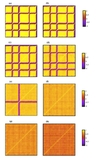
Figure 5: (Color on-line) Density plot of correlation matrix elements ($D_{ij}$) for a steady state with four point defects on SW network and different noise intensities, (a) $g=0$, (b) $g=2$, (c) $g=3$, (d) $g=4$, (e) $g=5$, (f) $g=6$, (g) $g=7$ and (h) $g=8$. Number of nodes and mean degree for the three networks are $N=1000$ and $\langle k\rangle=10$, respectively

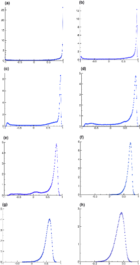
Figure 6: (Color on-line) Probability distribution function of correlation matrix elements ($D_{ij}$) for different noise intensities: (a) $g=0$, (b) $g=2$, (c) $g=3$, (d) $g=4$, (e) $g=5$, (f) $g=6$, (g) $g=7$ and (h) $g=8$. Number of nodes and mean degree for the three networks are $N=1000$ and $\langle k\rangle=10$, respectively.

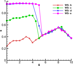
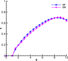
Figure 7: (Color on-line) top: complexity of small world network versus noise intensity for $N=1000$ and $\langle k\rangle=10$. These plots are corresponding to the initial conditions leading to the helical state in parent regular network with wavelength $\lambda=1000,250,100,10$. bottom: complexity of ER and SF networks versus noise intensity for $N=1000$ and $\langle k\rangle=10$.

By inspecting this figure, one can extract two essential results: (i) As can be seen from the top panel, for all the four networks, the order parameter starting from full synchronized state with $r({\infty})=1$, monotonically decreases when the noise is turned on. The critical coupling ($g_{c}$) at which the synchrony disappears among the oscillators is the greatest for SF and the smallest for regular network. Therefore the coherent state in the SF lasts longer against noise than ER, WS and regular with the same average degree and coupling constant. The more fragility of fully synchronized state in regular and WS networks can be explained in terms of the formation of some local clusters in these networks. The phase differences among different clusters of oscillators tend to become large by the effect of random forcing, hence leading to rapid fall of the order parameter. The persistence of synchronized state in SF network has been argued to be related to the existence of few nodes with very large number of connections (hubs) in this type of networks khoshbakht .

(ii) The bottom panel of Fig.(4) shows that for inhomogeneous phase locked states in WS network, variation of $r(\infty)$ versus noise is non-monotonic. It remains almost constant for small noise strengths and reaches to a maximum in an interval of reduced noise intensity. Therefore in these cases, instead of playing destruction role, noise promotes the synchrony among the oscillators.

The noise-induced synchronization is also called stochastic synchronization and its occurrence in WS networks can be explained in terms of defect patterns in the steady states of the Kuramoto model. Fig.(5) represents the evolution of correlation matrix density plots versus reduced noise intensity, $g$, for a specific steady state of WS network with four topological defects. It can be seen in this figure that turning the noise on, the defects resist against the noise up to $g\sim 4$ and for $g>4$ they begin to disappear until $g\sim 6$ where they vanish completely. Disappearance of defects enhances the homogeneity in the system and so the synchrony among the oscillators. This is more apparent in probability distribution of correlation matrix elements ($p(D)$) shown in Fig.(6). As can be seen in this figure, $p(D)$ has two peaks at $D=1,-1$ for $g=0$. Increasing the noise intensity the two peaks move toward each other and at the onset of stochastic synchronization, $g\sim 6$, they emerge in one peak. At this point the variance of $p(D)$ reaches to its minimum and again rises by increasing the noise strength. Fig.(7) represents the complexity of WS, ER and SF networks in terms of reduced noise intensity. The complexity is defined by Shannon entropy of $p(D)$ complexity :

$$S=\left(-\sum_{i=1}^{m}p_{i}\ln p_{i}\right)/\ln m,$$ (8)

in which $m$ is the number of bins in division of $p(D)$ ($m=200$ in this work). This quantity measures both the ability of a network to synchronize as a whole (integration) and in the mean while preserving the independence of its subsystems (segregation). This intermediate regime with high complexity is desirable for functioning of real neural networks.

In top panel of Fig.(7), we compare the complexity of Kuramoto model on WS network for different initial conditions, leading to the patterns shown in Fig.(3). This plot shows that the complexity is larger for the patterns with greater spatial inhomogeneity (corresponding to the helical patterns with smaller wavelength in the regular networks), and these patterns are more robust against noise. By applying the noise, the complexity remains more or less unchanged until the the onset of stochastic synchronization at which shows a sudden fall. Beyond this point, the complexity tends to rise and reaches to a maximum at the noise strength by which the synchronization vanishes. On the contrary, for ER and SF networks, shown in the bottom panel of Fig.(7), the complexity monotonically raises with noise strength and reaches to a maximum at the onset of the vanishing of synchronization.

Finally, we investigate the occurrence of stochastic synchronization in terms of link rewiring probability $p$. We found that value of the noise strength at which the stochastic synchronization occurs, reaches to maximum at $p\sim 0.02$ and then decreases with increasing $p$ and vanishes at $p\sim 0.17$. For $p>0.17$, the behavior of the noisy Kuramoto dynamics on SW network is similar to the random networks. In Fig.(8) we depict the phase diagram for a SW network with $N=1000$ and $\langle k\rangle=10$, in $g-p$ space.

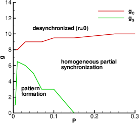
Figure 8: (Color on-line) Phase diagram of noisy Kuramoto model on a SW network with $N=1000$ and $\langle k\rangle=10$, in $g-p$ space. $g_{s}$ (light-gray line) and $g_{c}$ (dark-gray line) denote the noise strengths at the onsets of stochastic synchronization and desynchronization, respectively.

IV conclusion

In summary, we found that a SW network of similar phase oscillators communicating with each other by Kuramoto coupling shows novel behaviors. Unlike ER and SF networks, this system fails to reach a full synchronized state for any arbitrary initial conditions. Moreover, driving it by an uncorrelated white noise, reveals the occurrence of stochastic synchronization, a phenomenon through which a random force induces synchrony among the oscillators. We discussed that the reason for this phenomenon is laid in the stable helical patterns in the regular networks from which the SW ones is built. Rewiring of a regular network of similar phase oscillators with periodic helical pattern, ends to complex inhomogeneous states in the resulting SW network. The existence of such stable inhomogeneous patterns in SW network, appearing some times as topological point defects and also as aperiodic helical patterns, prevents the network from reaching to full synchrony. These patterns persist against the noise for small noise intensities. However the external random forces with moderate strengths are able to destroy these patterns in favor of more homogeneous states, hence enhance the synchronization among oscillators. We computed the complexity on the SW network in the case of the inhomogeneous pattern formation, and showed that the complexity of such states are larger than the ER and SF networks, for the noise strength less than the onset of stochastic synchronization. Therefore, as a model for neural networks, this finding shows that the functioning of such systems can be more efficient in the presence of a moderate noise. Generalization of the above results to the more realistic case in which the coupling constants (coefficients of periodic couplings) are normalized to the degree of the nodes, is currently under investigation. We hope our results may shed light on the fact that why SW networks are so ubiquitous in natural systems.

- (1) F. Sagués, J. M. Sancho, and J. García-Ojalvo, Rev. Mod. Phys 79, 829 (2007).
- (2) L. Gammaitoni, P. Hnggi, P. Jung, and F. Marchesoni, Rev. Mod. Phys 70, 223 (1998).
- (3) B. Lindner, J. García-Ojalvo, A. Neiman, and L. Schimansky-Geier, Phys. Rep. 392, 321 (2004).
- (4) P. Reimann, Phys. Rep. 361, 57 (2002).
- (5) W. Horsthemke, and R. Lefever, Noise-Induced Transitions, (Springer, Berlin, 1984).
- (6) S. Kádár, J. Wang, and K. Showalter, Nature (London) 391, 770 (1998); S. Alonso, I. Sendia-Nadal, V. Prez-Muuzuri, J. M. Sancho, and F. Sagus , Phys. Rev. Lett. 87 078302 (2001); S. Tanabe, and K. Pakdaman, Biol. Cybern. 85 269 (2001); C. J. Tessone, A. Scir , R. Toral , and P. Colet, Phys. Rev. E 75 016203 (2007).
- (7) W. H. Calvin, and C. F. Stevens, Science 155 842 (1967).
- (8) G. B. Ermentrout, R. F. Galán, and N. N. Urban, Trends in Neuroscience 31 428 (2008).
- (9) A. N. Burkitt, and G. M. Clark, Neural Comput. 11, 871 (1999); E. Salinas, and T. J. Sejnowski, Nat. Rev. Neurosci. 2, 539 (2001); A. D. Reyes, Nat. Neurosci. 6, 593 (2003); P. H. Tiesinga, and T. J. Sejnowski, Neural Comput. 16, 251 (2004).
- (10) M. Stopfer et al, Nature 390, 70 (1997); A. K. Engel et al, Conscious Cogn. 8, 128 (1999); M. N. Shadlen, and J. A. Movshon, Neuron 24, 67 (1999); J. A. Movshon, Neuron 27, 412 (2000).
- (11) M. Springer, and J. Paulsson, Nature 439, 27 (2006); T. Zhou, L. Chen, and K. Aihara, Phys. Rev. Lett. 95, 178103 (2005).
- (12) A. Arenas, A. Diaz-Guilera, J. Kurths, Y. Moreno and C. Zhou, Physics Reports 469, 93-153 (2008).
- (13) Y. Kuramoto, Lecture Notes Physics (Springer, New York, 1975), Vol. 39, pp. 420-422; Y. Kuramoto, Chemical Oscillations, Waves, and Turbulence (Springer, Berlin, 1984).
- (14) J. A. Acebrón, L. L. Bonilla, and Conrad J. Pérez Vicente, Félix Ritort, and R. spigler, Rev. Mod. Phys. 77, 137 (2005); B. C. Bag, K. G. Petrosyan, and Hu Chin-Kun, Phys. Rev. E 76, 056210 (2007);
- (15) H. Khoshbakht, F. Shahbazi, and, K. Aghababaei Samani, J. Stat. Mech, P10020 (2008).
- (16) J. D. Watts, and S. H. Strogatz, Nature 393, 440 (1998).
- (17) S. H. Strogatz, Nature 410, 268 (2001).
- (18) Z. Gao, B. Hu, and G. Hu, Phys. Rev. E 65, 016209 (2001); H. Hong, B. J. Kim, and M. Y. Choi, ibid. 66, 011107 (2002) ; M. Perc, and M. Gosak, New J. Phys. 10, 053008 (2008) .
- (19) O. Kwon, and H.-T. Moon, Phys. Lett A 298, 319 (2002); O. Kwon, H.-H. Jo , and H.-T. Moon , Phys. Rev. E 72, 066121(2005).
- (20) D. S. Bassett, and E. Bullmore, The Neuroscientist 12, 512 (2006); E. Bullmore, and O. Sporns, Nature Reviews Neuroscience 10, 186 (2009).
- (21) H. Hong, M. Y. Choi, and B. J. Kim, Phys. Rev. E 65, 026139 (2002).
- (22) A. L. Barabási, and R. Albert, Science 286, 509 (1999); A. L. Barabasi, R. Albert, and H. Joeng, Physica A 272, 173 (1999).
- (23) P. Erdös, and A. Rényi, Publ. Math. Debrecen 6, 290 (1959); Publ. Math. Inst. Hung. Acad. Sci 5, 17 (1960).
- (24) A. D. Wiley, S. H. Strogatz, and M. Girvan, Chaos 16, 015103 (2006) .
- (25) J. Gómez-Gardees, Y. Moreno, and A. Arenas, Phys. Rev. Lett. 98, 034101 (2007).
- (26) C. W. Gardiner, Handbook of Stochastic Methods for Physics, Chemistry and the Natural Sciences, (Springer-Verlag, 1980).
- (27) M. Zhao, C. Zhou, Y. Chen, B. Hu, and B-H. Wang, Phys. Rev E 82, 046225 (2010).