Conformal Wasserstein Distance:
II. Computational Aspects and Extensions

Abstract.

This paper is a companion paper to [19]. We provide numerical procedures and algorithms for computing the alignment of and distance between two disk type surfaces. We provide a convergence analysis of the discrete approximation to the arising mass-transportation problems. We furthermore generalize the framework to support sphere-type surfaces, and prove a result connecting this distance to local geodesic distortion. Lastly, we provide numerical experiments on several surfaces’ datasets and compare to state of the art method.

1. introduction and background

Alignment of surfaces plays a role in a wide range of scientific disciplines. It is a standard problem in comparing different scans of manufactured objects; various algorithms have been proposed for this purpose in the computer graphics literature. It is often also a crucial step in a variety of problems in medicine and biology; in these cases the surfaces tend to be more complex, and the alignment problem may be harder. For instance, neuroscientists studying brain function through functional Magnetic Resonance Imaging (fMRI) typically observe several people performing identical tasks, obtaining readings for the corresponding activity in the brain cortex of each subject. In a first approximation, the cortex can be viewed as a highly convoluted 2-dimensional surface. Because different cortices are folded in very different ways, a synthesis of the observations from different subjects must be based on appropriate mappings between pairs of brain cortex surfaces, which reduces to a family of surface alignment problems [9, 28]. In another example, paleontologists studying molar teeth of mammals rely on detailed comparisons of the geometrical features of the tooth surfaces to distinguish species or to determine similarities or differences in diet [2].

Mathematically, the problem of surface alignment can be described as follows: given two 2-surfaces $\mathcal{M}$ and $\mathcal{N}$, find a mapping $f:\mathcal{M}\rightarrow\mathcal{N}$ that preserves, as best possible, “important properties” of the surfaces. The nature of the “important properties” depends on the problem at hand. In this paper, we concentrate on preserving the geometry, i.e., we would like the map $f$ to preserve intrinsic distances, to the extent possible. In terms of the examples listed above, this is the criterion traditionally selected in the computer graphics literature; it also corresponds to the point of view of paleontologists studying tooth surfaces. To align cortical surfaces, one typically uses the Talairach method [18] (which relies on geometrically defined landmarks and is thus geometric in nature as well), although alignment based on functional correspondences has been proposed more recently [28].

In [19] a novel procedure between disk type surfaces was proposed, based on uniformization theory and optimal mass transportation. In a nutshell, the method maps two surfaces $\mathcal{M},\mathcal{N}$ to densities $\mu,\nu$ (interpreted as mass densities) defined on the hyperbolic disk $\mathcal{D}=\left\{z\mid\left|z\right|<1\right\}$ , their canonical uniformization space. (Apart from simplifying the description of the surface, this also removes any effect of global translations and rotations on the description of each individual surface.) The alignment problem can then be studied in the framework of Kantorovich mass-transportation [16] between these metric densities. Mass-transportation seeks to minimize the “average distance” over which mass needs to be “moved” (in the most efficient such moving procedure) to transform one mass density $\mu$ into another, $\nu$:

(1.1) $$T_{c}(\mu,\nu)=\mathop{\inf}_{\pi\in\Pi(\mu,\nu)}\int_{\mathcal{D}\times\mathcal{D}}c(z,w)d\pi(z,w),$$

where $c(z,w)\geq 0$ is a cost function, and $\Pi(\mu,\nu)$ is the collection of probability measures on $\mathcal{D}\times\mathcal{D}$ with marginals $\mu$ and $\nu$ (resp.), that is, for $A\subset\mathcal{D}$, $B\subset\mathcal{D}$, $\pi(A\times\mathcal{D})=\mu(A)$ and $\pi(\mathcal{D}\times B)=\nu(B)$.

In our case the uniformizing metric density (or conformal factor) corresponding to an initial surface is not unique, but is defined only up to a Möbius transformation. Because a naïve application of mass-transportation on the hyperbolic disk would not possess the requisite invariance under Möbius transformations, we generalize the mass-transportation framework, and replace the cost function $d(z,w)$ traditionally used in defining the “average displacement distance” by a cost that depends on $\mu$ and $\nu$, $d^{R}_{\mu,\nu}(z,w)$, measuring the dissimilarity between the two metric densities on $R$-neighborhoods of $z$ and $w$ (where $R$ is a parameter that controls the size of the neighborhoods):

(1.2) $$T^{R}_{d}(\mu,\nu)=\mathop{\inf}_{\pi\in\Pi(\mu,\nu)}\int_{\mathcal{D}\times\mathcal{D}}d^{R}_{\mu,\nu}(z,w)d\pi(z,w).$$

Introducing neighborhoods also makes the definition less sensitive to noise in practical applications. The optimal way of transporting mass in this generalized framework defines a corresponding optimal way of aligning the surfaces. This approach also allows us to define a new distance, $\mbox{\bf{d}}^{R}(\mathcal{M},\mathcal{N})$, between surfaces; the average distance over which mass needs transporting (to transform one metric density into the other) quantifies the extent to which the two surfaces differ.

This paper contains three contributions that complement and extend [19]. The first of these is to provide an algorithm for approximating $\mbox{\bf{d}}^{R}(\mathcal{M},\mathcal{N})$ and to prove a convergence result for this algorithm. In order to state this goal more precisely, we introduce some technicalities and notations now.

1.1. Uniformization

Uniformization theory for Riemann surfaces [31, 14] allows conformally flattening disk type surfaces onto the unit disk $\phi:\mathcal{M}\rightarrow\mathcal{D}$ in $\mathbb{C}$, where $\phi$ is the conformal flattening map, $\mathcal{D}=\{z\ |\ |z|<1\}$ is the unit disk, and the disk coordinate system is denoted by $z=x^{1}+\textbf{\footnotesize{i}}x^{2}$. The surface’s Riemannian metric $g$ is then pushed-forward to a diagonal metric tensor

$$\widetilde{g}=\phi_{*}g=\mu^{E}(z)\,\delta_{ij}\,dx^{i}\otimes dx^{j},$$

where $\mu^{E}(z)>0$, Einstein summation convention is used, and the subscript $*$ denotes the “push-forward” action; the superscript $E$ stands for Euclidean. The function $\mu^{E}$ can also be viewed as the density function of the measure $\mbox{\rm{vol}}_{\mathcal{M}}$ induced by the Riemann volume element: for (measurable) $A\subset\mathcal{M}$,

(1.3) $$\mbox{\rm{vol}}_{\mathcal{M}}(A)=\int_{\phi(A)}\mu^{E}(z)\,d\mbox{\rm{\footnotesize{vol}}}_{E}(z),$$

where $d\mbox{\rm{\footnotesize{vol}}}_{E}(z)=dx^{1}\wedge dx^{2}$ is the Euclidean area element . For a second surface $\mathcal{N}$ with Riemannian metric $h$ we will denote its pushed-forward metric on the uniformization disk $\mathcal{D}$ by $\widetilde{h}=\phi_{*}h=\nu^{E}(w)\,\delta_{ij}\,dy^{i}\otimes dy^{j},$ where the coordinates in the unit disk are $w=y^{1}+\textbf{\footnotesize{i}}y^{2}$.

We use the hyperbolic metric on the unit disk $(1-|z|^{2})^{-2}\delta_{ij}dx^{i}\otimes dx^{j}$ as a reference metric; the surface density w.r.t. the hyperbolic metric (conformal scaling) is

(1.4) $$\mu^{H}(z):=(1-|z|^{2})^{2}\,\mu^{E}(z)\,,$$

where the superscript $H$ stands for hyperbolic.

We shall often drop this superscript: unless otherwise stated $\mu=\mu^{H}$, and $\nu=\nu^{H}$ in what follows. The density function $\mu=\mu^{H}$ satisfies

$$\mbox{\rm{vol}}_{\mathcal{M}}(A)=\int_{\phi(A)}\mu(z)\,d\mbox{\rm{\footnotesize{vol}}}_{H}(z)\,,$$

where $d\mbox{\rm{\footnotesize{vol}}}_{H}(z)=(1-|z|^{2})^{-2}\,d\mbox{\rm{\footnotesize{vol}}}_{E}(z)$. We will use the notations $\mu,\nu$ also to represent the measures $\mbox{\rm{vol}}_{\mathcal{M}},\mbox{\rm{vol}}_{\mathcal{N}}$ (resp.), where the exact meaning will be clear from the context.

The conformal mappings of $\mathcal{D}$ to itself are the disk-preserving Möbius transformations, they constitute the group $M_{\mathcal{D}}$ of isometries of the hyperbolic disk. An arbitrary element $m\in M_{\mathcal{D}}$ is characterized by three real parameters:

(1.5) $$m(z)=e^{\textbf{\footnotesize{i}}\theta}\frac{z-a}{1-\bar{a}z},\ a\in\mathcal{D},\ \theta\in[0,2\pi).$$

The pull-back $m^{*}\mu(z)$ and the push-forward $m_{*}\mu(w)$ of the density $\mu$ by the Möbius transformation $m$ are given by the formulas

(1.6) $$m^{*}\mu(z)=\mu(m(z)),$$

and

(1.7) $$m_{*}\mu(w)=\mu(m^{-1}(w)),$$

respectively.

It follows that checking whether or not two surfaces $\mathcal{M}$ and $\mathcal{N}$ are isometric, or searching for isometries between $\mathcal{M}$ and $\mathcal{N}$, is greatly simplified by considering the conformal mappings from $\mathcal{M}$, $\mathcal{N}$ to $\mathcal{D}$: once the (hyperbolic) density functions $\mu$ and $\nu$ are known, it suffices to identify $m\in M_{\mathcal{D}}$ such that $\nu(m(z))$ equals $\mu(z)$ (or “nearly” equals, in a sense to be made precise).

1.2. Optimal volume transportation for surfaces

To adapt the optimal transportation framework to the alignment of surfaces, we use an isometry invariant cost function $d^{R}_{\mu,\nu}(z,w)$ that is plugged into the transportation framework (1.1). This special cost function $d^{R}_{\mu,\nu}(z,w)$ indicates the extent to which a neighborhood of the point $z$ in $(\mathcal{D},\mu)$, the (conformal representation of the) first surface, is isometric with a neighborhood of the point $w$ in $(\mathcal{D},\nu)$, the (conformal representation of the) second surface. Two definitions are in order: 1) the neighborhoods we will use, and 2) how we characterize the (dis)similarity of two neighborhoods, equipped with different metrics.

For the neighborhoods, we take the hyperbolic geodesic disks $\Omega_{z_{0},R}$ of radius $R$, where we let $z_{0}$ range over $\mathcal{D}$, but keep the radius $R>0$ fixed. The following gives an easy procedure to construct these disks. If $z_{0}=0$, then the hyperbolic geodesic disks centered at $z_{0}=0$ are also “standard” (i.e. Euclidean) disks centered at 0: $\Omega_{0,R}=\{z\,;\,|z|\leq r_{R}\}$, where $r_{R}=\mbox{tanh}(R)$. The hyperbolic disks around other centers are images of these central disks under Möbius transformations (= hyperbolic isometries): setting $m(z)=(z-z_{0})(1-z\bar{z_{0}})^{-1}$, we have

(1.8) $$\Omega_{z_{0},R}=m^{-1}(\Omega_{0,R})\,.$$

Next, the (dis)similarity of the pairs $\left(\Omega_{z_{0},R}\,,\,\mu\,\right)$ and $\left(\Omega_{w_{0},R}\,,\,\nu\,\right)$ is defined via pull-back of $\nu$ and using the standard induced norm (see [19] for more details). The final cost function is achieved by taking the infimum over all Möbius transformations $m$ such that $m(z)=w$:

(1.9) $$d^{R}_{\mu,\nu}(z_{0},w_{0}):=\mathop{\inf}_{m\in M_{\mathcal{D}}\,,\,m(z_{0})=w_{0}}\int_{\Omega_{z_{0},R}}\,|\,\mu(z)-(m^{*}\nu)(z)\,|\,d\mbox{\rm{\footnotesize{vol}}}_{H}(z),$$

where $d\mbox{\rm{\footnotesize{vol}}}_{H}(z)=(1-|z|^{2})^{-2}\,dx^{1}\wedge dx^{2}$ is the volume form for the hyperbolic disk.

As proved in [19] $d^{R}_{\mu,\nu}(\cdot,\cdot)$ is a metric on $\mathcal{D}$ and as a consequence

(1.10) $$\mbox{\bf{d}}^{R}(\mathcal{M},\mathcal{N})=T^{R}_{d}(\mu,\nu)$$

(with $T^{R}_{d}(\mu,\nu)$ as defined in 1.2) defines a semi-metric in the space of disk-type surfaces. To ensure that this is a metric rather than only a semi-metric, we add an extra assumption, namely that no (orientation-preserving) self-isometries exist within each of the compared surfaces. For discussion and more detail we refer the reader to [19].

1.3. Overview

We can now formulate a precise overview of the algorithm for approximating $\mbox{\bf{d}}^{R}(\mathcal{M},\mathcal{N})$, and discuss its convergence properties.

In a nutshell, the key steps of the algorithm are: 1) approximate uniformization for piecewise linear surface representations, 2) discretize the continuous measures $\mu,\nu$ based on discrete sample sets $Z=\left\{z_{i}\right\}_{i=1}^{n},W=\left\{w_{j}\right\}_{j=1}^{p}$, obtaining discrete measures by $\mu_{Z},\nu_{W}$ (resp.), 3) approximate the measure-dependent cost function $\breve{d}^{R}_{\mu,\nu}(z,w)\approx d^{R}_{\mu,\nu}(z,w)$, and 4) calculate the discrete optimal transportation cost $T_{\breve{d}}^{R}(\mu_{Z},\nu_{W})$ between the discrete measures $\mu_{Z},\nu_{W}$ based on the approximated cost function $\breve{d}^{R}_{\mu,\nu}(z,w)$.

In the heart of our analysis we prove the convergence $T_{\breve{d}}^{R}(\mu_{Z},\nu_{W})\rightarrow\mbox{\bf{d}}^{R}(\mathcal{M},\mathcal{N})$ as the “mesh size” of the samplings used in steps 2, 3 and 4, tend to zero. More precisely, we define the fill distance $\varphi_{g}(Z)$ for the metric tensor $g$ and the sample set $Z$ as

(1.11) $$\varphi_{g}(Z)\,:=\,\sup\left\{r>0\ \big{|}\ z\in\mathcal{M}:B_{g}(z,r)\cap Z=\emptyset\right\}~{},$$

where $B_{g}(z,r)$ is the geodesic open ball of radius $r$ centered at $z$. That is, $\varphi_{g}(Z)$ is the radius of the largest geodesic ball that can be fitted on the surface $\mathcal{M}$ without including any point of $Z$. The smaller $\varphi_{g}(Z)$, the finer the sampling set. We prove the following theorem:

Theorem 1.1.

Let $\mu,\nu$ be Lipschitz continuous probability densities (w.r.t the hyperbolic measure) defined over $\mathcal{D}$. Let $\mathcal{M},\mathcal{N}$ be the disk-type surfaces defined by the metric tensors $g=\mu(z)\,(1-|z|^{2})^{-2}\delta_{ij}dx^{i}\otimes dx^{j},h=\nu(w)\,(1-|w|^{2})^{-2}\delta_{ij}dy^{i}\otimes dy^{j}$ (resp.), let $Z,W$ be discrete sample sets on $\mathcal{M},\mathcal{N}$ (resp.), $\left\{p_{k}\right\}$ samples in $\mathcal{D}$ used for numerical integration, and let $L$ be the number of uniformly spaced points on the circle used to define $T_{\breve{d}}^{R}$ (see below). Then

$$\Big{|}\mbox{\bf{d}}^{R}(\mathcal{M},\mathcal{N})-T^{R}_{\breve{d}}(\mu_{Z},\nu_{W})\Big{|} = \Big{|}T^{R}_{\breve{d}}(\mu,\nu)-T^{R}_{\breve{d}}(\mu_{Z},\nu_{W})\Big{|}$$

$$\leq \omega_{d^{R}_{\mu,\nu}}\left(2\max\left(\varphi_{g}(Z),\varphi_{h}(W)\right)\right)+C_{1}\varphi_{E}\left(\left\{p_{k}\right\}\right)+C_{2}\,L^{-1}\,+\,\epsilon_{\mbox{\tiny{\rm unif}}},$$

where

$$\omega_{d^{R}_{\mu,\nu}}(t)=\sup_{d_{\mathcal{M}}(z,z^{\prime})+d_{\mathcal{N}}(w,w^{\prime})<t}\left|d^{R}_{\mu,\nu}(z,w)-d^{R}_{\mu,\nu}(z^{\prime},w^{\prime})\right|.$$

denotes the modulus of continuity of the cost function $d^{R}_{\mu,\nu}$, and $C_{1},C_{2}$ are constants that depend only upon $\mu,\nu,R$.

Here $\varphi_{E}\left(\left\{p_{k}\right\}\right)$ and $L^{-1}$ are two algorithm parameters that can be made arbitrary small. The error term $\epsilon_{\mbox{\tiny{\rm unif}}}$ concerns only the approximations made in the discrete uniformizations for each of the two surfaces, separately; we’ll come back to it below – suffice it to say here that it is much smaller than the other error terms, in practice. Finally, it was proved in [19] that the cost function $d^{R}_{\mu,\nu}(z,w)$ is uniformly continuous on $\overline{\mathcal{D}}\times\overline{\mathcal{D}}$ and therefore $\omega_{d^{R}_{\mu,\nu}}\left(2\max\left(\varphi_{g}(Z),\varphi_{h}(W)\right)\right)\rightarrow 0$ as the fill-distances of the sets $Z,W$ go to zero.

Two comments are in order: first, we believe that the cost function $d^{R}_{\mu,\nu}(z,w)$ is Lipschitz rather than just uniformly continuous. If this is the case, then our analysis guarantees linear convergence of the algorithm (leaving aside the $\epsilon_{\mbox{\tiny{\rm unif}}}$ term). We leave checking the precise regularity of the cost function to future work. Second, we should discuss in more detail $\epsilon_{\mbox{\tiny{\rm unif}}}$, containing the errors produced from the discrete uniformization. One typically starts from a piecewise flat approximation of the surfaces $\mathcal{M},\mathcal{N}$, given by triangle meshes with a very fine mesh size, providing much finer sampling than the $Z$ or $W$ used in steps 2 through 4. (For instance, in our numerical computations, the parameter $L$ and the sample sets $Z,W$ were picked so that $L^{-1}$, $\varphi_{g}(Z),\,\varphi_{h}(W)$ had magnitude .02,.06,.06 (resp.); the mesh size in the original triangulation of $\mathcal{M},\,\mathcal{N}$ is of order .01.) How to construct discrete approximations of the uniformization of the surfaces, starting from these approximations to $\mathcal{M},\,\mathcal{N}$, is a research area in its own right, and several different methods have been proposed [12, 26, 30]; in our work we adopt the approach of [26, 20]. The error $\epsilon_{\mbox{\tiny{\rm unif}}}$ contributed by this component of our algorithm is governed by the difference between the “true” $\mu,\nu$ and the $\mu^{approx},\nu^{approx}$ stemming from the discrete triangulation approximation, followed by the discrete uniformization, and is bounded by (using the triangle inequality proved in Theorem 3.11 in [19])

$$\epsilon_{\mbox{\tiny{unif}}}\leq T_{d}^{R}(\mu,\mu^{approx})+T^{R}_{d}(\nu,\nu^{approx}).$$

We expect this difference to be proportional to the triangulation mesh size, and to be negligible compared to the errors we analyze explicitly in this paper. Since the convergence analysis of discrete uniformization has not settled yet into its final form, and given the much smaller size of this component of the error (both expected and borne out by numerical experiments), we have opted here to view the discrete uniformization as a “black box”, the analysis of which is outside the scope of this paper, and to neglect this part of the error. We concern ourselves here with the error made by our algorithm in the approximation to $T_{d}^{R}(\mu^{approx},\nu^{approx})$, namely with

$$\Big{|}T_{d}^{R}(\mu^{approx},\nu^{approx})-T_{d}^{R}(\mu_{Z},\nu_{W})\Big{|}\,.$$

We now turn to the other contributions made by this paper. In an earlier version of the paper, Theorem 2.4 was the main result. Interesting questions and challenges by the reviewers led us to investigate extensions and further mathematical properties of our construction; the results are formulated as two further contributions.

The first of these is a generalization of the framework above to other types of surfaces. We show how a similar distance $\mbox{\bf{d}}^{A}(\mathcal{M},\mathcal{N})$ can be defined for genus-zero, or sphere-type surfaces. This involves some new ideas, since the absence of a distance function on the sphere $S^{2}$ that would be invariant under all conformal maps from $S^{2}$ to itself, implies that the definitions of the neighborhoods $\Omega_{z_{0},R}$ cannot simply be copied from the case for disk-type surfaces.

The final contribution of this paper concerns possible connections between the distance $\mbox{\bf{d}}^{R}(\mathcal{M},\mathcal{N})$ and the notion of geodesic distortion. Although there is certainly much more to be said upon this topic than we do here, we do present a first result, showing that if the distance $\mbox{\bf{d}}^{R}(\mathcal{M},\mathcal{N})$ between two disk-like surfaces is small, then the two surfaces are locally near-isometric. More precisely, we prove the following:

Theorem 1.2.

Let $\mathcal{M}$ and $\mathcal{N}$ be differentiable disk-like surfaces. If $\mbox{\bf{d}}^{R}(\mathcal{M},\mathcal{N})$ is sufficiently small, then we can cover $\mathcal{M}$ (minus an arbitrarily small boundary layer) with patches $\Omega_{z_{0},R}$ and define mappings $f^{z_{0}}:\mathcal{M}\rightarrow\mathcal{N}$ (Möbius transformations) such that for all $z_{1},z_{2}\in\mathcal{M}$ (not very close to the boundary) with geodesic distance $d_{g}(z_{1},z_{2})\leq r(R)$, $r(R)>0$, there exists a patch $\Omega_{z_{0},R}$ such that $z_{1},z_{2}\in\Omega_{z_{0},R}$, and

(1.12) $$\left(1-C_{2}\mbox{\bf{d}}^{R}(\mathcal{M},\mathcal{N})^{1/3}\right)d_{g}(z_{1},z_{2})\leq d_{h}(f^{z_{0}}(z_{1}),f^{z_{0}}(z_{2}))\leq\left(1+C_{1}\mbox{\bf{d}}^{R}(\mathcal{M},\mathcal{N})^{1/3}\right)d_{g}(z_{1},z_{2}),$$

where $d_{g}(z_{1},z_{2}),d_{h}(w_{1},w_{2})$ are the geodesic distances of $z_{1},z_{2}\in\mathcal{M}$ and $w_{1},w_{2}\in\mathcal{N}$, respectively, and $C_{1},C_{2}>0$ are constants independent of the choice of $z_{1},z_{2}$.

1.4. Related work

The approach taken in this paper is related to the computer graphics constructions in [20], which rely on the representation of isometries between topologically equivalent simply-connected surfaces by Möbius transformations between their uniformization spaces, and which exploit that 1) the Möbius group has small dimensionality (e.g. 3 for disk-type surfaces and 6 for sphere-type) and 2) changing the metric in one piece of a surface has little influence on the uniformization of distant parts. These two observations lead, in [20], to fast and effective algorithms to identify near-isometries between differently deformed versions of a surface. In our present context, these same observations lead to a simple algorithm for surface alignment, reducing it to a linear programming problem.

Other distances between surfaces have been used recently for several applications [21]. A prominent mathematical approach to define distances between surfaces considers the surfaces as special cases of metric spaces, and uses then the Gromov-Hausdorff (GH) distance between metric spaces [11]. The GH distance between metric spaces $X$ and $Y$ is defined through examining all the isometric embedding of $X$ and $Y$ into (other) metric spaces; although this distance possesses many attractive mathematical properties, it is inherently hard computationally [22, 1]. For instance, computing the GH distance is equivalent to a non-convex quadratic programming problem; solving this directly for correspondences is equivalent to integer quadratic assignment, and is thus NP-hard [6]. In addition, the non-convexity implies that the solution found in practice may be a local instead of a global minimum, and is therefore not guaranteed to give the correct answer for the GH distance. The distance between surfaces as we define in [19] does not have these shortcomings because the computation of the distance between surfaces using this approach can be recast as a linear program, and can therefore be implemented using efficient polynomial algorithms that are moreover guaranteed to converge to the correct solution.

In [21], the GH distance of [22] is generalized by introducing a quadratic mass transportation scheme to be applied to metric spaces equipped with a measure (mm spaces); the computation of this Gromov-Wasserstein distance for mm spaces is somewhat easier and more stable to implement than the original GH distance [21]. A crucial aspect in which our work differs from [21] is that, in contrast to the (continuous) quadratic programming method proposed in [21] to compute the Gromov-Wasserstein distance between mm spaces, our conformal approach leads to a convex (even linear) problem, solvable via a linear programming method.

It is worth mentioning that optimal mass transportation has been used in the engineering literature as well, to define interesting metrics between images; in this context the metric is often called the Wasserstein distance. The seminal work for this image analysis approach is the paper by Rubner et al. [27], in which images are viewed as discrete measures, and the distance is called appropriately the “Earth Mover’s Distance”.

Another related method is presented in the papers of Zeng et al. [33, 34], which also use the uniformization space to match surfaces. Our work differs from that of Zeng et al. in that they use prescribed feature points (defined either by the user or by extra texture information) to calculate an interpolating harmonic map between the uniformization spaces, and then define the final correspondence as a composition of the uniformization maps and this harmonic interpolant. This procedure is highly dependent on the prescribed feature points, provided as extra data or obtained from non-geometric information. In contrast, our work does not use any prescribed feature points or external data, and makes use of only the geometry of the surface; in particular we utilize the conformal structure itself to define deviation from (local) isometry.

1.5. Organization

Section 2 presents the main steps for the discretization of the continuous case and provides algorithmic aspects for the alignment procedure. Section 3 generalizes the method to sphere-type surfaces. Section 4 provides a theoretical result connecting our distance directly to local geodesic distortion. Section 5 presents experimental validation of the algorithms and concludes; in particular, we report results of the method applied to various benchmark data sets and provide a comparison to a state-of-the-art method. This paper also contains four appendices: A) contains few approximation results used by our algorithm, B) contains background on the discrete conformal mapping we use, C) contains proofs of some properties of the linear program solution, and D) contains the approximation analysis of the discrete optimal transport cost to its continuous counterpart.

2. Algorithm for comparing disk-type surfaces and analysis

Transforming the theoretical framework discussed above into an algorithm requires several steps of approximation. Our general plan is to recast the transportation eq. (1.2) as a linear programming problem between discrete measures. The steps of our algorithm are as follows:
Preprocess: approximating the surfaces’ uniformization,
Step 1: discretizing the resulting continuous measures,
Step 2: approximating the cost function $d^{R}_{\mu,\nu}(\cdot,\cdot)$,
Step 3: solving a linear programming problem to achieve the final approximation of the distance, and the optimal transportation plan (correspondences).
Step 4 (optional): extract a consistent set of correspondences.

In the following we describe in detail each of these steps; we also provide a convergence analysis for steps 1-3, but not for the preprocess step. (As explained in the introduction the convergence of the approximated uniformization is not the focus of this paper, and we consider it as a ”black box”.) For the sake of completeness, and as a guide to readers who would like to implement the algorithm, we nevertheless include a description of this part in Appendix B.

2.1. Step 1: Discretizing continuous measures

In this subsection we indicate how to construct the discrete measures $\mu_{Z},\nu_{W}$ used in further steps.

Given the measure $\mu=\mbox{\rm{vol}}_{\mathcal{M}}$ on $\mathcal{D}$, we discretize it by first distributing $n$ points $Z=\left\{z_{i}\right\}_{i=1}^{n}$ “uniformly w.r.t. $\mu$”. Details on the particular algorithm we used for sampling are provided in Appendix B (we use the same technique for the sets $Z,W$ described there). For $i=1,\ldots,n$, we define the sets $\left\{\Xi_{i}\right\}_{i=1}^{n}$ to be the Voronoi cells corresponding to $z_{i}\in Z$ defined by the metric of $\mathcal{M}$; this gives a partition of $\mathcal{D}$ into disjoint sets, $\mathcal{D}=\cup_{i=1}^{n}\Xi_{i}$. For a more detailed definition of Voronoi cells as-well as properties of the discrete measures see Appendix D. Next, define the discrete measure $\mu_{Z}$ as a superposition of delta measures localized in the points of $Z$, with weights given by the areas of $\Xi_{i}$, i.e.

(2.1) $$\mu_{Z}\,=\,\sum_{i=1}^{n}\,\mu_{i}\delta_{z_{i}},$$

with $\mu_{i}:=\mbox{\rm{vol}}_{\mathcal{M}}(\Xi_{i})=\int_{\Xi_{i}}\mu(z)d\mbox{\rm{\footnotesize{vol}}}_{H}$. Similarly we denote by $W=\{w_{j}\}_{j=1}^{p}$, $\left\{\Upsilon_{j}\right\}_{j=1}^{p}$, $\nu_{W}$, and $\nu_{j}:=\mbox{\rm{vol}}_{\mathcal{N}}(\Upsilon_{j})$ the corresponding quantities for the measure $\nu=\mbox{\rm{vol}}_{\mathcal{N}}$.

We shall always assume that the surfaces $\mathcal{M}$ and $\mathcal{N}$ have the same area, which, for convenience, we can take to be 1. It then follows that the discrete measures $\mu_{Z}$ and $\nu_{W}$ have equal total mass (regardless of whether $n=p$ or not). The approximation algorithm will compute optimal transport for the discrete measures $\mu_{Z}$ and $\nu_{W}$; the corresponding discrete approximation to the distance between $\mathcal{M}$ and $\mathcal{N}$ is then given by $T^{R}_{d}(\mu_{Z},\nu_{W})$.

The convergence analysis we present will be in terms of the fill distance $\varphi_{g}(Z),\varphi_{h}(W)$ defined in the introduction. Note that our analysis will work with any point sample sets as long as their fill distances converge to zero.

2.2. Step 2: approximating the cost function $d^{R}_{\mu,\nu}$.

In order to approximate $T_{d}^{R}(\mu_{Z},\nu_{W})$ we need to approximate the cost function $d^{R}_{\mu,\nu}(z,w)$ between pairs of points $(z_{i},w_{j})\in Z\times W$.

Applying (1.9) to the points $z_{i}$, $w_{j}$ we have:

(2.2) $$d^{R}_{\mu,\nu}(z_{i},w_{j})=\min_{m(z_{i})=w_{j}}\int_{\Omega_{z_{i},R}}\Big{|}\,\mu(z)-\nu(m(z))\,\Big{|}\,d\mbox{\rm{\footnotesize{vol}}}_{H}.$$

To obtain $d^{R}_{\mu,\nu}(z_{i},w_{j})$ we will thus need to approximate integrals over hyperbolic disks of radius $R$, which is done via a separate approximation procedure, set up once and for all in a preprocessing step at the start of the algorithm.

By using a Möbius transformation $\widetilde{m}$ such that $\widetilde{m}(0)=z_{0}$, and the identity

$$\int_{\Omega_{z_{0},R}}\Big{|}\,\mu(z)-\nu(m(z))\,\Big{|}\,d\mbox{\rm{\footnotesize{vol}}}_{H}(z)=\int_{\Omega_{0,R}}\Big{|}\,\mu(\widetilde{m}(u))-\nu(m\circ\widetilde{m}(u))\,\Big{|}\,d\mbox{\rm{\footnotesize{vol}}}_{H}(u)~{},$$

we can reduce the integrals over the hyperbolic disks $\Omega_{z_{i},R}$ to integrals over a hyperbolic disk $\Omega_{0,R}$ centered around zero.

To approximate the integral of a continuous function $f$ over $\Omega_{0,R}$ we then use a rectangle-type quadrature

$$\int_{\Omega_{0}}\,f(z)\,d\mbox{\rm{\footnotesize{vol}}}_{H}(z)\approx\sum_{k}\,\alpha_{k}f(p_{k})$$

where $p_{k}\in\Omega_{0,R},\alpha_{k}\in\mathbb{R},k=1..K$, are the centers and coefficients (resp.) of the quadrature. The coefficients $\alpha_{k}$ are defined as the hyperbolic area of the Euclidean Voronoi cells $\Delta_{k}$ corresponding to the centers $p_{k}$.

We thus have the following approximation:

(2.3) $$d^{R}_{\mu,\nu}(z_{i},w_{j}) = \min_{m(z_{i})=w_{j}}\int_{\Omega_{z_{i},R}}\Big{|}\,\mu(z)-\nu(m(z))\,\Big{|}\,d\mbox{\rm{\footnotesize{vol}}}_{H}(z)$$

$$= \min_{m(z_{i})=w_{j}}\int_{\Omega_{0,R}}\Big{|}\,\mu(\widetilde{m}_{i}(z))-\nu(m(\widetilde{m}_{i}(z)))\,\Big{|}\,d\mbox{\rm{\footnotesize{vol}}}_{H}(z)$$

$$\approx \min_{m(z_{i})=w_{j}}\sum_{k}\,\alpha_{k}\,\Big{|}\,\mu(\widetilde{m}_{i}(p_{k}))-\nu(m(\widetilde{m}_{i}(p_{k})))\,\Big{|}~{},$$

where the Möbius transformations $\widetilde{m}_{i}$, mapping 0 to $z_{i}$, are selected as soon as the $z_{i}$ themselves have been picked, and remain the same throughout the remainder of the algorithm.

Let us denote this approximation by

$$\widehat{d}^{R}_{\mu,\nu}(z_{i},w_{j})=\min_{m(z_{i})=w_{j}}\sum_{k}\,\alpha_{k}\,\left|\,\mu(\widetilde{m}_{i}(p_{k}))-\nu(m(\widetilde{m}_{i}(p_{k})))\,\right|.$$

It can be shown that picking a set of centers $\left\{p_{k}\right\}$ with Euclidean fill-distance $\varphi_{E}(\left\{p_{k}\right\})=h>0$ (that is, we use the Euclidean metric to define the fill distance of the set $\left\{p_{k}\right\}$) leads to an $O(h)$ approximation; in Appendix A we prove:

Theorem 2.1.

For Lipschitz continuous $\mu,\nu$,

$$\left|d^{R}_{\mu,\nu}(z_{i},w_{j})-\widehat{d}^{R}_{\mu,\nu}(z_{i},w_{j})\right|\leq C\,\varphi_{E}\left(\left\{p_{k}\right\}\right)~{},$$

where the constant $C$ depends only on $\mu,\nu,R$.

In practice, the minimization over $M_{\mathcal{D},z_{i},w_{j}}$ (the set of all Möbius transformations that map $z_{i}$ to $w_{k}$) in the computation of $\widehat{d}^{R}_{\mu,\nu}$ is discretized as well: instead of minimizing over all $M_{\mathcal{D},z_{i},w_{j}}$, we minimize over only the Möbius transformations $\left(m_{z_{i},w_{j},2\pi\ell/L}\right)_{\ell=0,1,..,L-1}$, defined by

(2.4) $$m_{z_{i},w_{j},2\pi\ell/L}=\widetilde{m}_{j}\circ\mathfrak{R}_{\ell}\circ\widetilde{m}_{i}^{-1},$$

with $\widetilde{m}_{i}$ as defined above, $\mathfrak{R}_{\ell}(z)=e^{\textbf{\footnotesize{i}}2\pi\ell/L}z$ , $L$ a parameter that reflects how many points we use to discretize $[0,2\pi)$, and $\widetilde{m}_{j}\in M_{\mathcal{D}}$ an arbitrary but fixed Möbius map that takes $0$ to $w_{j}$.

Taking this into account as well, we have thus

(2.5) $$d^{R}_{\mu,\nu}(z_{i},w_{j})\approx\breve{d}^{R}_{\mu,\nu}(z_{i},w_{j}):=\min_{\ell=1..L}\sum_{k}\,\alpha_{k}\,\Big{|}\,\mu(\widetilde{m}_{i}(p_{k}))-\nu(m_{z_{i},w_{j},2\pi\ell/L}(\widetilde{m}_{i}(p_{k})))\,\Big{|}~{};$$

as we prove in Appendix A the error made in approximation (2.5) is

Theorem 2.2.

For Lipschitz continuous $\mu,\nu$,

$$\left|\,d^{R}_{\mu,\nu}(z_{i},w_{j})-\breve{d}^{R}_{\mu,\nu}(z_{i},w_{j})\right|\leq C_{1}\,\varphi_{E}\left(\left\{p_{k}\right\}\right)+C_{2}L^{-1}~{},$$

where the constants $C_{1},C_{2}$ depends only on $\mu,\nu,R$.

2.3. Step 3: Solving a linear program.

We now have in place all the ingredients to formulate the final linear programming problem, the solution of which approximates the distance $\mbox{\bf{d}}^{R}(\mathcal{M},\mathcal{N})$. The final step is to solve a discrete optimal transportation problem between the discrete measures $\mu_{Z}$ and $\nu_{W}$ with the approximated cost function $\breve{d}^{R}_{\mu,\nu}(z_{i},w_{j})$:

(2.6) $$\sum_{i,j}\breve{d}^{R}_{ij}\pi_{ij}\rightarrow\min$$

(2.7) $$\begin{array}[]{l}\left\{\begin{array}[]{l}\sum_{i}\pi_{ij}=\nu_{j}\\ \sum_{j}\pi_{ij}=\mu_{i}\\ \pi_{ij}\geq 0\end{array}\right.,\end{array}$$

where $\mu_{i}=\mu(\Xi_{i})$ and $\nu_{j}=\nu(\Upsilon_{j})$, and $\breve{d}^{R}_{ij}=\breve{d}^{R}_{\mu,\nu}(z_{i},w_{j})$.

The optimal transportation plan $\pi^{*}$ then furnishes our final approximation: $T_{\breve{d}}(\mu_{Z},\nu_{W})=\sum_{ij}\breve{d}^{R}_{ij}\pi^{*}_{ij}$. The approximation result will be expressed in terms of the modulus of continuity of our cost function: $\omega_{d^{R}_{\mu,\nu}}$. Our result will use the following regularity theorem of mass transportation, proved in Appendix D,

Theorem 2.3.

Suppose $c:\mathcal{X}\times\mathcal{Y}\longrightarrow\mathbb{R}_{+}$ is a continuous function, with $\mathcal{X},\mathcal{Y}$ compact complete separable metric spaces, $S$ and $T$ are sample sets in $\mathcal{X},\mathcal{Y}$ (resp.), $\mu,\nu$ are probability measures on $\mathcal{X},\mathcal{Y}$.
(A) if $c$ is uniformly continuous then

$$T_{c}(\mu_{S},\nu_{T})\rightarrow T_{c}(\mu,\nu),\ \ \ as\ h\rightarrow 0,$$

(B) if $c$ is Lipschitz continuous with a constant $\lambda$, then

$$\left|T_{c}(\mu,\nu)-T_{c}(\mu_{S},\nu_{T})\right|<2\lambda h,$$

where, $h=\max\left\{\varphi_{\mathcal{X}}(S),\varphi_{\mathcal{Y}}(T)\right\}$, and $\mu_{S},\nu_{T}$ are as defined similarly to (2.1). (See Appendix D for precise definition.)

Our main approximation result is as follows:

Theorem 2.4.

Let $\mu,\nu$ be Lipschitz continuous probability densities (w.r.t. the hyperbolic measure) defined over $\mathcal{D}$. Let $\mathcal{M},\mathcal{N}$ be the disk-type surfaces defined by the metric tensors $g=\mu(z)\,(1-|z|^{2})^{-2}\delta_{ij}dx^{i}\otimes dx^{j},h=\nu(w)\,(1-|w|^{2})^{-2}\delta_{ij}dy^{i}\otimes dy^{j}$ (resp.). Let $\pi^{*}$ be the minimizer of the linear program defined by (2.6)-(2.7), then

$$\Big{|}\mbox{\bf{d}}^{R}(\mathcal{M},\mathcal{N})-T_{\breve{d}}(\mu_{Z},\nu_{W})\Big{|}\leq\omega_{d^{R}_{\mu,\nu}}\left(2\max\left(\varphi_{g}(Z),\varphi_{h}(W)\right)\right)+C_{1}\varphi_{E}\left(\left\{p_{k}\right\}\right)+C_{2}\,L^{-1},$$

where $\omega_{d^{R}_{\mu,\nu}}$ denotes the modulus of continuity of the function $d^{R}_{\mu,\nu}$, $C_{1},C_{2}$ are constants dependent only upon $\mu,\nu,R$.

Proof.

First,

$$\Big{|}\mbox{\bf{d}}^{R}(\mathcal{M},\mathcal{N})-T_{\breve{d}}(\mu_{Z},\nu_{W})\Big{|} \leq\Big{|}\mbox{\bf{d}}^{R}(\mathcal{M},\mathcal{N})-T_{d}(\mu_{Z},\nu_{W})\Big{|}+\Big{|}T_{d}(\mu_{Z},\nu_{W})-T_{\breve{d}}(\mu_{Z},\nu_{W})\Big{|}$$

$$=I+II.$$

where $T_{d}(\mu_{Z},\nu_{W})$ is the optimal transport cost between the discrete measures $\mu_{z},\nu_{W}$ using the exact cost function $d^{R}_{\mu,\nu}(z_{i},w_{j})$.

In Appendix D (Theorem D.4) we prove that

$$I\leq\omega_{d^{R}_{\mu,\nu}}(2\max\left\{\varphi_{g}(Z),\varphi_{h}(W)\right\});$$

the result is proved in the more general context of compact complete separable metric spaces; we believe this result may be useful, independently of the remainder of this paper, to approximate optimal transport cost in more general contexts (see Appendix D for more details).

To bound $II$, denote by $\pi^{\prime}_{ij}$ the optimal plan in $T_{\breve{d}}(\mu_{Z},\nu_{W})$, then,

$$T_{d}(\mu_{Z},\nu_{W})-T_{\breve{d}}(\mu_{Z},\nu_{W}) =\inf_{\pi}\sum_{i,j}\pi_{i,j}d^{R}_{i,j}-\sum_{i,j}\pi^{\prime}_{i,j}\breve{d}^{R}_{i,j}$$

$$\leq\sum_{i,j}\pi^{\prime}_{i,j}\left(d^{R}_{i,j}-\breve{d}^{R}_{i,j}\right)$$

$$\leq C_{1}\,\varphi_{E}(\left\{p_{k}\right\})+C_{2}\,L^{-1},$$

where in the last inequality we used Theorem 2.2. The symmetric inequality can be achieved similarly. This completes the proof. ∎

It is proved in [19] that $d^{R}_{\mu,\nu}(\cdot,\cdot)$ is uniformly continuous on $\overline{\mathcal{D}}\times\overline{\mathcal{D}}$. Therefore, the above theorem implies convergence of our discrete approximation. More specifically, our approximation will converge like the modulus of continuity of $d^{R}_{\mu,\nu}(\cdot,\cdot)$; remember that for uniformly continuous functions $f$, the modulus of continuity satisfies $\lim_{r\rightarrow 0}\omega_{f}(r)=0$. As mentioned in the introduction, we believe that $d^{R}_{\mu,\nu}(\cdot,\cdot)$ is actually Lipschitz continuous, in that case the above theorem actually implies linear convergence rate. We leave the question of higher regularity of the cost function $d^{R}_{\mu,\nu}$ to future work.

In the remaining part of this subsection we discuss some variations and properties of the linear program formulation eq.(2.6)-(2.7). In practice, surfaces are often only partially isometric. Furthermore, the sampled points may also fail to have a good one-to-one and onto correspondence (i.e. there typically are some points in both $Z$ and $W$ that do not correspond well to any point in the other set). In these cases it is desirable to allow the algorithm to consider transportation plans $\pi$ with marginals smaller or equal to $\mu$ and $\nu$. Intuitively this means that we allow that only some fraction of the mass is transported and that the remainder can be “thrown away”. This leads to the following formulation:

(2.8) $$\sum_{i,j}d_{ij}\pi_{ij}\rightarrow\min$$

(2.9) $$\begin{array}[]{l}\left\{\begin{array}[]{c}\sum_{i}\pi_{ij}\leq\nu_{j}\\ \sum_{j}\pi_{ij}\leq\mu_{i}\\ \sum_{i,j}\pi_{ij}=\mathcal{Q}\\ \pi_{ij}\geq 0\end{array}\right.\end{array}$$

where $0<\mathcal{Q}\leq 1$ is a parameter set by the user that indicates how much mass must be transported, in total.

Since these equations and constraints are all linear, we have the following theorem:

Theorem 2.5.

The equations (2.6)-(2.7) and (2.8)-(2.9) admit a global minimizer that can be computed in polynomial time, using standard linear-programming techniques.

When correspondences between surfaces are sought, i.e. when one surface is viewed as being transformed into the other, one is interested in restricting $\pi$ to the class of permutation matrices instead of allowing all bistochastic matrices. (This means that each entry $\pi_{ij}$ is either 0 or 1.) In this case the number of centers $z_{i}$ must equal that of $w_{j}$, i.e. $n=N=p$, and it is best to pick the centers so that $\mu_{i}=\frac{1}{N}=\nu_{j}$, for all $i,\ j$. It turns out that these restrictions are sufficient to guarantee (without restricting the choice of $\pi$ in any way) that the minimizing $\pi$ is a permutation:

Theorem 2.6.

If $n=N=p$ and $\mu_{i}=\frac{1}{N}=\nu_{j}$, then

1. There exists a global minimizer of (2.6) that is a permutation matrix.

2. If furthermore $\mathcal{Q}=\frac{M}{N}$, where $M<N$ is an integer, then there exists a global minimizer of (2.8) $\pi$ such that $\pi_{ij}\in\{0,1\}$ for each $i,\,j$.

Remark 2.7.

In the second case, where $\pi_{ij}\in\{0,1\}$ for each $i,\,j$, and $\sum_{i,j=1}^{N}\pi_{ij}=M$, $\pi$ can still be viewed as a permutation of $M$ objects, “filled up with zeros”. That is, if the zero rows and columns of $\pi$ (which must exist, by the pigeon hole principle) are removed, then the remaining $M\times M$ matrix is a permutation.

Proof.

We first note that in both cases, we can simply renormalize each $\mu_{i}$ and $\nu_{j}$ by $N$, leading to the rescaled systems

(2.10) $$\left\{\begin{array}[]{c}\sum_{i}\pi_{ij}=1\\ \sum_{j}\pi_{ij}=1\\ \pi_{ij}\geq 0\end{array}\right.\mbox{\hskip 72.26999pt}\left\{\begin{array}[]{c}\sum_{i}\pi_{ij}\leq 1\\ \sum_{j}\pi_{ij}\leq 1\\ \sum_{i,j}\pi_{ij}=M\\ \pi_{ij}\geq 0\end{array}\right.$$

To prove the first part, we note that the left system in (2.10) defines a convex polytope in the vector space of matrices that is exactly the Birkhoff polytope of bistochastic matrices. By the Birkhoff-Von Neumann Theorem [17] every bistochastic matrix is a convex combination of the permutation matrices, i.e. each $\pi$ satisfying the left system in (2.10) must be of the form $\sum_{k}c_{k}\tau^{k}$, where the $\tau^{k}$ are the $N!$ permutation matrices for $N$ objects, and $\sum_{k}c_{k}=1$, with $c_{k}\geq 0$. The minimizing $\pi$ in this polytope for the linear functional (2.6) must thus be of this form as well. It follows that at least one $\tau^{k}$ must also minimize (2.6), since otherwise we would obtain the contradiction

(2.11) $$\sum_{ij}d_{ij}\pi_{ij}=\sum_{k}c_{k}\Big{(}\sum_{ij}d_{ij}\tau^{k}_{ij}\Big{)}\geq\min_{k}\Big{\{}\sum_{ij}d_{ij}\tau^{k}_{ij}\Big{\}}>\sum_{i,j}\,d_{ij}\,\pi_{ij}~{}.$$

The second part can be proved along similar steps: the right system in (2.10) defines a convex polytope in the vector space of matrices; it follows that every matrix that satisfies the system of constraints is a convex combination of the extremal points of this polytope. It suffices to prove that these extreme points are exactly those matrices that satisfy the constraints and have entries that are either 0 or 1 (this is the analog of the Birkhoff-von Neumann theorem for this case; we prove this generalization in a lemma in Appendix C); the same argument as above then shows that there must be at least one extremal point where the linear functional (2.6) attains its minimum. ∎

When we seek correspondences between two surfaces, there is thus no need to impose the (very nonlinear) constraint on $\pi$ that it be a permutation matrix; one can simply use a (standard) linear program and Theorem 2.6 then guarantees that the minimizer for the “relaxed” problem (2.6)-(2.7) or (2.8)- (2.9) is of the desired type if $n=N=p$ and $\mu_{i}=\frac{1}{N}=\nu_{j}$.

2.4. Consistency

In our schemes to compute the surface transportation distance, for example by solving (2.8), we have so far not included any constraints on the regularity of the resulting optimal transportation plan $\pi^{*}$. When computing the distance between a surface and a reasonable deformation of the same surface, one does indeed find, in practice, that the minimizing $\pi^{*}$ is fairly smooth, because neighboring points have similar neighborhoods. There is no guarantee, however, that this has to happen. Moreover, we will be interested in comparing surfaces that are far from (almost) isometric, given by noisy datasets. Under such circumstances, the minimizing $\pi^{*}$ may well “jump around”. In this subsection we propose a regularization procedure to avoid such behavior.

Computing how two surfaces best correspond makes use of the values of the “distances in similarity” $d^{R}_{\mu,\nu}(z_{i},w_{j})$ between pairs of points that “start” on one surface and “end” on the other; computing these values relies on finding a minimizing Möbius transformation for the functional (1.9). We can keep track of these minimizing Möbius transformations $m_{ij}$ for the pairs of points $(z_{i},w_{j})$ proposed for optimal correspondence by the optimal transport algorithm described above. Correspondence pairs $(i,j)$ that truly participate in some close-to-isometry map will typically have Möbius transformations $m_{ij}$ that are very similar. This suggests a method of filtering out possibly mismatched pairs, by retaining only the set of correspondences $(i,j)$ that cluster together within the Möbius group.

There exist many ways to find clusters. In our applications, we gauge how far each Möbius transformation $m_{ij}$ is from the others by computing a type of $\ell_{1}$ variance:

(2.12) $$E_{V}(i,j)=\sum_{(k,\ell)}\left\|m_{ij}-m_{k\ell}\right\|,$$

where the norm is the Frobenius norm (also called the Hilbert-Schmidt norm) of the $2\times 2$ complex matrices representing the Möbius transformations, after normalizing them to have determinant one. We then use $E_{V}(i,j)$ as a consistency measure of the corresponding pair $(i,j)$.

3. Generalization to sphere-type surfaces

So far we have restricted ourselves to disk-type surfaces, which is somewhat limiting in practice. It is fairly straightforward to generalize the ideas presented in [19] to other types of surfaces; in this part of the paper we show how this can be done. We choose to concentrate on the common case of sphere-type surfaces, that is, genus zero surfaces. We will start by making the necessary theoretical changes, and then we will present the numerical algorithm; an example will be given in Section 5, alongside examples for disk-type surfaces.

3.1. Generalization of the distance function.

The Uniformization theory for sphere-type surfaces ensures a conformal one-to-one and onto mapping of the surface to the 2-sphere or equivalently to the extended complex plane $\widehat{\mathds{C}}=\mathbb{C}\cup\left\{\infty\right\}$, the Stone-Čeck compactification of $\mathbb{C}$. The group of automorphisms of the extended plane are the Möbius transformations $m:\widehat{\mathds{C}}\rightarrow\widehat{\mathds{C}}$, given by:

(3.1) $$m(z)=\frac{az+b}{cz+d},$$

where $a,b,c,d\in\mathbb{C}$ and $ad-bc\neq 0$. In other words, any bijective conformal mapping taking the extended plane to itself is a Möbius transformation, and vice-versa any Möbius transformation is a bijective conformal map of the extended plane.

The key to successful generalization to this case is choosing the neighborhoods $\Omega_{z_{0},R}$ for a point $z_{0}$ in a Möbius-invariant way. In contrast to the situation on the disk, where the hyperbolic distance is invariant under the group $M_{\mathcal{D}}$, the extended complex plane $\widehat{\mathds{C}}$ does not posses a distance invariant under the full Möbius group $M_{\widehat{\mathds{C}}}$. This can be understood by noting that there is no non-constant continuous two-argument function $f(z,w)$ such that $f(m(z),m(w))=f(z,w)$ for all Möbius transformations $m\in M_{\widehat{\mathds{C}}}$ and all $z,w\in\widehat{\mathds{C}}$. Therefore, the neighborhoods must be constricted in a different way.

We tackle this problem by starting with the most basic invariant of Möbius geometry, namely (generalized) circles. The neighborhood of a point $z_{0}$ will then be defined as the interior of a particular circle in the extended plane.

Let us first define the collection of circles in $\widehat{\mathds{C}}$ plane with prescribed orientation by $\mathcal{C}$. The role of the orientation attached to circles will become clear momentarily.

Definition 3.1.

1. A circle $c\in\mathcal{C}$ is defined as the set of complex numbers satisfying an equation of the type

   $$\mathfrak{A}z\bar{z}+\mathfrak{B}z+\overline{\mathfrak{B}z}+\mathfrak{D}=0,$$

   where $\mathfrak{A},\mathfrak{D}\in\mathbb{R}$ and $\mathfrak{B}\in\mathbb{C}$. Note that we define $\infty\in c$ if $\infty$ is an accumulation point of $c$ (in the extended complex plane topology).

2. The orientation of a circle $c\in\mathcal{C}$ is defined by labeling the “inside” and “outside” connected parts of $\widehat{\mathds{C}}\setminus c$.

Note that this definition of a “circle” includes straight lines that can be thought of as circles through infinity (which is a legitimate point in the extended complex plane), and also “empty circles” that are empty sets (e.g. if $\mathfrak{A}=\mathfrak{D}=1$, $\mathfrak{B}=1$).

The candidate neighborhoods, needed to generalize the definition of $d^{R}_{\mu,\nu}(\cdot,\cdot)$, will be defined by selecting particular oriented circles in $\mathcal{C}$; since Möbius transformations already take circles to circles, we need to ensure only that our selection criterium is invariant under Möbius transformations as well. We shall of course pick the neighborhood of $z_{0}\in\widehat{\mathds{C}}$ from the collection of oriented circles $\mathcal{C}$ that contain $z_{0}$. In addition, the choice should be: 1) isometry-invariant (i.e., if $\mathcal{M},\mathcal{N}$ are isometric sphere-type surfaces, and $z_{0},w_{0}\in\mathcal{D}$ are corresponding points under the isometry on their uniformizations on $\widehat{\mathds{C}}$, then the Möbius transformation $m$ that corresponds to that isometry should map the neighborhood $\Omega_{z_{0},A}$ around $z_{0}$ to the neighborhood $\Omega_{w_{0},A}$ around $w_{0}$), 2) robust to noise, and 3) characterized by a “size” parameter similar to $R$ in the disk-type surfaces.

The key idea is to single out from the collection of circles $\mathcal{C}$ a single or discrete number of circles using the surface’s metric tensor. We will outline one possible construction as an example but other construction are certainly possible.

To characterize “size” we shall use area: we consider circles such that their area (w.r.t the surface’s metric) is of prescribed magnitude $A$, that is $\left\{c\ \mid\ \mbox{\rm{vol}}_{\mathcal{M}}(\overline{c})=A\right\}$, where $\overline{c}$ denotes the union of the interior of the circle $c$ (defined by its orientation) and the set $c$. Since we assume our surfaces have unit area, $A\in(0,1]$.

The neighborhood $\Omega_{z_{0},A}$ is then defined by

$$\Omega_{z_{0},A}= \overline{\mathop{\mathrm{argmin}}_{c\in\mathcal{C}_{z_{0},A}}\mathrm{length}_{\mathcal{M}}(c)},$$

(3.2) $$\mathrm{where}$$

$$C_{z_{0},A}=\left\{c\in\mathcal{C}\ \mid\ \mbox{\rm{vol}}_{\mathcal{M}}(\overline{c})=A\ \mathrm{and}\ z_{0}\in\overline{c}\right\},\ \mathrm{and}$$

where $\mathrm{length}_{\mathcal{M}}(c)$ denotes the length of the curve $c$ based on the metric of surface $\mathcal{M}$.

A few remarks are in order. Let us consider the collection of circles $c\in\mathcal{C}$ such that $\mbox{\rm{vol}}_{\mathcal{M}}(\overline{c})=A$. We can use the Riemann sphere model which can be thought of as the standard $S^{2}\subset\mathbb{R}^{3}$. Each circle $c\in\mathcal{C}$ is either s standard circle on $S^{2}$ or a point or an empty set. For every point $p\in S^{2}$ there is a one dimensional family of circles $c_{p,t}$ defined by $c_{p,t}=\left\{q\in S^{2}\ \mid\ \left\langle q,p\right\rangle=1-t\right\}$, where $t\in(0,2)$: the interior is taken to be the part that contains the point $p$, so that $\overline{c}_{p,t}=\left\{q\in S^{2}\ \mid\ \left\langle q,p\right\rangle\geq 1-t\right\}$. Obviously, $v:t\mapsto\mbox{\rm{vol}}_{\mathcal{M}}(c_{p,t})$ is a monotone function, and $\mathop{\lim}_{t\rightarrow 0}v(t)=0$, $\mathop{\lim}_{t\rightarrow 1}v(t)=1$. Lastly, $v(t)$ is a continuous function and therefore there exists a unique value $t_{A}$ (depending on $p$) such that $v(t_{A})=A$. This means that for every point $p\in S^{2}$ we can find a unique circle from the concentric family $\left\{c_{p,t}\right\}_{p\in S^{2},t\in(0,2)}$ that has area $A$. Since every non-empty and non-point circle in $\mathcal{C}$ can be identified as $c_{p,t}$ for some point $p\in S^{2}$ and some $t\in(0,2)$, the collection $c_{p,t_{A}(p)}$, $p\in S^{2}$ is a parametrization of the collection $\left\{c\in\mathcal{C}\ \mid\ \mbox{\rm{vol}}_{\mathcal{M}}(\overline{c})=A\right\}$. Now, the extra restriction $z_{0}\in\overline{c}$ defines a subset of $S^{2}$ in the sense that we consider only $p\in S^{2}$ such that $z_{0}\in\overline{c}_{p,t_{A}}$. Since $t_{A}$ is continuous as a function of $p$ this restriction defines a compact subset of $S^{2}$, which in turn implies that the minimum in eq.(3.2) is achieved. Lastly, on this two dimensional manifold we consider the function $c\mapsto\mathrm{length}_{\mathcal{M}}(c)$ which is a smooth function and in the generic case has a unique global minimum. We will henceforth assume that eq.(3.2) has a unique minimizer.

Since the neighborhoods $\Omega_{z_{0},A}$ are chosen from the circle collection, using only intrinsic properties they are invariant to Möbius changes of coordinates of the metric; in other words if two isometric surfaces $\mathcal{M},\mathcal{N}$ are compared at a pair of isometric points $z_{0},w_{0}$ ($w_{0}$ is the image of $z_{0}$ under the isometry) then the isometry mapping $\mathcal{M}$ to $\mathcal{N}$ is a Möbius transformation taking not only $z_{0}$ to $w_{0}$ but also $\Omega_{z_{0},A}$ to $\Omega_{w_{0},A}$.

Once the neighborhoods are set, the definition of $d^{A}_{\mu,\nu}(z_{0},w_{0})$ is straightforward: denote by $M^{A}_{z_{0},w_{0}}$ the collection of Möbius transformations $m$ that take the interior of the circle $\Omega_{z_{0},A}$ to the interior of $\Omega_{w_{0},A}$, and for which $m(z_{0})=w_{0}$. This is again a one parameter subgroup parameterized over the unit circle (angle) $\theta\in[0,2\pi)$, as in the disk-type surface case we then define

(3.3) $$d^{A}_{\mu,\nu}(z_{0},w_{0}):=\mathop{\inf}_{m\in M^{A}_{z_{0},w_{0}}}\int_{\Omega_{z_{0},A}}\,\Big{|}\,1-\frac{\nu((m(z))\left|m^{\prime}(z)\right|^{2}}{\mu(z)}\,\Big{|}\,d\mbox{\rm{\footnotesize{vol}}}_{M}(z).$$

This is indeed the analog to eq. (1.9) for disk-type surfaces since both integrals can be written in the invariant form

$$\int_{\Omega_{z_{0},A}}\left\|\widetilde{g}(z)-\left(m^{*}\widetilde{h}\right)(z)\right\|_{\widetilde{g}}d\mbox{\rm{\footnotesize{vol}}}_{\mathcal{M}}(z),$$

where $\widetilde{g}$ (resp. $\widetilde{h}$) is the push-forward metric of $\mathcal{M}$ (resp. $\mathcal{N}$) on $\widehat{\mathds{C}}$, and the norm $\left\|\cdot\right\|_{\widetilde{g}}$ is the standard one, induced by $\widetilde{g}$: for a tensor $t_{ij}dx^{i}\otimes dx^{j}$, we denote $\widetilde{g}=\widetilde{g}_{ij}dx^{i}\otimes dx^{j}$, then $\left\|t\right\|^{2}_{\widetilde{g}}=t_{ij}t_{k\ell}\widetilde{g}^{ik}\widetilde{g}^{j\ell}$.

This area-based definition of the neighborhoods could also be used in the disk-type case; this would yield a unified definition for both cases. The difference between the new definition (above) and the old definition (hyperbolic geodesic disk) in the case of disk-type surfaces is that the old definition provides smaller neighborhoods near the boundary for disk type surfaces, while the new definition will maintain constant area neighborhoods even arbitrarily close to the surface’s boundary; depending on the application and data properties, one or the other selection may be preferable.

3.2. Numerical details.

The algorithm for the sphere-type case is basically the same as for the disk-type; That is, we first sample $N=n=p$ equally distributed points (as described in Section 2) $Z$,$W$ on the surfaces $\mathcal{M}$,$\mathcal{N}$ (respectively). Second, the cost function $d^{A}_{\mu,\nu}(z_{i},w_{j})$ is computed between every pair of sample points $(z_{i},w_{j})\in Z\times W$, and finally, a discrete mass-transportation problem is solved between the discrete measures $\mu_{Z}$ and $\nu_{W}$ to output the distance and the correspondences. A few adjustments need to be made to this algorithm for the sphere-type case: 1) precomputing (approximating) the neighborhoods $\Omega_{z_{i},A}$, $z_{i}\in Z$, and $\Omega_{w_{j},A}$, $w_{j}\in W$, which involves more computation than for the disk-type surfaces case, 2) representing the conformal density on the extended complex plane rather than the unit disk, and approximating the local distance $d^{R}_{\mu,\nu}(z_{i},w_{j})$, and 3) calculating the optimal transport between the discrete densities. Next we describe these adjustments in more detail.

Computing the neighborhoods $\Omega_{z_{i},A}$. We describe the construction of neighborhoods $\Omega_{z_{i},A}$ for every sample point $z_{i}\in Z$ in $\mathcal{M}$. The construction in $\mathcal{N}$ is identical. We want to find the neighborhood $\Omega_{z_{i},A}$ (assumed unique) based on the definition eq.(3.2). That is, $\Omega_{z_{i},A}$ is the interior of a conformal circle, has surface area $A$, and has minimal circumference compared to all other such circles. A circle (on $S^{2}$ or equivalently on $\widehat{\mathds{C}}$) is defined by a triplet of points $z_{j},z_{k},z_{\ell}$ in the usual way. Adding the orientation, each triplet provides us with two choices of conformal circle neighborhoods. In our implementation we considered all $2{N\choose 3}$ circles generated by the sample set $Z$. For each such circle (endowed with orientation) we estimate the surface area inscribed in it. If it is $\epsilon-$close to the prescribed amount $A$ we estimate its circumference on the surface. We define $\Omega_{z_{i},A}$ the one with smallest circumference that contains $z_{i}$.

Approximating $d^{R}_{\mu,\nu}(z_{i},w_{j})$. The second issue that arises when generalizing to sphere-type surfaces is the representation of the conformal density $\mu(z),\nu(w)$. One option is to use a spherical interpolation scheme and repeat the steps as described in Appendix B. However, one can also pick a different path that is very simple and offers an alternative to the smooth TPS approximation described in Appendix B. The idea is to represent the conformal density by keeping track of a set of equally spread points $\widetilde{Q}=\left\{\widetilde{q}_{\ell}\right\}_{\ell=1}^{\mathcal{L}}\subset\mathcal{M}$ on the surface (similarly to $Z$), where each point represent a surface patch (Voronoi cell) of size $\frac{1}{\mathcal{L}}$. In our implementation for sphere-type surfaces, we use this latter choice. We usually take a set of size $\mathcal{L}\approx 1000$. The discrete density is then represented on the extended plane as $Q=\left\{q_{\ell}\right\}_{\ell=1}^{\mathcal{L}}=\Phi(\widetilde{Q})\subset\widehat{\mathds{C}}$. It can be shown that given a domain $\Omega\subset\widehat{\mathds{C}}$ we have the approximation:

(3.4) $$\left|\frac{1}{\mathcal{L}}\sum_{q_{i}\in\Omega}1-\int_{\Omega}d\mbox{\rm{\footnotesize{vol}}}_{\mathcal{M}}\right|\leq C\varphi(\left\{\widetilde{q}_{\ell}\right\}).$$

To justify this approximation result let us denote by $V_{i}$ the Voronoi cells of the set $\widetilde{Q}$ based on the metric of surface $\mathcal{M}$. Lemma D.2 (proved in Appendix D) then implies that $\frac{1}{\mathcal{L}}\sum_{q_{i}\in\Omega}1=\mbox{\rm{vol}}_{\mathcal{M}}(\cup V_{i})\leq\mbox{\rm{vol}}_{\mathcal{M}}\left(\mathop{\cup}_{p\in\mathcal{M}}B_{g}(p,2\varphi_{g}(\widetilde{Q})+\epsilon)\right)$, for arbitrary $\epsilon>0$, and it is not hard to see that for domains $\Omega$ with regular boundary curves $\left|\mbox{\rm{vol}}_{\mathcal{M}}\left(\mathop{\cup}_{p\in\mathcal{M}}B_{g}(p,2\varphi_{g}(\widetilde{Q})+\epsilon)\right)-\mbox{\rm{vol}}_{\mathcal{M}}(\Omega)\right|\leq C\varphi(\left\{\widetilde{q}_{\ell}\right\})$.

Note that the above arguments do not use the uniform property of $\widetilde{Q}$, and will work also when the sampling is not uniform, as long as the fill distance $\varphi_{g}(\widetilde{Q})\rightarrow 0$.

Figure 1 shows the density points spread on a cat model and on its uniformization sphere, as well as the neighborhood (in red) of a single point on the cat’s front leg. Denote by $P=\left\{p_{\ell}\right\}_{\ell=1}^{\mathcal{L}}\subset\widehat{\mathds{C}}$ the density points for surface $N$. To approximate $d_{\mu,\nu}^{A}(z_{0},w_{0})$ as defined in eq.(3.3) we follow the following steps: first, we map $Q\cap\Omega_{z_{0},R}$ to the unit disk $\mathcal{D}$ via a Möbius transformation that is defined by taking $z_{0}$ to the origin and $\Omega_{z_{0},A}$ to the unit disk $\mathcal{D}$. Denote the resulting unit disk points by $Q_{z_{0}}$. Similarly we map $P\cap\Omega_{w_{0},A}$ to the unit disk (taking $w_{0}$ to the origin). We denote the resulting set by $P_{w_{0}}$. Second, for each $\theta\in\left\{0,\frac{2\pi}{L},2\frac{2\pi}{L},...,(L-1)\frac{2\pi}{L}\right\}$ we rotate $Q_{z_{0}}$ by $\theta$ around the origin, $e^{\textbf{\footnotesize{i}}\theta}Q_{z_{0}}$, and compare to the second density $P_{w_{0}}$. The way we compare the two densities is justified by eq. (3.4), that is we subdivide the unit disk (actually the entire square $[-1,1]^{2}$) into bins and count, for each of the two densities $e^{\textbf{\footnotesize{i}}\theta}Q_{z_{0}},P_{w_{0}}$ the number of points in each bin. Then, we can sum the absolute value of the difference to achieve our approximation to $d_{\mu,\nu}^{A}(z_{0},w_{0})$. To smoothen the approximation, it is useful to convolve the bins’ structure with some kernel (this is analog to the smoothing splines used in the disk case). In our experiments (presented in Section 5) we used a $30\times 30$ bin structure and convolved with the kernel $\frac{1}{9}(1,1,1)\otimes(1,1,1)$.

Solving the linear programming for spheres. Once we have defined $Z=\left\{z_{i}\right\}_{i=1}^{n},W=\left\{w_{j}\right\}_{j=1}^{p}$, $\mu_{Z},\nu_{W}$ and $\breve{d}^{A}_{\mu,\nu}(z_{i},w_{j})$ we can go ahead and calculate $T_{\breve{d}}(\mu_{Z},\nu_{W})$ as explained in Section 2.3. Since our analysis in Appendix D is for general compact separable and complete metric spaces it will hold also for the sphere case. Hence, once the approximation error of $\breve{d}^{A}(z_{i},w_{j})\approx d^{A}_{\mu,\nu}(z_{i},w_{j})$ is set (as outlined above), Theorem 2.4 can be applied to yield the convergence result.

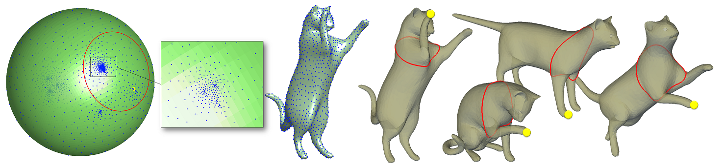
Figure 1. Sampling of the sphere-type cat surface (third from the left), and the sampling shown on the uniformization sphere (left). Note the zoom-in inset of the cat’s head. We also show the neighborhood (marked with red on the sphere) for $A=0.3$ of a point (marked with yellow ball on the sphere) on the cat’s front leg (the model is taken from the Non-rigid World data-set [5]). On the right we show the neighborhood corresponding to the yellow point on the original cat surface model (fourth from the right) and on few other surfaces from the same class (the neighborhoods were computed independently in each surface). Note the invariance of this neighborhood under nearly-isometric deformations.

4. Stability

In this section we prove Theorem 1.2; this is a first result connecting the new distance with local geodesic distortion. We will prove it for the disk case, but similar arguments can be used for the sphere case.

Proof.

(of Theorem 1.2) We will use three different metrics on $\mathcal{D}$: the metrics of $\mathcal{M},\mathcal{N}$ represented by the tensors $\widetilde{g},\widetilde{h}$ (resp.), and the hyperbolic metric $d_{H}(\cdot,\cdot)$.

The main idea of the proof is to use that a small value for $\mbox{\bf{d}}^{R}(\mathcal{M},\mathcal{N})$ means that there exists a $\pi\in\Pi(\mu,\nu)$ with respect to which the integral (1.2) of the cost function $d^{R}_{\mu,\nu}(z,w)$ is small as well; by the definition (1.9) of this cost function there must therefore be many corresponding neighborhoods $\Omega_{z_{0},R}$ and $\Omega_{w_{0},R}$ in $\mathcal{M}$ and $\mathcal{N}$ respectively that are very similar; we shall use these similarities to build local isometries.

Denote $\mbox{\bf{d}}^{R}(\mathcal{M},\mathcal{N})=\varepsilon$. Fix $K\subset\mathcal{D}$ to be a hyperbolic disk centered at the origin with an arbitrarily large (but finite) radius, $K=\Omega_{0,L}$. (Note: we could equally well have picked $K$ to be an arbitrary set that is compact in the hyperbolic metric; this particular choice alleviates notations.) Because $\Omega_{0,L+R}$ is a compact subset of $\mathcal{D}$, there exists a constant $C=C(L)<\infty$ such that $d_{H}(z,z^{\prime})\leq Cd_{g}(z,z^{\prime})$ for all $z,\,z^{\prime}\in\Omega_{0,L+R}$. Similarly, there exist positive constants $C^{\prime}=C^{\prime}(L),\,C_{1}=C_{1}(L)<\infty$ such that $\mu(z)\geq\frac{1}{C^{\prime}}$ for all $z\in\Omega_{0,L+R}$ and $\mbox{\rm{vol}}_{\mathcal{M}}(\Omega_{z,R/2})\geq\frac{2}{C_{1}}$ for all $z\in\Omega_{0,L}=K$ .

Now set $r<R/2C$. We will prove the desired bounds for arbitrary points $z_{1},z_{2}\in K$ such that $d_{g}(z_{1},z_{2})<r$. Let us pick such an arbitrary pair, which we shall keep fixed for the moment. We immediately note that $d_{H}(z_{1},z_{2})<R/2$.

Let now $\gamma_{z_{1},z_{2}}$ be the minimal-length-geodesic curve connecting $z_{1}$ and $z_{2}$ (in terms of the metric corresponding to surface $\mathcal{M}$); by taking $r>0$ sufficiently small we can ensure that this geodesic is unique. Since $d_{g}(z_{1},\xi)<r$ and thus $d_{H}(z_{1},\xi)<R/2$ for all $\xi\in\gamma_{z_{1},z_{2}}$, it follows that $\gamma_{z_{1},z_{2}}\subset\Omega_{z_{1},R/2}$. Morever, by a simple application of the triangle inequality, we have $\gamma_{z_{1},z_{2}}\subset\Omega_{z_{0},R}$ for all $z_{0}$ such that $d_{H}(z_{1},z_{0})<R/2)$, i.e. for all $z_{0}\in\Omega_{z_{1},R/2}$. It follows that

$$\Omega_{z_{1},R/2}\subset B:=\left\{z_{0}\ \mid\ \gamma_{z_{1},z_{2}}\subset\Omega_{z_{0},R}\right\}\,.$$

On the other hand, $\mbox{\rm{vol}}_{\mathcal{M}}(\Omega_{z_{1},R/2})\geq$ $\inf_{z\in K}\mbox{\rm{vol}}_{\mathcal{M}}(\Omega_{z,R/2})$ $=\min_{z\in K}\mbox{\rm{vol}}_{\mathcal{M}}(\Omega_{z,R/2})>\frac{2}{C_{1}}$. This implies that the volume of $B$ on the surface $\mathcal{M}$ can be bounded from below by

$$\mbox{\rm{vol}}_{\mathcal{M}}(B)\geq\mbox{\rm{vol}}_{\mathcal{M}}(\Omega_{z_{1},R/2})\geq\frac{2}{C_{1}}\,.$$

We can use this lower bound to show that there must be points $z_{0}$ in $B$, and corresponding points $w_{0}$ in $\mathcal{D}$, for which $d^{R}_{\mu,\nu}(z_{0},w_{0})$ is small. Indeed, let be $\pi^{*}$ an optimal transportation plan realizing the minimal transportation cost, then:

$$\varepsilon =\int_{\mathcal{D}\times\mathcal{D}}d^{R}_{\mu,\nu}(z,w)d\pi^{*}(z,w)\geq\int_{B\times\mathcal{D}}d^{R}_{\mu,\nu}(z,w)d\pi^{*}(z,w)$$

$$\geq\inf_{(z,w)\in B\times\mathcal{D}}\left[d^{R}_{\mu,\nu}(z,w)\right]\int_{B\times\mathcal{D}}d\pi^{*}(z,w)=\inf_{(z,w)\in B\times\mathcal{D}}\left[d^{R}_{\mu,\nu}(z,w)\right]\mbox{\rm{\footnotesize{vol}}}_{\mathcal{M}}(B).$$

There thus exists some point $(z_{0},w_{0})\in B\times\mathcal{D}$ such that

$$d^{R}_{\mu,\nu}(z_{0},w_{0})\leq\frac{2\,\varepsilon}{\mbox{\rm{\footnotesize{vol}}}_{\mathcal{M}}(B)}\leq C_{1}\,\varepsilon.$$

Next, we note that $d^{R}_{\mu,\nu}$ can be written as (see [19], and eq.(1.9))

$$d^{R}_{\mu,\nu}(z_{0},w_{0})=\inf_{m\in M_{\mathcal{D}},m(z_{0})=w_{0}}\int_{\Omega_{z_{0},R}}\left\|\widetilde{g}-m^{*}\widetilde{h}\right\|_{\widetilde{g}(z)}d\mbox{\rm{\footnotesize{vol}}}_{\mathcal{M}}(z)=\int_{\Omega_{z_{0},R}}\left|\mu(z)-\nu(m(z))\right|\,d\mbox{\rm{\footnotesize{vol}}}_{H}(z),$$

where $\|\cdot\|_{\widetilde{g}(z)}$ is the norm in the relevant tensor space as defined in Section 3 (and in [19]). The $m\in M_{\mathcal{D}}$ that satisfy $m(z_{0})=w_{0}$ constitute a one-parameter compact family, so that the infimum is achieved; let us call $f^{z_{0}}$ this minimizing Möbius transformation from $\Omega_{z_{0},R}$ to $\Omega_{w_{0},R}$. We have thus

$$\int_{\Omega_{z_{0},R}}\left\|\widetilde{g}-\left(f^{z_{0}}\right)^{*}\widetilde{h}\right\|_{\widetilde{g}(z)}d\mbox{\rm{\footnotesize{vol}}}_{\mathcal{M}}(z)=\int_{\Omega_{z_{0},R}}\left|\mu(z)-\nu(f^{z_{0}}(z))\right|\,d\mbox{\rm{\footnotesize{vol}}}_{H}(z)\leq C_{1}\,\epsilon\,.$$

Now

$$s(z)=\left|\mu(z)-\nu(f^{z_{0}}(z))\right|$$

is Lipschitz as a function of the argument $z$, since $\mu,\nu$ are Lipschitz on $\Omega_{0,L+2R}\subset\mathcal{D}$, and $f^{z_{0}}$ is analytic; moreover, by observing that $\Omega_{z_{0},R}\subset\Omega_{0,L+2R}$, we can bound the Lipschitz constant for $s$ independently of the particular choices made so far, i.e., for all $z,\,z^{\prime}\in\Omega_{z_{0},R}$,

$$|s(z)-s(z^{\prime})|\leq\kappa\,|z-z^{\prime}|\,.$$

Take now any $u$ in $\Omega_{z_{0},R}$, and set $S=s(u)$. Then

$$C_{1}\,\epsilon\geq\int_{\Omega_{z_{0},R}}\max(0,S-\kappa|u-z|)\,d\mbox{\rm{\footnotesize{vol}}}_{H}(z)\geq C^{\prime\prime}\,S^{3}\,,$$

where $C^{\prime\prime}>0$ can be picked independently of the location of $u$ within $\Omega_{z_{0},R}$, and uniformly for $z_{0}\in\Omega_{0,L+R}$. It follows that $S\leq C_{2}\,\epsilon^{1/3}$. This shows that

(4.1) $$\max_{z\in\Omega_{z_{0},R}}\left\|\widetilde{g}-m^{*}\widetilde{h}\right\|_{\widetilde{g}(z)}\leq C_{2}\,\varepsilon^{1/3}\,,$$

for some constant $C_{2}$ that doesn’t depend on $\epsilon$ or $z_{1},\,z_{2}$.

Given arbitrary $z_{1}$, $z_{2}$ in $K$, we have thus found $\Omega_{z_{0},R}$ that contains the full geodesic $\gamma_{z_{1},z_{2}}$ and a Möbius map $f^{z_{0}}$ from $\Omega_{z_{0},R}$ to a corresponding $\Omega_{w_{0},R}$ that, within to a small error controlled by the small quantity $\mbox{\bf{d}}^{R}(\mathcal{M},\mathcal{N})$, maps the local geometry in $\mathcal{M}$ to that in $\mathcal{N}$.

To alleviate notations in what follows, we drop the superscript $z_{0}$ on $f^{z_{0}}$. Our plan is to use the minimizing geodesic path $\gamma_{z_{1},z_{2}}(t):[0,1]\rightarrow\mathcal{M}$ between the points $\gamma_{z_{1},z_{2}}(0)=z_{1}$, and $\gamma_{z_{1},z_{2}}(1)=z_{2}$ to compute bounds on $d_{h}(f(z_{1}),f(z_{2}))$. Using the differential $[Df]$ of the map $f$, which is a linear map between the tangent spaces $T_{z}\mathcal{M}$ (with the metric $\widetilde{g}$) and $T_{w}\mathcal{N}$ (with the metric $\widetilde{h}$), we have

$$d_{h}(f(z_{1}),f(z_{2})) \leq\int_{0}^{1}\left\|\frac{d}{dt}f(\gamma_{z_{1},z_{2}}(t))\right\|_{h}dt$$

$$\leq\int_{0}^{1}\left\|[Df]\right\|\left\|\dot{\gamma}_{z_{1},z_{2}}(t)\right\|_{g}dt$$

(4.2) $$\leq\max_{z\in\gamma_{z_{1},z_{2}}}\left\|[Df(z)]\right\|d_{g}(z_{1},z_{2})\,,$$

which shows that an upper bound on $\max_{z\in\gamma_{z_{1},z_{2}}}\left\|[Df(z)]\right\|$ will give us one of the desired inequalities.

The second inequality is achieved using that

$$d_{g}(f^{-1}(f(z_{1})),f^{-1}(f(z_{2}))) =\int_{0}^{1}\left\|\frac{d}{dt}f^{-1}(\gamma_{f(z_{1}),f(z_{2})}(t))\right\|_{g}dt$$

$$\leq\int_{0}^{1}\left\|[Df^{-1}]\right\|\left\|\dot{\gamma}_{f(z_{1}),f(z_{2})}(t)\right\|_{h}dt$$

(4.3) $$\leq\max_{w\in\gamma_{f(z_{1}),f(z_{2})}}\left\|[Df(w)]^{-1}\right\|d_{h}(f(z_{1}),f(z_{2})).$$

To use this, we thus need to upper bound $\max_{w\in\gamma_{f(z_{1}),f(z_{2})}}\left\|[Df(w)]^{-1}\right\|$.

In the remainder of this proof, we show how bounds on $\max_{z\in\gamma_{z_{1},z_{2}}}\left\|[Df(z)]\right\|$ and $\max_{w\in\gamma_{f(z_{1}),f(z_{2})}}\left\|[Df(w)]^{-1}\right\|$ can be derived from (4.1).

First, we take an orthonormal basis $E=\left\{e_{1},e_{2}\right\}\subset T_{z}\mathcal{M}$. That is,

(4.4) $$e_{k}^{i}e_{\ell}^{j}g_{ij}=e_{k}^{i}e_{\ell}^{j}\widetilde{\mu}(z)\delta_{i,j}=\delta_{k,\ell}.$$

Similarly we take orthonormal basis $B=\left\{b_{1},b_{2}\right\}\subset T_{w}\mathcal{N}$.

We will denote the matrix $[Df]=[Df_{z}]$ representing the differential $Df_{z}$ of $f$ at the point $z$, in the bases $E,B$. The norm of $Df_{z}$ is the induced norm

$$\left\|Df_{z}\right\|=\max_{\xi\in T_{z}\mathcal{M},\xi\neq 0}\frac{\left\|Df(\xi)\right\|_{\widetilde{h}(f(z))}}{\left\|\xi\right\|_{\widetilde{g}(z)}}.$$

Writing the tensor $\widetilde{g}$ in the basis $E$ we get the Euclidean form $\widetilde{g}(z)=de_{1}\otimes de_{1}+de_{2}\otimes de_{2}$, and the tensor $\widetilde{h}$ in the basis $B$ will have the same form $\widetilde{h}(w)=db_{1}\otimes db_{1}+db_{1}\otimes db_{2}$. The pull-back $f^{*}\widetilde{h}(z)$ will have the form $f^{*}\widetilde{h}(z)=\left([Df_{z}]^{t}[Df_{z}]\right)_{ij}de_{i}\otimes de_{j}$. Therefore in the basis $E$ we have

$$\left\|\widetilde{g}-f^{*}\widetilde{h}\right\|_{\widetilde{g}(z)}=\left\|Id-[Df]^{t}[Df]\right\|_{F},$$

where $Id$ is the $2\times 2$ identity matrix, and $\left\|\cdot\right\|_{F}$ denotes the Frobenius norm.

Writing the singular value decomposition of $[Df]$ we have

$$[Df]=Q\,\mbox{diag}\left(\sigma_{1}(z),\sigma_{2}(z)\right)R^{T},$$

where $Q,R$ are orthogonal and $\sigma_{1}\leq\sigma_{2}$ are the respective singular values. Then we have

(4.5) $$\left\|\widetilde{\mu}-f^{*}\widetilde{\nu}\right\|_{g(z)}^{2}=\left\|Id-[Df]^{T}[Df]\right\|^{2}_{F}=\left\|R\left(Id-\left(\begin{array}[]{cc}(\sigma_{1}(z))^{2}&0\\ 0&(\sigma_{2}(z))^{2}\\ \end{array}\right)\right)R^{T}\right\|^{2}_{F}=(1-\sigma_{1}(z)^{2})^{2}+(1-\sigma_{2}(z)^{2})^{2},$$

Using (4.1),(4.5) we get

$$\left|1-\sigma_{2}(z)^{2}\right|\leq C_{2}\varepsilon^{1/3}.$$

From this last bound on $\sigma_{2}(z)$ for $z\in\Omega_{z_{0},R}$ there exists a constant $C_{3}>0$ such that

$$0\leq\sigma_{2}(z)\leq 1+C_{3}\varepsilon^{1/3}.$$

Since $\left\|[Df]\right\|=\sigma_{2}$, this is the desired estimate for the first inequality.

For the second inequality, we need to bound $\left\|[Df]^{-1}\right\|=\sigma_{1}^{-1}$. The computation (4.5) shows that

$$\left|1-\sigma_{1}(z)^{2}\right|\leq C_{2}\varepsilon^{1/3}\,,$$

from which we obtain

$$0\leq\frac{1}{\sigma_{1}(z)}\leq 1+C_{4}\varepsilon^{1/3}\,,$$

which concludes our argument.

∎

5. Experimental validation and comments

In this section we perform experimental validation of our algorithms. We have tested and experimented with our algorithms on four different data-sets:

1. Non-rigid World data-set [5]. This data-set was distributed by Bronstein,Bronstein and Kimmel and was specifically constructed for evaluating shape comparison algorithms in the scenario of non-rigid shapes; it contains meshes of different objects (cats, dogs, wolves, humans, etc…) in different poses. We compare our results on this data-set to the Gromov-Hausdorff algorithm suggested in [1, 5].

2. SHREC 2007 Watertight Benchmark [10] This data-set contains meshes of several objects within a given semantic class for several different classes, such as chairs, 4-legged animals, humans, etc… It is more challenging for isometric-invariant matching algorithms since most of the objects are far from isometric to the objects in the same semantic class, for example the 4-legged animals class contains a giraffe and a dog.

3. Synthetic. We constructed this data-set to test the effect of the “size” parameter $R$ on the distance behavior.

4. Primate molar teeth. This data-set originates from a real biological problem/application; it consists of molar teeth surface for different primates. It was communicated to us by biologists who compare these shapes for characterization and classification of mammals.

Remark 5.1.

For all data-sets, we scaled the meshes to have unit area, because our goal is to compare surfaces solely based on shape, regardless of size.

Non-rigid World data-set and comparison to Gromov-Hausdorff-type distance. In the first experiment we ran our sphere-type algorithm to determine conformal Wasserstein distances for all pairs in the Non-rigid World data-set, distributed by Bronstein, Bronstein and Kimmel [1, 5, 4]; we compare the results to those obtained using the code for the (symmetrized) partial embedding Gromov-Hausdorff (speGH) distance distributed by the same authors. The speGH distance has been used with great success in surface comparison [1, 5, 4] and can handle situations beyond the scope of our, more limited algorithm, it can e.g., compare surfaces of different genus. We therefore consider it as a state-of-the-art algorithm. In order to compare our Conformal Wasserstein distance with speGH for applications of interest to us, we use both algorithms on Non-rigid World data-set where all the surfaces are scaled to have unit area and where 100 sample points are chosen on each surface.

The Non-rigid World data-set contains meshes of different poses of the following articulated objects: a centaur, a cat, a dog, a horse, a human female, and two human males (“Michael” and “David”).

The two resulting dissimilarity matrices are shown in Figure 2 (a,d). The dissimilarity matrices are both normalized by translating the minimal value to zero and scaling the maximal value to one. The color scheme is Matlab’s “Jet” where dark blue represents low (close to zero) value, and dark red indicates high (close to one) values. The Sphere-type algorithm used $A=0.3$, and a $30\times 30$ bins discretization with the convolution kernel $(1,1,1)\otimes(1,1,1)$ (all the sphere-type examples use these bin settings) to obtain the discretizations of the conformal density. The timing for running one comparison $\mbox{\bf{d}}^{A}(\mathcal{M},\mathcal{N})$ was 90 seconds on 2.2GHz AMD Opteron processor. Figure 2 (b-c) and (e-f) shows two nearest neighbors classifications tests where a white square inside a dark-red area means success and white square on black area is a failure.

The structure of the dissimilarity matrix is illustrated in the two plots in Figure 3. Figure 3 (a) shows the classification rates as a function of the number $K$ of nearest neighbors, where for each fixed $K$ we calculated the classification rate as follows. For each object we counted how many from its $K$-nearest neighbors are of the same class. We summed all these numbers and divided by the total number of possible correct classifications. The blue curve shows the analysis of the dissimilarity matrix output by our distance algorithm and the red curve by the speGH distance code. In (b) we show the ROC curve where for every $K=1,2,..,10$ we plot the True Positive Rate (TPR), that is the number of true positives divided by the number of positives, as a function of the False Positive Rate (FPR), that is the number of false positives divided by the number of negatives.

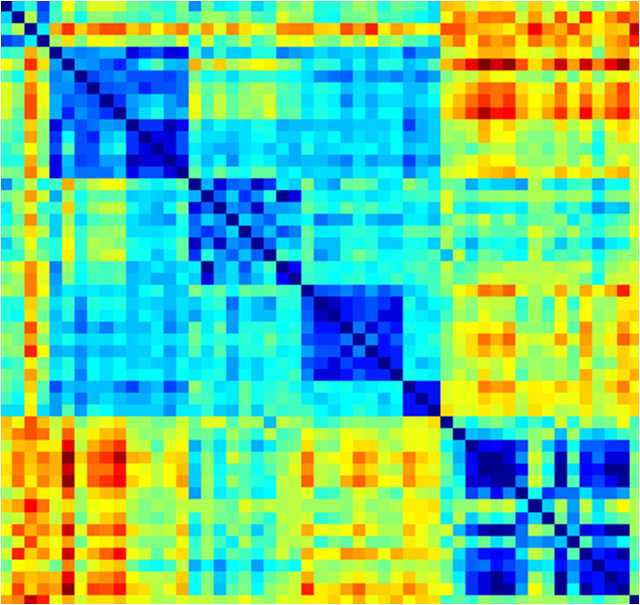
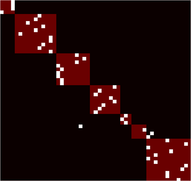
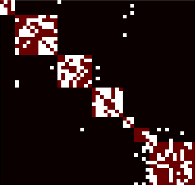
(a) This paper’s dissimilarity matrix	(b) $1^{st}$ nearest neighbor	(c) $5$ nearest neighbors
	$94\%$ classification rate	$87\%$ classification rate
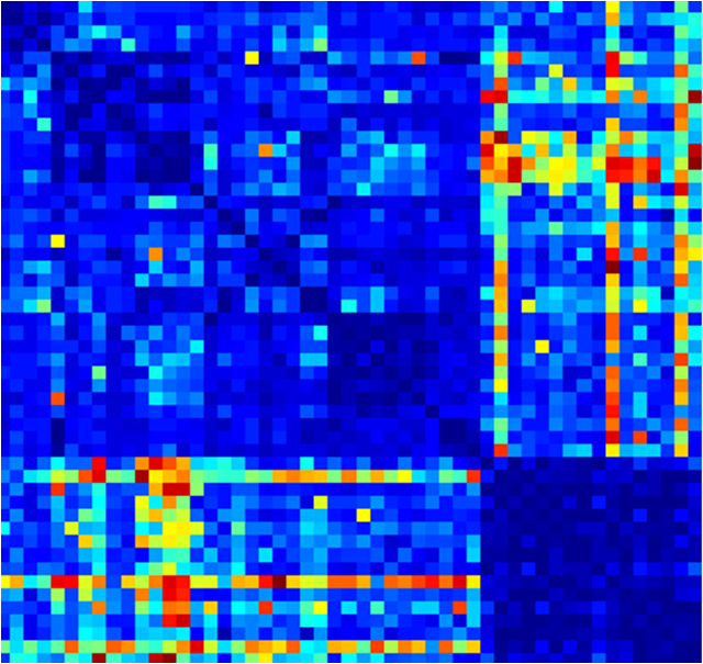
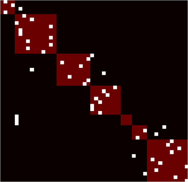
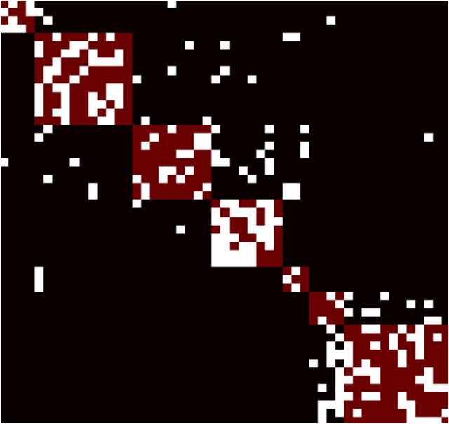
(d) speGH dissimilarity matrix	(e) $1^{st}$ nearest neighbor	(f) $5$ nearest neighbors
	$78\%$ classification rate	$68\%$ classification rate

Figure 2. The dissimilarity matrices for the unit area scaled Non-rigid World data-set [1, 5] calculated with the conformal Wasserstein (CW) distance given by our algorithm (a) and the symmetric partial-embedding Gromov-Hausdorff (speGH) distance [1, 5] (d). In the second column (b,e) we show the ground truth classification matrix (dark-red) and the first nearest neighbor (white) according to the CW (in b) and to the speGH (in e) distance for each row. The third column (c,f) shows the five nearest neighbors (when there are fewer than five in some category we simply limit ourselves to the number in that category). Note that white squares should be in dark red regions to indicate correct classification. Note that with only 100 sampling points, “Michael” and “David” are not distinguishable, so if a pose of Michael is among the nearest neighbors of a pose of David, we still count it as a correct classification.

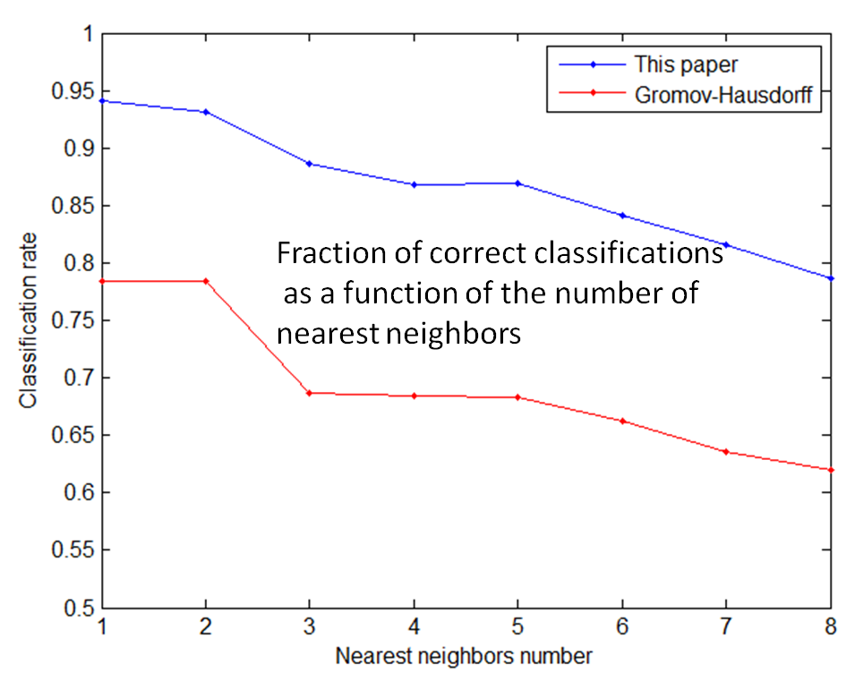
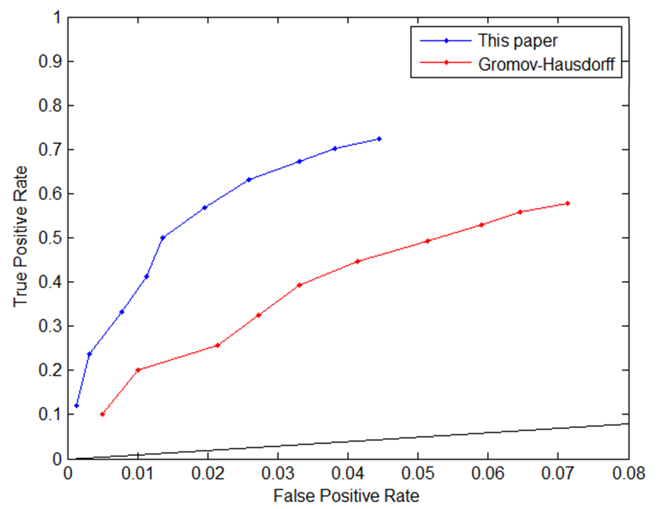
(a) Correct Classification Rate	(b) ROC curve (TPR/FPR)

Figure 3. Correct Classification Rate and ROC curves for the dissimilarity matrices produces by our method (blue) and Gromov-Hausdorff-type metric (red). See text for details.

SHREC 2007 Watertight Benchmark [10]. Our next experiment deals with a data-set with larger in-class variations; SHREC 2007 contains 20 categories of models with 20 meshes for each category (400 meshes in total) the categories are, e.g., chairs, 4-legged animals, humans, planes, tables, etc…

For our experiment, we restricted ourselves to all the meshes of 8 categories that contained only surfaces of genus zero (since our current algorithm does not support surfaces of higher genus) and that seemed intrinsically similar; these categories were: humans, 4-legged animals, ants, hands, airplanes, teddy-bears, pliers, Armadillos. We ran our sphere-type algorithm to compute the distance between all pairs. We tested the “size” parameters $A=0.3,0.4,0.5$. The bin was the same as for the previous data-set. However, to achieve faster running times (we had about 25,000 comparisons…) we took only $50$ sample points. The running time for one pair of objects was around $15$ seconds.

Figure 4 shows the dissimilarity matrices (top row) using the three different values if $A$: $0.3,0.4,0.5$, and the dissimilarity matrix resulting from combining them:

$$T_{d}(\mu,\nu)=T_{d}^{0.3}(\mu,\nu)\cdot T_{d}^{0.4}(\mu,\nu)\cdot T_{d}^{0.5}(\mu,\nu).$$

Note that $T_{d}(\mu,\nu)$ is also a metric and suggests a way to remove the influence of the size parameter if desired. The combined distance produced the best classification results as seen in the bottom row, where for each row the white square shows the nearest neighbor to that object. The dark red areas represent the different categories. The combined distance reached the very high classification rate of $95\%$ on this challenging data-set. Figure 5 shows for one object in each category its four closest neighbors. Note the non-rigid nature of some of the objects (e.g., humans, hands), and the substantial deviation from perfect isometry within class (e.g., 4-legged animals). Figure 6 demonstrates a partial failure case where although the first two nearest neighbors to the Giraffe are within the 4-legged animals category, the third nearest neighbor is the one-armed armadillo, which belong to a different category (remember that the algorithm is size invariant).

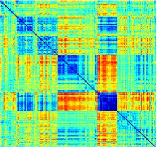
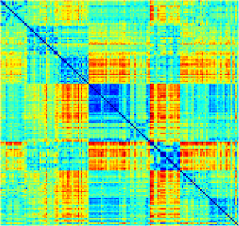
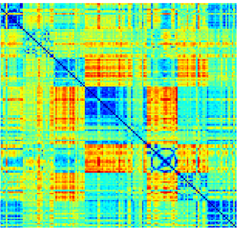
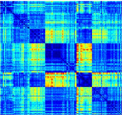
$R=0.3$	$R=0.4$	$R=0.5$	combined $R=0.3,0.4,0.5$
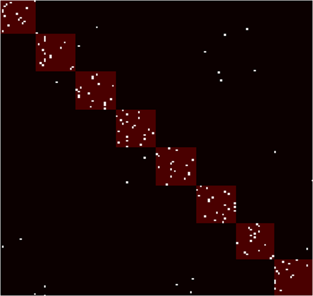
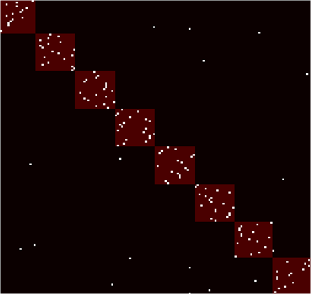
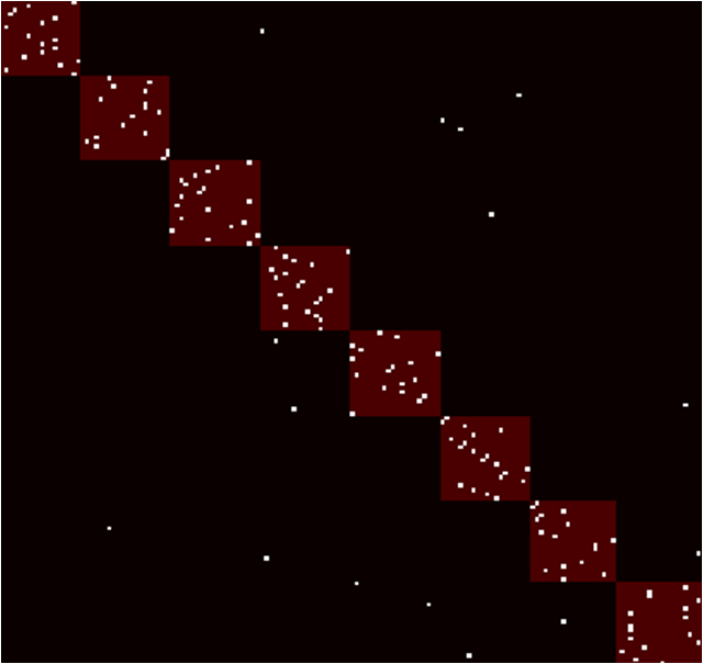
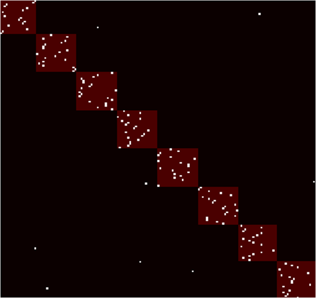
classification rate: $85\%$	$89\%$	$90\%$	$95\%$

Figure 4. Dissimilarity matrices (top row) for the SHREC 2007 watertight Benchmark [10] with different size parameter: $R=0.3,0.4,0.5$ and their combination (see text for details). Bottom row shows the first nearest neighbor classification test where white squares denote the nearest neighbor of that row’s object and the dark red area represent correct category classification.

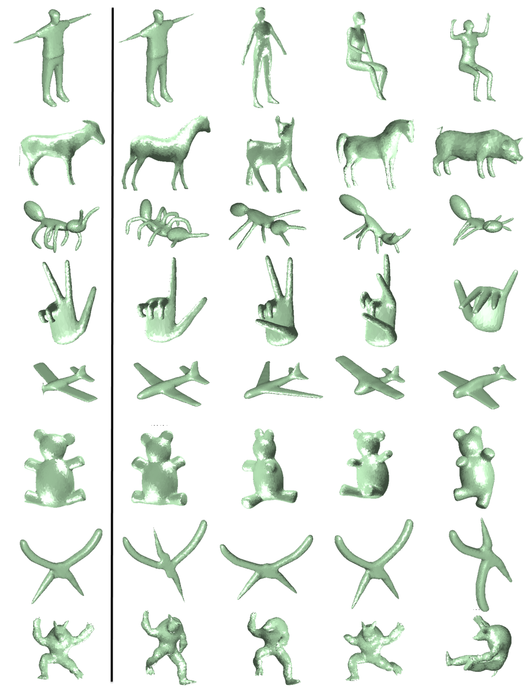
Figure 5. SHREC 2007 watertight Benchmark [10]: we show the four closest neighbors to each of the objects on the left side (we show one example from each category).

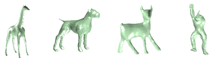
Figure 6. SHREC 2007 watertight Benchmark [10]: a partially failure case where the giraffe has correct two nearest neighbors, however its $3^{rd}$ nearest neighbor is a one armed armadillo. Remember that our matching is scale invariant.

Synthetic data-set. This experiment was designed to test the influence of the size parameter $R$ on the behavior of the distance. The surfaces we compared are shown in the top row of Figure 7, they each have three small bumps, in different positions. At first sight, one might think that for small $R$, the distance $\mbox{\bf{d}}^{R}(\mathcal{M},\mathcal{N})$ based on comparing neighborhoods of “size” $R$, would have trouble distinguishing these objects from each other. However, one should keep in mind that the uniformization process is a global one: changing the metric in one region of the surface would effect the uniformization of other regions (but influence would decay like appropriate Green’s function). Figure 7 plot the distance of disk-type model $A$ to the four others, for different $R$ values. We also show hyperbolic neighborhoods corresponding to the three different size parameters (color coded the same way as the graphs). We scaled the distances to have maximum of one (since smaller $R$ results naturally in smaller distances). Note that even the smallest size value $R=0.25$ already distinguishes between the different models. Further note, that larger size parameters such as $R=0.75$ results in slightly more intuitive linear distance behavior. Overall, the size parameter $R$ does affect the distance, but not in a very significant way.

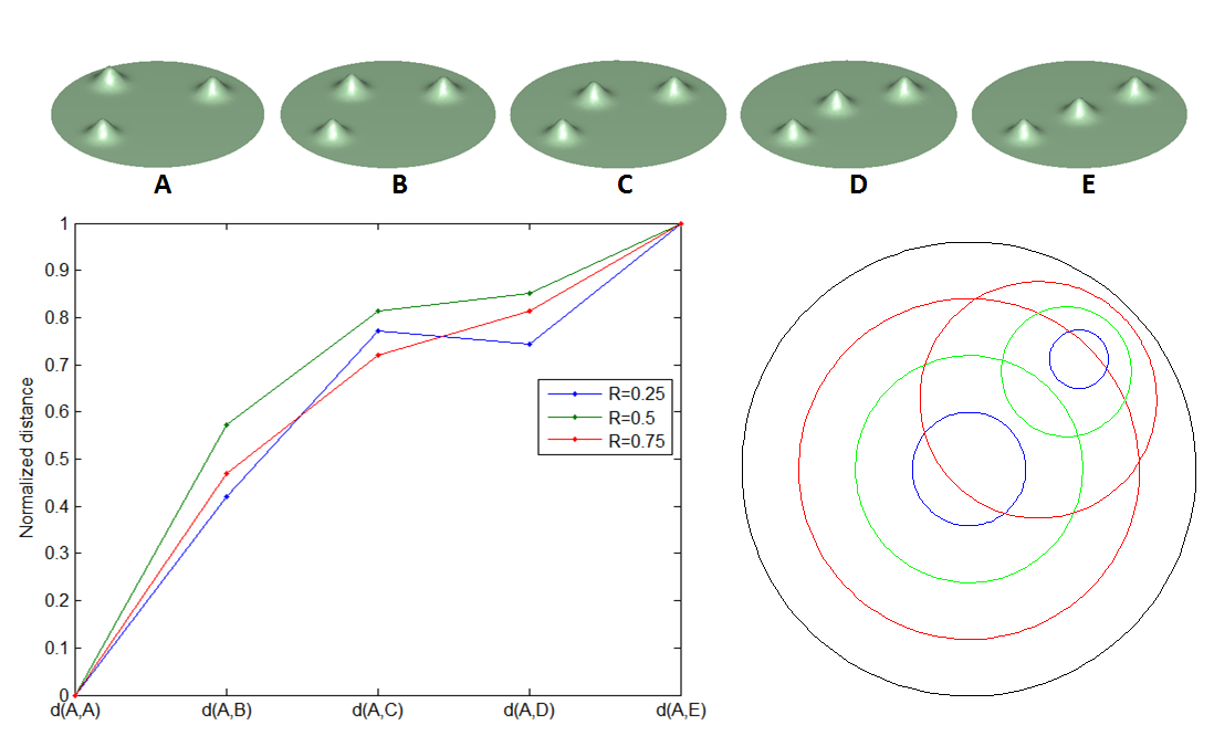
Figure 7. Testing influence of the size parameter $R$ to sperate identical models with small features. We compare the distances of the disk model marked with $A$ to all other models $A-E$ using three different size parameters $R=0.25,0.5,0.75$. We also show examples of hyperbolic disk of these radii as used by our disk-type algorithm (the are color coded like the graph lines).

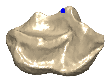
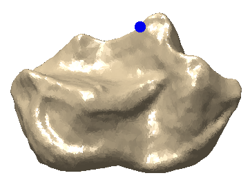
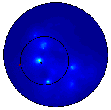
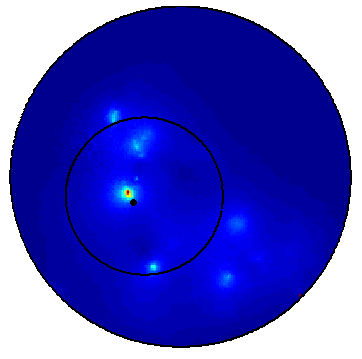
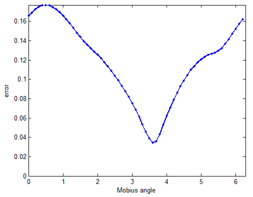
(a)				Good pair (a)
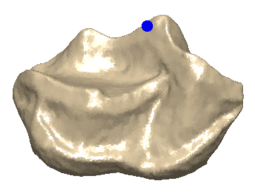
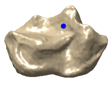
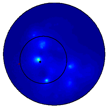
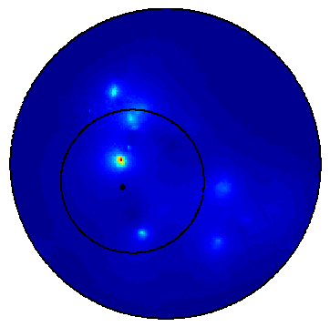
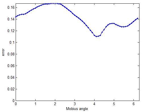
(b)				Erroneous pair (b)

Figure 8. Calculation of the local distance $d^{R}_{\mu,\nu}(\cdot,\cdot)$ between pairs of points on two different surfaces (each row shows a different pair of points; the two surfaces are the same in the top and bottom rows). The first row shows a “good” pair of points together with the alignment of the conformal densities $\mu,m^{*}\nu$ based on the best Möbius transformation $m$ minimizing $d^{R}_{\mu,\nu}$. The plot of this latter integral as a function of $m$ (parameterized by $\sigma\in[0,2\pi)$, see (1.5)) is shown in the right-most column. The second row shows a “bad” correspondence which indeed leads to a higher local distance $d^{R}_{\mu,\nu}$.

Primate molar teeth. Finally, we present a few experimental results related to a biological application; in a case study of the use of our approach to the characterization of mammals by the surfaces of their molars, we compare high resolution scans of the masticating surfaces of molars of several lemurs, which are small primates living in Madagascar. Traditionally, biologists specializing in this area carefully determine landmarks on the tooth surfaces, and measure characteristic distances and angles involving these landmarks. A first stage of comparing different tooth surfaces is to identify correspondences between landmarks. Figure 8 illustrates how $d^{R}_{\mu,\nu}(z,w)$ (disk-type) can be used to find corresponding pairs of points on two surfaces by showing both a “good” and a “bad” corresponding pair. The left two columns of the figure show the pair of points in each case; the two middle columns show the best fit after applying the minimizing Möbius on the corresponding disk representations; the rightmost column plots $\int_{\Omega_{z_{0},R}}\,|\,\mu(z)-(m_{z_{0},w_{0},\sigma}^{*}\nu)(z)\,|\,d\mbox{\rm{\footnotesize{vol}}}_{H}(z)$, the value of the “error”, as a function of parameter $\sigma$, parameterizing the Möbius transformations that map a given point $z_{0}$ to another given point $w_{0}$ (they are parameterized over $S^{1}$, see Lemma 3.5 in [19] ). The “best” corresponding point $w_{0}$ for a given $z_{0}$ is the one that produces the lowest minimal value for the error, i.e. the lowest $d^{R}_{\mu,\nu}(z_{0},w_{0})$.

Figure 9 show the top 120 most consistent corresponding pairs (in groups of 20) for two molars belonging to lemurs of different species. Corresponding pairs are indicated by highlighted points of the same color. These correspondences have surprised the biologists from whom we obtained the data sets; their experimental measuring work, which incorporates finely balanced judgment calls, had defied earlier automatization attempts.

Once the differences and similarities between molars from different animals have been quantified, they can be used (as part of an approach) to classify the different individuals. Figure 10 illustrates a preliminary result that illustrates the possibility of such classifications based on the distance operator between surfaces introduced in this paper. The figure illustrates the pairwise distance matrix for eight molars, coming from individuals in four different species (indicated by color). The clustering was based on only the distances between the molar surfaces; it clearly agrees with the clustering by species, as communicated to us by the biologists from whom we obtained the data sets.

One final comment regarding the computational complexity of our method. There are two main parts: the preparation of the distance matrix $d_{ij}$ and the linear programming optimization. For the linear programming part we used a Matlab interior point implementation with $N^{2}$ unknowns, where $N$ is the number of points spread on the surfaces. In our experiments, the optimization typically terminated after $15-20$ iterations for $N=150-200$ points, which took about 2-3 seconds. The computation of the similarity distance $d_{ij}$ took longer, and was the bottleneck in our experiments. We separate the disk-type and the sphere-type algorithms.

For the sphere-type algorithm if we use $N=\mathcal{L}$ sample points ($Q$) on each surface (see Section 3) then for each pair we compare the difference (using fixed size bin structure) of the discrete conformal densities for fixed number of Möbius transformations. This results in $O(N^{3})$ algorithm for computing the distance matrix $d_{ij}$. In our experiments the total distance computation time (including linear programming optimization) was around $15$ seconds for $N=\mathcal{L}=50$ (in the SHREC 2007 data-set), to $90$ second per comparison for $N=\mathcal{L}=100$ (in the Non-rigid world data-set). In the sphere-type examples we have used 2.2GHz AMD Opteron processor. The sphere-type algorithm was coded completely in Matlab and was not optimized.

For the disk-type algorithm, if we spread $N$ points on each surface, and use them all to interpolate the conformal factors $\Gamma_{\mu},\Gamma_{\nu}$, if we use $P$ points in the integration rule, and take $L$ points in the Möbius discretization (see Section 2 for details) then each approximation of $d^{R}_{\mu,\nu}(z_{i},w_{j})$ by (2.5) requires $O(L\cdot P\cdot N)$ calculations, as each evaluation of $\Gamma_{\mu},\Gamma_{\nu}$ (Thin-Plate Spline approximation we use to interpolate the conformal densities, described in Appendix B) takes $O(N)$ and we need $L\cdot P$ of those. Since we have $O(N^{2})$ distances to compute, the computation complexity for calculating the similarity distance matrix $d_{ij}$ is $O(L\cdot P\cdot N^{3})$. This step was coded in C++ (and therefore the time difference to the sphere-type case) and took $3.5$ seconds for $N=50$, $51$ seconds for $N=100$, under $5$ minutes for $N=150$ and two hours for $N=300$ (in these examples we took $P\approx N$). However, also in this case we have not optimized the algorithm and we believe these times can be reduced significantly. The disk-type algorithm ran on Intel Xeon (X5650) 2.67GHz processor.

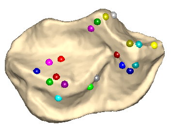
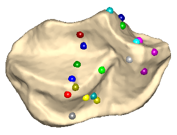
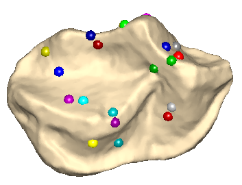
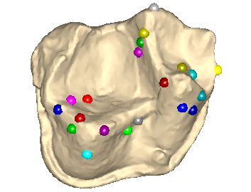
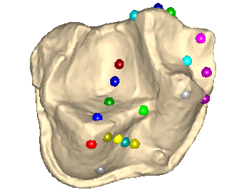
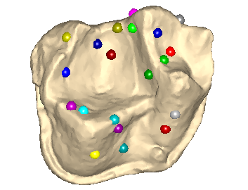
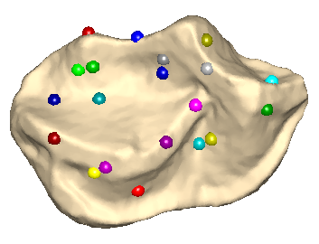
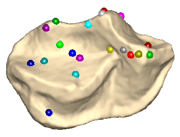
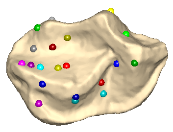
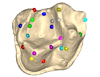
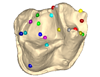
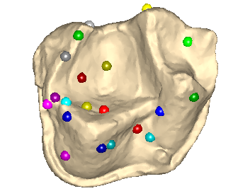
Figure 9. The top 120 most consistent corresponding pairs between two molar teeth models.

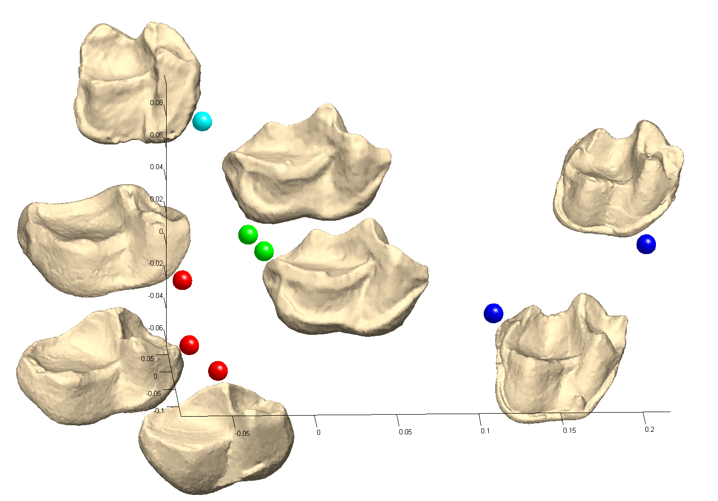
Figure 10. Embedding of the distance graph of eight teeth models using multi-dimensional scaling. Different colors represent different lemur species. The graph suggests that the geometry of the teeth might suffice to classify species.

6. Acknowledgments

The authors would like to thank Cédric Villani and Thomas Funkhouser for valuable discussions. We are grateful to Jukka Jernvall, Stephen King, and Doug Boyer for providing us with the tooth data sets, and for many interesting comments. We would like to thank the anonymous reviewers that challenged us to improve our manuscript with excellent comments and suggestions. ID gratefully acknowledges (partial) support for this work by NSF grant DMS-0914892, and by an AFOSR Complex Networks grant; YL thanks the Rothschild foundation for postdoctoral fellowship support.

Appendix A

We prove Theorem 2.1. We start with a simple lemma showing that all Möbius transformations restricted to $\Omega_{0,T}$, $T<\infty$, are Lipschitz with a universal constant, for which we provide an upper bound.

Lemma A.1.

A Möbius transformation $m\in M_{\mathcal{D}}$ restricted to $\Omega_{0,T}$, $T<\infty$ is Lipschitz continuous with Lipschitz constant $C_{m}\leq\frac{1-|a|^{2}}{(1-r_{T}|a|)^{2}}$, where $a=m^{-1}(0)$ and $r_{T}=tanh(T)$.

Proof.

Denote $m(z)=e^{\textbf{\footnotesize{i}}\theta}\frac{z-a}{1-z\overline{a}}$. Then, for $z,w\in\Omega_{0,T}$ we have

$$\Big{|}m(z)-m(w)\Big{|} \leq\Big{|}e^{\textbf{\footnotesize{i}}\theta}\frac{z-a}{1-z\overline{a}}-e^{\textbf{\footnotesize{i}}\theta}\frac{w-a}{1-w\overline{a}}\Big{|}\leq\Big{|}\frac{(z-a)(1-w\overline{a})-(w-a)(1-z\overline{a})}{(1-z\overline{a})(1-w\overline{a})}\Big{|}$$

$$\leq\Big{|}\frac{(z-w)(1-\left|a\right|^{2})}{(1-z\overline{a})(1-w\overline{a})}\Big{|}\leq|z-w|\frac{1-\left|a\right|^{2}}{(1-r_{T}\left|a\right|)^{2}}.$$

∎

Next we prove:
Theorem 2.1 For Lipschitz continuous $\mu,\nu$,

$$\left|\,d^{R}_{\mu,\nu}(z_{i},w_{j})-\min_{m(z_{i})=w_{j}}\sum_{k}\,\alpha_{k}\,\left|\,\mu(\widetilde{m}_{i}(p_{k}))-\nu(m(\widetilde{m}_{i}(p_{k})))\,\right|\,\right|\leq C\,\varphi_{E}\left(\left\{p_{k}\right\}\right)~{},$$

where the constant $C$ depends only on $\mu,\nu,R$.

Proof.

First, denote $f(z)=\Big{|}\mu(\widetilde{m}_{i}(z))-\nu(m(\widetilde{m}_{i}(z)))\Big{|}$. Then,

$$\Big{|}\int_{\Omega_{0,R}}f(z)d\mbox{\rm{\footnotesize{vol}}}_{H}(z)-\min_{m(z_{i})=w_{j}}\sum_{k}\alpha_{k}f(p_{k})\Big{|} \leq\sum_{k}\int_{\Delta_{k}}\Big{|}f(z)-f(p_{k})\Big{|}d\mbox{\rm{\footnotesize{vol}}}_{H}(z)$$

$$\leq\omega^{\Omega_{0,R}}_{f}\left(\varphi_{E}\left(\left\{p_{k}\right\}\right)\right)\int_{\Omega_{0,R}}d\mbox{\rm{\footnotesize{vol}}}_{H},$$

where $\Delta_{k}$ are the intersections of $\Omega_{0,R}$ with the Euclidean Voronoi cells defined by the centers $p_{k}$, and the modulus of continuity $\omega^{\Omega_{0,R}}_{f}\left(h\right)=\sup_{|z-w|<h;z,w\in\Omega_{0,R}}\left|f(z)-f(w)\right|$ is used. Note that

(A.2) $$\omega^{\Omega_{0,R}}_{f}\leq\omega^{\Omega_{0,R}}_{\mu\circ\widetilde{m}_{i}}+\omega^{\Omega_{0,R}}_{\nu\circ m\circ\widetilde{m}_{i}}.$$

Denote the Lipschitz constants of $\mu,\nu$ by $C_{\mu},C_{\nu}$, respectively. From Lemma A.1 we see that, for $z,w\in\Omega_{0,R}$,

$$\Big{|}\mu(\widetilde{m}_{i}(z))-\mu(\widetilde{m}_{i}(w))\Big{|} \leq C_{\mu}\Big{|}\widetilde{m}_{i}(z)-\widetilde{m}_{i}(w)\Big{|}\leq C_{\mu}\frac{1-|a|^{2}}{(1-r_{R}|a|)^{2}}\left|z-w\right|\leq C_{\mu}\frac{1}{(1-r_{R})^{2}}\left|z-w\right|,$$

which is independent of $\widetilde{m}_{i}$. Similarly,

$$\Big{|}\nu(m(\widetilde{m}_{i}(z)))-\nu(m(\widetilde{m}_{i}(w)))\Big{|} \leq C_{\nu}\Big{|}m(\widetilde{m}_{i}(z))-m(\widetilde{m}_{i}(w))\Big{|}\leq C_{\nu}\frac{1}{(1-r_{R})^{2}}\left|z-w\right|,$$

which is independent of $m,\widetilde{m}_{i}$. Combining these with eq. (A-A.2) we get

$$\Big{|}\int_{\Omega_{0,R}}f(z)d\mbox{\rm{\footnotesize{vol}}}_{H}(z)-\min_{m(z_{i})=w_{j}}\sum_{k}\alpha_{k}f(p_{k})\Big{|}\leq\left(C_{\mu}+C_{\nu}\right)\frac{\int_{\Omega_{0,R}}d\mbox{\rm{\footnotesize{vol}}}_{H}}{(1-r_{R})^{2}}\varphi_{E}\left(\left\{p_{k}\right\}\right),$$

which finishes the proof. ∎

Finally, we prove:

Theorem 2.2 For Lipschitz continuous $\mu,\nu$,

$$\left|\,d^{R}_{\mu,\nu}(z_{i},w_{j})-\breve{d}^{R}_{\mu,\nu}(z_{i},w_{j})\right|\leq C_{1}\,\varphi_{E}\left(\left\{p_{k}\right\}\right)+C_{2}\,L^{-1}~{},$$

where the constants $C_{1},C_{2}$ depend only on $\mu,\nu,R$.

Proof.

In view of Theorem 2.1 it is sufficient to prove that

$$\left|\widehat{d}^{R}_{\mu,\nu}(z_{i},w_{j})-\breve{d}^{R}_{\mu,\nu}(z_{i},w_{j})\right|\leq C\,L^{-1},$$

for an appropriate constant $C$ depending only upon $\mu,\nu,R$. Denote by $m_{i,j}$ the minimizer of $\widehat{d}^{R}_{\mu,\nu}(z_{i},w_{j})$. Then

$$\left|\widehat{d}^{r}_{\mu,\nu}(z_{i},w_{j})-\breve{d}^{r}_{\mu,\nu}(z_{i},w_{j})\right| =\mathop{\min}_{\ell=1..L}\left|\sum_{k}\alpha_{k}\Big{[}\left|\mu(\widetilde{m}_{i}(p_{k}))-\nu(m_{i,j}(\widetilde{m}_{i}(p_{k})))\right|-\left|\mu(\widetilde{m}_{i}(p_{k}))-\nu(m_{z_{i},w_{j},2\pi\ell/L}(\widetilde{m}_{i}(p_{k})))\right|\Big{]}\right|$$

$$\leq\mathop{\min}_{\ell=1..L}\sum_{k}\alpha_{k}\Big{|}\nu(m_{i,j}(\widetilde{m}_{i}(p_{k})))-\nu(m_{z_{i},w_{j},2\pi\ell/L}(\widetilde{m}_{i}(p_{k})))\Big{|}$$

$$\leq C_{\nu}\mathop{\min}_{\ell=1..L}\sum_{k}\alpha_{k}\Big{|}m_{i,j}(\widetilde{m}_{i}(p_{k}))-m_{z_{i},w_{j},2\pi\ell/L}(\widetilde{m}_{i}(p_{k}))\Big{|}$$

$$\leq\frac{C_{\nu}}{(1-r_{R})^{2}}\mathop{\min}_{\ell=1..L}\sum_{k}\alpha_{k}\Big{|}\widetilde{m}_{j}^{-1}(m_{i,j}(\widetilde{m}_{i}(p_{k})))-\widetilde{m}_{j}^{-1}(m_{z_{i},w_{j},2\pi\ell/L}(\widetilde{m}_{i}(p_{k})))\Big{|}$$

where, as in previous theorem, we denote by $C_{\nu}$ the Lipschitz constant of $\nu$ in $\mathcal{D}$, and in the last inequality we have used Lemma A.1 while taking $\widetilde{m}_{j}^{-1}$ as defined in Section 2. From eq.(2.4) we have that

$$\left|\widehat{d}^{r}_{\mu,\nu}(z_{i},w_{j})-\breve{d}^{r}_{\mu,\nu}(z_{i},w_{j})\right| \leq\frac{C_{\nu}}{(1-r_{R})^{2}}\mathop{\min}_{\ell=1..L}\sum_{k}\alpha_{k}\Big{|}\widetilde{m}_{j}^{-1}(m_{i,j}(\widetilde{m}_{i}(p_{k})))-e^{\textbf{\footnotesize{i}}2\pi\ell/L}p_{k}\Big{|}.$$

Now note that $\widetilde{m}_{j}^{-1}\circ m_{i,j}\circ\widetilde{m}_{i}\in M_{\mathcal{D}}$ also fixes the origin; it follows that $\widetilde{m}_{j}^{-1}\circ m_{i,j}\circ\widetilde{m}_{i}(z)=e^{\textbf{\footnotesize{i}}\theta}z$ for some $\theta\in[0,2\pi)$. We therefore have

$$\left|\widehat{d}^{r}_{\mu,\nu}(z_{i},w_{j})-\breve{d}^{r}_{\mu,\nu}(z_{i},w_{j})\right| \leq\frac{C_{\nu}}{(1-r_{R})^{2}}\mathop{\min}_{\ell=1..L}\sum_{k}\alpha_{k}\Big{|}e^{\textbf{\footnotesize{i}}\theta}p_{k}-e^{\textbf{\footnotesize{i}}2\pi\ell/L}p_{k}\Big{|}$$

$$\leq\frac{r_{R}\,C_{\nu}}{(1-r_{R})^{2}}\mathop{\min}_{\ell=1..L}\sum_{k}\alpha_{k}\Big{|}e^{\textbf{\footnotesize{i}}\theta}-e^{\textbf{\footnotesize{i}}2\pi\ell/L}\Big{|}$$

$$\leq\frac{r_{R}\,C_{\nu}}{(1-r_{R})^{2}}\left(\sum_{k}\alpha_{k}\right)\mathop{\min}_{\ell=1..L}\Big{|}e^{\textbf{\footnotesize{i}}\theta}-e^{\textbf{\footnotesize{i}}2\pi\ell/L}\Big{|}$$

$$\leq\frac{r_{R}\,C_{\nu}\,2\pi}{L(1-r_{R})^{2}}\int_{\Omega_{0,R}}d\mbox{\rm{\footnotesize{vol}}}_{H}.$$

∎

Appendix B

In this appendix we review a few basic notions such as the representation of (approximations to) surfaces by faceted, piecewise flat approximations, called meshes, and discrete conformal mappings; the conventions we describe here are the same as adopted in [20].

We denote a triangular mesh by the triple $M=(V,E,F)$, where $V=\{v_{i}\}_{i=1}^{m}\subset\mathbb{R}^{3}$ is the set of vertices, $E=\{e_{i,j}\}$ the set of edges, and $F=\{f_{i,j,k}\}$ the set of faces (oriented $i\rightarrow j\rightarrow k$). When dealing with a second surface, we shall denote its mesh by $N$. In this appendix, we assume our mesh is homeomorphic to a disk.

Next, we introduce “conformal mappings” of a mesh to the unit disk. Natural candidates for discrete conformal mappings are not immediately obvious. In particular, it is not possible to use a continuous piecewise-affine map the restriction of which to each triangle would be a (positively oriented) similarity transformation: continuity would force the similarity transformations of any two adjacent triangles to coincide, meaning such a map would be globally a similarity. A different approach uses the notion of discrete harmonic and discrete conjugate harmonic functions due to Pinkall and Polthier [24, 26] to define a discrete conformal mapping on the mid-edge mesh. The mid-edge mesh $\textbf{{M}}=(\textbf{{V}},\textbf{{E}},\textbf{{F}})$ of a given mesh $M=(V,E,F)$ is defined as follows. For the vertices $\textbf{{v}}_{r}\in\textbf{{V}}$, we pick the mid-points of the edges of the mesh $M$; we call these the mid-edge points of $M$. There is thus a $\textbf{{v}}_{r}\in\textbf{{V}}$ corresponding to each edge $e_{i,j}\in E$. If $\textbf{{v}}_{s}$ and $\textbf{{v}}_{r}$ are the mid-points of edges in $E$ that share a vertex in $M$, then there is an edge $\textbf{{e}}_{s,r}\in\textbf{{E}}$ that connects them. It follows that for each face $f_{i,j,k}\in F$ we can define a corresponding face $\textbf{{f}}_{r,s,t}\in\textbf{{F}}$, the vertices of which are the mid-edge points of (the edges of) $f_{i,j,k}$; this face has the same orientation as $f_{i,j,k}$. Note that the mid-edge mesh is not a manifold mesh, as illustrated by the mid-edge mesh in Figure 11, shown together with its “parent” mesh: in M each edge “belongs” to only one face F, as opposed to a manifold mesh, in which most edges (the edges on the boundary are exceptions) function as a hinge between two faces. This “lace” structure makes a mid-edge mesh more flexible: it turns out that it is possible to define a piecewise linear map that makes each face in F undergo a pure scaling (i.e. all its edges are shrunk or extended by the same factor) and that simultaneously flattens the whole mid-edge mesh (we provide more details on this flattening below). By extending this back to the original mesh, we thus obtain a map from each triangular face to a similar triangle in the plane; these individual similarities can be “knitted together” through the mid-edge points, which continue to coincide (unlike most of the vertices of the original triangles).

We have thus relaxed the problem, and we define a map via a similarity on each triangle, with continuity for the complete map at only one point of each edge, namely the mid point. This procedure was also used in [20]; for additional implementation details we refer the interested reader (or programmer) to that paper, which includes a pseudo-code.

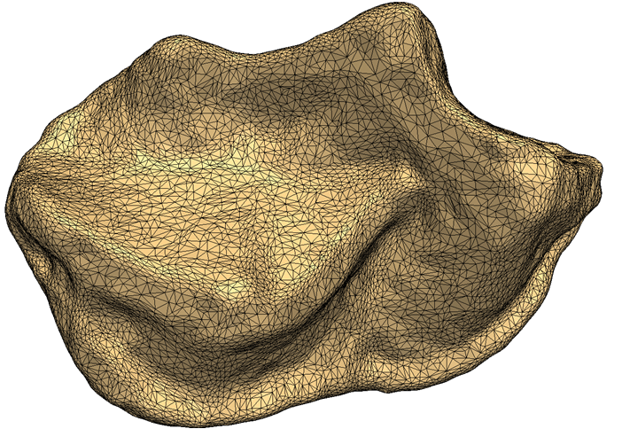
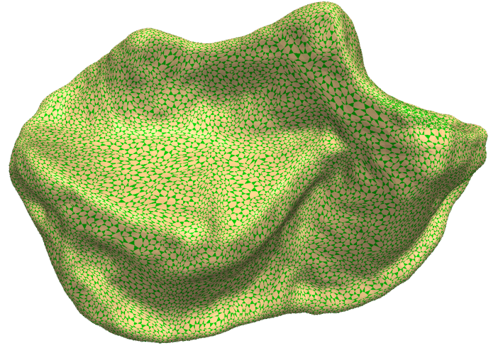
Discrete mesh	Mid-edge mesh
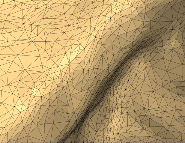
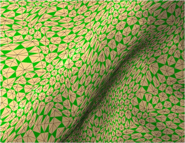
Surface mesh zoom-in	Mid-edge mesh zoom-in

Figure 11. A mammalian tooth surface mesh, with the corresponding mid-edge mesh. In the mid-edge mesh, the faces are the smaller green triangles within the faces of the surface mesh.

This flattening procedure maps the boundary of the mesh onto a region with a straight horizontal slit (see Figure 12, where the boundary points are marked in red) [20]. We can assume, without loss of generality, that this slit coincides with the interval $[-2,2]\subset\mathbb{C}$. Now applying the inverse of the holomorphic map $z=w+\frac{1}{w}$ maps $\mathbb{C}\setminus[-2,2]$ conformally to the disk $\mathcal{D}$, with the slit at $[-2,2]$ mapped to the boundary of the disk. It follows that when this map is applied to our flattened mid-edge mesh, its image is a mid-edge mesh in the unit disk, with the boundary of the disk corresponding to the boundary of our (disk-like) surface. (See Figure 12.) We shall denote by $\Phi:\textbf{{V}}\rightarrow\mathbb{C}$ the composition of these different conformal and discrete-conformal maps, from the original mid-edge mesh to the corresponding mid-edge mesh in the unit disk.

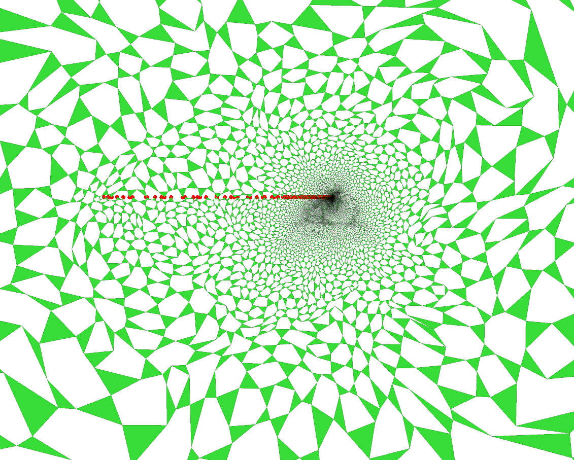
Mid-edge uniformization	Uniformization Zoom-in
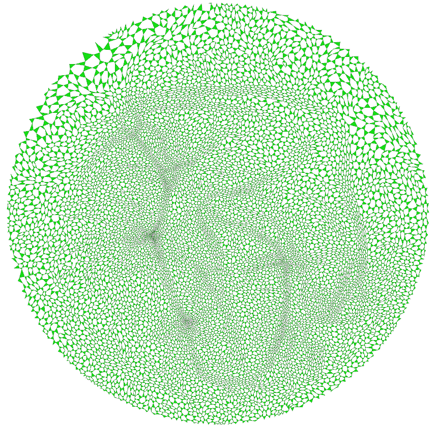
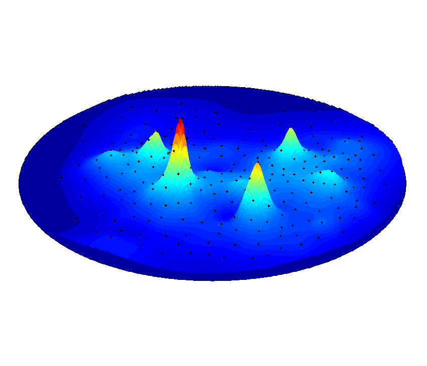
After mapping to the disk	Interpolated conformal factor

Figure 12. The discrete conformal transform to the unit disk for the surface of Figure 11, and the interpolation of the corresponding discrete conformal factors (plotted with the JET color map in Matlab). The red points in the top row’s images show the boundary points of the surface.

Next, we define the Euclidean discrete conformal factors, defined as the density, w.r.t. the Euclidean metric, of the mid-edge triangles (faces), i.e.

$$\mu^{E}_{\textbf{{f}}_{r,s,t}}=\frac{\mbox{\rm{vol}}_{\mathds{R}^{3}}(\textbf{{f}}_{r,s,t})}{\mbox{\rm{vol}}(\Phi(\textbf{{f}}_{r,s,t}))}.$$

Note that according to this definition, we have

$$\int_{\Phi(\textbf{{f}}_{r,s,t})}\,\mu^{E}_{\textbf{{f}}_{r,s,t}}\,d\mbox{\rm{\footnotesize{vol}}}_{E}\,=\,\frac{\mbox{\rm{vol}}_{\mathds{R}^{3}}(\textbf{{f}}_{r,s,t})}{\mbox{\rm{vol}}_{E}\left(\Phi(\textbf{{f}}_{r,s,t})\right)}\,\mbox{\rm{vol}}_{E}\left(\Phi(\textbf{{f}}_{r,s,t})\right)\,=\,\mbox{\rm{vol}}_{\mathds{R}^{3}}(\textbf{{f}}_{r,s,t}),$$

where $\mbox{\rm{vol}}_{E}$ denotes the standard Lebesgue (Euclidean) volume element in $\mathcal{D}$, and $\mbox{\rm{\footnotesize{vol}}}_{\mathbb{R}^{3}}(\textbf{{f}})$ stands for the area of f as induced by the standard Euclidean volume element in $\mathbb{R}^{3}$. The discrete Euclidean conformal factor at a mid-edge vertex $\textbf{{v}}_{r}$ is then defined as the average of the conformal factors for the two faces $\textbf{{f}}_{r,s,t}$ and $\textbf{{f}}_{r,s^{\prime},t^{\prime}}$ that touch in $\textbf{{v}}_{r}$, i.e.

$$\mu^{E}_{\textbf{{v}}_{r}}\,=\,\frac{1}{2}\,\left(\mu^{E}_{\textbf{{f}}_{r,s,t}}\,+\,\mu^{E}_{\textbf{{f}}_{r,s^{\prime},t^{\prime}}}\right).$$

Figure 12 illustrates the values of the Euclidean conformal factor for the mammalian tooth surface of earlier figures. The discrete hyperbolic conformal factors are defined according to the following equation, consistent with the convention adopted in section 1,

(B.1) $$\mu^{H}_{\textbf{{v}}_{r}}\,=\,\mu^{E}_{\textbf{{v}}_{r}}\,\left(1-|\Phi(\textbf{{v}}_{r})|^{2}\right)^{2}.$$

As before, we shall often drop the superscript $H$: unless otherwise stated, $\mu=\mu^{H}$, and $\nu=\nu^{H}$.

The (approximately) conformal mapping of the original mesh to the disk is completed by constructing a smooth interpolant $\Gamma_{\mu}:\mathcal{D}\rightarrow\mathbb{R}$, that interpolates the discrete conformal factor so far defined only at the vertices in $\Phi(\textbf{{V}})$; $\Gamma_{\nu}$ is constructed in the same way. In practice we use Thin-Plate Splines, i.e. functions of the type

(B.2) $$\Gamma_{\mu}(z)=p_{1}(z)\,+\,\sum_{i}\,b_{i}\,\psi(|z-z_{i}|)\,,$$

where $\psi(r)=r^{2}\log(r^{2})$, $p_{1}(z)$ is a linear polynomial in $x^{1},x^{2}$, and $b_{i}\in\mathbb{C}$; $p_{1}$ and the $b_{i}$ are determined by the data that need to be interpolated. Similarly $\Gamma_{\nu}(w)\,=\,q_{1}(w)\,+\,\sum_{j}\,c_{j}\,\psi(|w-w_{j}|)$ for some constants $c_{j}\in\mathbb{C}$ and a linear polynomial $q_{1}(w)$ in $y^{1},y^{2}$. We use as interpolation centers two point sets $Z=\left\{z_{i}\right\}_{i=1}^{n},$ and $W=\left\{w_{j}\right\}_{j=1}^{p}$ that are uniformly distributed over the surfaces $\mathcal{M}$ and $\mathcal{N}$ (resp.), they are (relatively small) subsets of the mid-edge mesh vertex sets. In practice we calculate these (sub) sample sets by starting from an initial random seed on the surface (which will itself not be included in the set), and take the geodesic furthest point in V (we approximate geodesic distances with Dijkstra’s algorithm) from the seed as the initial point of the sample set. One then keeps repeating this procedure, selecting at each iteration the point that lies at the furthest geodesic distance from the set of points already selected. This algorithm is known as the Farthest Point Algorithm (FPS) [8]. An example of the output of this algorithm, using geodesic distances on a disk-type surface, is shown in Figure 13. Further discussion of practical aspects of Voronoi sampling of a surface can be found in [4].

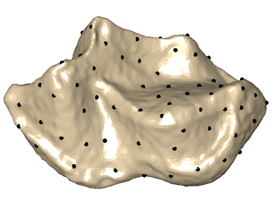
Figure 13. Sampling of the surface of Figure 11 obtained by the Farthest Point Algorithm.

Once the sample sets $Z$ and $W$ are determined we project them to the uniformization space using $\Phi$. The bottom-right part of Figure 12 shows the result of the interpolation based on the centers $Z,W$ (shown as black points).

To compute the explicit Thin-Plane-Splines (B.2), we use a standard smoothing Thin-Plate Spline procedure:

$$\Gamma_{\mu}(z)=\mathop{\mathrm{argmin}}_{\gamma}\left\{\lambda\sum_{r}\left|\mu_{\textbf{{v}}_{r}}-\gamma(\Phi(\textbf{{v}}_{r}))\right|^{2}+(1-\lambda)\int_{\mathcal{D}}\left(\frac{\partial^{2}\gamma}{(\partial x^{1})^{2}}\right)^{2}+\left(\frac{\partial^{2}\gamma}{\partial x^{1}\partial x^{2}}\right)^{2}+\left(\frac{\partial^{2}\gamma}{(\partial x^{2})^{2}}\right)^{2}dx^{1}\wedge dx^{2}\right\},$$

where the minimization is over all $\gamma$ in the appropriate Sobolev space and where we picked the values $0.95-0.99$ manually (it was fixed per dataset of surfaces) for the smoothing factor $\lambda$ to avoid over-fitting the data. We noticed that $\lambda$ does not have large effect on the results.

In our implementation we assumed we have a smooth representation of the conformal factors $\mu(z)=\Gamma_{\mu}(z)$, $\nu(w)=\Gamma_{\nu}(w)$ and we simply use the notation $\mu,\nu$ for these approximations.

To conclude this whirlwind description of the algorithm and ideas we use for discrete uniformization, we provide a short exposition on discrete and conjugate discrete harmonic functions on triangular meshes as in [7, 24, 25, 26], and show how we use them to conformally flatten disk-type ( or even just simply connected) triangular meshes.

Discrete harmonic functions are defined using a variational principle in the space of continuous piecewise linear functions defined over the mesh $PL_{\mathcal{M}}$ ([7]), as follows. Let us denote by $\phi_{i}(z),$ $i=1,..,m,$ the scalar functions that satisfy $\phi_{j}(v_{i})=\delta_{i,j}$ and are affine on each triangle $f_{i,j,k}\in F$. Then, the (linear) space of continuous piecewise-linear function on $M$ can be written in this basis:

$$PL_{M}=\left\{\sum_{i=1}^{m}u_{i}\phi_{i}(z)\ \mid\ (u_{1},...,u_{m})^{T}\in\mathbb{R}^{m}\right\}.$$

Next, the following quadratic form is defined over $PL_{M}$:

(B.3) $$E_{Dir}(u)=\sum_{f\in F}\int_{f}\left\langle\nabla u,\nabla u\right\rangle d\mbox{\rm{\footnotesize{vol}}}_{\mathbb{R}^{3}},$$

where $\left\langle\cdot\right\rangle=\left\langle\cdot\right\rangle_{\mathbb{R}^{3}}$ denotes the inner-product induced by the ambient Euclidean space, and $d\mbox{\rm{\footnotesize{vol}}}_{\mathbb{R}^{3}}$ is the induced volume element on $f$. This quadratic functional, the Dirichlet energy, can be written as follows:

(B.4) $$E_{Dir}\left(\sum_{i}u_{i}\phi_{i}\right)=\sum_{i,j=1}^{m}u_{i}u_{j}\left[\sum_{f\in F}\int_{f}\left\langle\nabla\phi_{i},\nabla\phi_{j}\right\rangle\right]d\mbox{\rm{\footnotesize{vol}}}_{\mathbb{R}^{3}}=\sum_{i,j=1}^{m}u_{i}u_{j}\int_{M}\left\langle\nabla\phi_{i},\nabla\phi_{j}\right\rangle d\mbox{\rm{\footnotesize{vol}}}_{\mathbb{R}^{3}}.$$

The discrete harmonic functions are then defined as the functions $u\in PL_{M}$ that are critical for $E_{Dir}(u)$, subject to some constraints on the boundary of $M$. The linear equations for discrete harmonic function $u\in PL_{M}$ are derived by partial derivatives of $E_{Dir}$, (B.4) w.r.t. $u_{i},i=1,..,m$:

(B.5) $$\frac{\partial E_{Dir}(u)}{\partial u_{k}}=2\sum_{i=1}^{m}u_{i}\left[\sum_{f\in F}\int_{f}\left\langle\nabla\phi_{i},\nabla\phi_{k}\right\rangle\right]d\mbox{\rm{\footnotesize{vol}}}_{\mathbb{R}^{3}}=2\int_{M}\left\langle\nabla u,\nabla\phi_{k}\right\rangle d\mbox{\rm{\footnotesize{vol}}}_{\mathbb{R}^{3}}=2\int_{R_{k}}\left\langle\nabla u,\nabla\phi_{k}\right\rangle d\mbox{\rm{\footnotesize{vol}}}_{\mathbb{R}^{3}},$$

where $R_{k}\subset M$ is the 1-ring neighborhood of vertex $v_{k}$. The last equality uses that $\phi_{k}$ is supported on $R_{k}$.

Now, let $u=\sum_{i}u_{i}\phi_{i}$ be a discrete harmonic function. Pinkall and Polthier observed that conjugating the piecewise-constant gradient field $\nabla u$ (constant on each triangle $f\in F$), i.e. rotating the gradient $\nabla u$ in each triangle $f$ by $\pi/2$ in the positive ( = counterclockwise) sense (we assume $M$ is orientable), results in a new vector field $*du=Jdu$ with the special property that its integrals along (closed) paths that cross edges only at their mid-points are systematically zero (see for example [26]). This means in particular that we can define a piecewise linear function $*u$ such that its gradient satisfies $d*u=*du$ and that is furthermore continuous through the mid-edges $\textbf{{v}}\in\textbf{{V}}$. The space of piecewise-linear functions on meshes that are continuous through the mid-edges is well-known in the finite-element literature, where it is called $ncPL_{M}$, the space of non-conforming finite elements [3]. The Dirichlet form (B.3) is defined over the space of non-conforming elements $ncPL_{M}$ as well; the non-conforming discrete harmonic functions are defined to be the functions $v\in ncPL_{M}$ that are critical for $E_{Dir}$ and that satisfy some constraints on the mid-edges of the boundary of the mesh. Polthier [26] shows that if $u\in PL_{M}$ is a discrete harmonic function, then $*u\in ncPL_{M}$ is also discrete harmonic, with the same Dirichlet energy, and vice-versa. Solving for the discrete harmonic function after fixing values at the boundaries amounts to solving a sparse linear system which is explicitly given in [26].

This theory can be used to define discrete conformal mappings, and used to flatten a mesh in a “discrete conformal” manner, as follows. The flattening is done by constructing a pair of conjugate piecewise linear functions $(u,*u)$ where $u\in PL_{M}$, $*u\in ncPL_{M}$, and the flattening map $\Phi:\textbf{{M}}\rightarrow\mathbb{C}$ is given by

(B.6) $$\Phi=u+\textbf{\footnotesize{i}}*u.$$

Since $d*u=Jdu$, $\Phi$ is a similarity transformation on each triangle $f\in F$. Furthermore, $\Phi$ is continuous through the mid-edge points $\textbf{{v}}_{r}\in\textbf{{V}}$; $\Phi$ is thus well-defined on the points in V and maps them to the complex plane.

The function $u$ is defined by choosing an arbitrary triangle $f_{out}\in F$, excising it from the mesh, setting the values of $u$ at two of $f_{out}$’s vertices $u_{i_{1}},u_{i_{2}}$ to $0$ and $1$, respectively, and then solving for the discrete harmonic $u$ that satisfies these constraints. See for example Figure 12 (top-left); the “missing mid-edge face” corresponding to the excised face $f_{out}$ would have connected the three mid-edge vertices that have a only one mid-edge face touching them. The conjugate function $*u$ is constructed by a simple conjugation (and integration) process as described in [26] and [20].

A surprising property of the Discrete Uniformization $\Phi$ as it is defined above, which nicely imitates the continuous theory (see [31]) is that it takes the boundaries of $\mathcal{M}$ to horizontal slits, see Figure 12, top row (boundary vertices colored in red). This property allows us to easily construct a closed form analytic map (with “analytic” in its standard complex analytic sense) that will further bijectively map the entire complex plane $\mathbb{C}$ minus the slit to the open unit disk, completing our Uniformization procedure.

The proof of this property is similar to that for Proposition 35 in [26]; see also [20]. More precisely:

Theorem B.1.

Let $\Phi:\textbf{{M}}\rightarrow\mathbb{C}$ be the flattening map from the mid-edge mesh M of a mesh $\mathcal{M}$ with boundary, using a discrete harmonic and conjugate harmonic pair as described above. Then, for each connected component of the boundary of $\mathcal{M}$, the mid-edge vertices of boundary edges are all mapped onto one line segment parallel to the real axis.

Proof.

Suppose $u=\sum_{i}u_{i}\phi_{i}(\cdot)$ is a discrete harmonic, piecewise linear and continuous function, defined at each vertex $v_{i}\in V$, excluding the two vertices of the excised triangle for which values are prescribed; then we have, by (B.5),

(B.7) $$\int_{R_{i}}\langle\nabla\phi_{i},\nabla u\rangle d\mbox{\rm{\footnotesize{vol}}}_{\mathbb{R}^{3}}=0,$$

Next, consider a boundary vertex $v_{j}$ of the mesh $\mathcal{M}$. Denote by $\textbf{{v}}_{r},\textbf{{v}}_{s}$ the mid-edge vertices on the two boundary edges touching vertex $v_{j}$. We will show that $*u(\textbf{{v}}_{r})=*u(\textbf{{v}}_{s})$; this will imply the theorem, since $*u$ gives the imaginary coordinate for the images of the mid-edge vertices under the flattening map (see (B.6)) . Observe that on the triangle $f_{i,j,k}$,

(B.8) $$\nabla\phi_{j}=\frac{J(v_{i}-v_{k})}{2\,\mbox{\rm{\footnotesize{vol}}}_{\mathbb{R}^{3}}(f_{i,j,k})}.$$

Recalling that $\nabla*u=J\nabla u$, using (B.8), and $J^{T}=-J$, we obtain

$$*u(\textbf{{v}}_{r})-*u(\textbf{{v}}_{s}) =\int_{\gamma}d*u=\int_{\gamma}*du=\sum_{f_{i,j,k}\ni v_{j}}\left\langle J\nabla u\mid_{f_{i,j,k}},\frac{1}{2}(v_{i}-v_{k})\right\rangle$$

$$=\sum_{f_{i,j,k}\ni v_{j}}\left\langle\nabla u\mid_{f_{i,j,k}},\frac{1}{2}J^{T}(v_{i}-v_{k})\right\rangle=\sum_{f_{i,j,k}\ni v_{j}}\left\langle\nabla u\mid_{f_{i,j,k}},-\nabla\phi_{j}\mid_{f}\right\rangle\mbox{\rm{\footnotesize{vol}}}_{\mathbb{R}^{3}}(f)$$

$$=-\int_{M}\left\langle\nabla u,\nabla\phi_{j}\right\rangle d\mbox{\rm{\footnotesize{vol}}}_{\mathbb{R}^{3}}=0,$$

where $\gamma$ is the piecewise linear path starting at $\textbf{{v}}_{r}$ and passing through the mid-edge vertices of the 1-ring neighborhood of $v_{j}$ ending at $\textbf{{v}}_{s}$. The last equality is due to (B.5). ∎

A natural question, when dealing with any type of finite-element approximation, concerns convergence as the mesh is refined: convergence in what sense, and at what rate? For discrete harmonic functions over meshes, this convergence is discussed in [15, 25]. These convergence results are in the weak sense; this motivated our defining the discrete conformal factors $\mu_{\textbf{{f}}}$ via integrated quantities (volumes) in Section 2.

Finally, we note that the method presented here for Discrete Uniformization is just one option among several; other authors have suggested other techniques; for example [12]. Typically, this part of the complete algorithm described in this paper could be viewed as a “black box”: the remainder of the algorithm would not change if one method of Discrete Uniformization is replaced by another.

Appendix C

In this Appendix we prove a lemma used in the proof of Theorem 2.6.

Lemma The $N\times N$ matrices $\pi$ satisfying

(C.1) $$\left\{\begin{array}[]{c}\sum_{i}\pi_{ij}\leq 1\\ \sum_{j}\pi_{ij}\leq 1\\ \pi_{ij}\geq 0\\ \sum_{i,j}\pi_{ij}=M<N\end{array}\right.$$

constitute a convex polytope $\mathcal{P}$ of which the extremal points are exactly those $\pi$ that satisfy all these constraints, and that have all entries equal to either 0 or 1.

Remark. Note that the matrices $\pi\in\mathcal{P}$ with all entries in $\{0,1\}$ have exactly $M$ entries equal to 1, and all other entries equal to zero; if one removes from these matrices all rows and columns that consist of only zeros, what remains is a $M\times M$ permutation matrix.

Proof.

$\mathcal{P}$ can be considered as a subset of $\mathbb{R}^{N^{2}}$, with all entries nonnegative, summing to $M$. The two inequalities in (C.1) imply that the entries of any $\pi\in\mathcal{P}$ are bounded by 1. These inequalities can also be rewritten as the constraint that every entry of $A\mathcal{P}-b\in\mathbb{R}^{2N}$ is non positive, where $A$ is a $\mathbb{R}^{2N}\times\mathbb{R}^{N^{2}}$ matrix, and $b$ is a vector in $\mathbb{R}^{2N}$. It follows that $\mathcal{P}$ is a (bounded) convex polytope in $\mathbb{R}^{N^{2}}$.

If $\pi\in\mathcal{P}\subset\mathbb{R}^{N^{2}}$ has entries equal to only 0 or 1, then $\pi$ must be an extremal point of $\mathcal{P}$ by the following argument. If $\pi_{\ell}=1$, and $\pi$ is a nontrivial convex combination of $\pi^{1}$ and $\pi^{2}$ in $\mathcal{P}$, then

$$\pi=\lambda\,\pi^{1}\,+\,(1-\lambda)\,\pi^{2}\,\mbox{ with }\lambda\in(0,1)\,\Longrightarrow 1=\lambda\,\pi^{1}_{\ell}\,+\,(1-\lambda)\,\pi^{2}_{\ell}\,\mbox{ with }\pi^{1}_{\ell}\,,\,\pi^{2}_{\ell}\geq 0\Longrightarrow\pi^{1}_{\ell}=\pi^{2}_{\ell}=1~{}.$$

A similar argument can be applied for the entries of $\pi$ that are 0. It follows that we must have $\pi^{1}=\pi=\pi^{2}$, proving that $\pi$ is extremal.

It remains thus to prove only that $\mathcal{P}$ has no other extremal points. To achieve this, it suffices to prove that the extremal points of $\mathcal{P}$ are all integer vectors, i.e. vectors all entries of which are integers – once this is established, the Lemma is proved, since the only integer vectors in $\mathcal{P}$ are those with all entries in $\{0,1\}$.

To prove that the extremal points of $\mathcal{P}$ are all integer vectors, we invoke the Hoffman-Kruskal theorem (see [17], Theorem 7C.1), which states that, given a $L\times K$ matrix $\mathbb{M}$, with all entries in $\{-1,0,1\}$, and a vector $b\in\mathbb{R}^{L}$ with integer entries, the vertices of the polytope defined by $\{x\in\mathbb{R}^{K}\,;\,(\mathbb{M}x)_{\ell}\leq b_{\ell}\,\mbox{ for }\,\ell=1,\ldots,L\}$ are all integer vectors in $\mathbb{R}^{K}$ if and only if the matrix $\mathbb{M}$ is totally unimodular, i.e. if and only if every square submatrix of $\mathbb{M}$ has determinant 1, 0 or $-1$.

We first note that (C.1) can indeed be written in this special form. The equality $\sum_{i,j}\pi_{ij}=M$ can be recast as the two inequalities $\sum_{i,j}\pi_{ij}\leq M$ and $-\,\sum_{i,j}\pi_{ij}\leq-M$. The full system (C.1) can then be written as $(\mathbb{M}\pi)_{\ell}\leq b_{\ell}$ for $\ell=1,\ldots,L$, where $\mathbb{M}$ is a $(2N+2+N^{2})\times N^{2}$ matrix constructed as follows. Its first $2N$ rows correspond to the constraints on the sums over rows and columns; the entries of the next row are all 1, and of the row after that, all $-1$ – these two rows correspond to the constraint $\sum_{i,j}\pi_{ij}=M$; the final $N^{2}\times N^{2}$ block is diagonal, with all its diagonal entries equal to $-1$. The first $2N$ entries of $b$ are 1; the next 2 entries are $M$ and $-M$; its final $N^{2}$ entries are 0. By the Hoffman-Kruskal theorem it suffices thus to show that $\mathbb{M}$ is totally unimodular.

Because the last $N^{2}$ rows, the bottom rows of $\mathbb{M}$, have only one non-zero entry, which equals $-1$, we can disregard them. Indeed, if we take a square submatrix of $\mathbb{M}$ that includes (part of) one of these bottom rows, then the determinant of the submatrix is 0 if only zero entries of the bottom row ended up in the submatrix; if the one -1 entry of the bottom row is an entry in the submatrix, then the determinant is, possibly up to a sign change, the same as if that row and the column of the $-1$ entry are removed. By this argument, we can remove all the rows of the submatrix partaking of the bottom rows of $\mathbb{M}$.

We thus have to check unimodularity only for $\mathbb{M}^{\prime}$, the submatrix of $\mathbb{M}$ given by its first $2N+2$ rows. If any submatrix contains (parts of) both the $(2N+1)$st and the $(2N+2)$nd row, then the determinant is automatically zero, since the second of these two rows equals the first one, multiplied by -1. This reduces the problem to checking that $\mathbb{M}^{\prime\prime}$, the submatrix of $\mathbb{M}$ given by its first $2N+1$ rows, is totally unimodular.

We now examine the top $2N$ rows of $\mathbb{M}^{\prime\prime}$ more closely. A little scrutiny reveals that it is, in fact, the adjacency matrix $\mathbb{G}$ of the complete bipartite graph with $N$ vertices in each part. It is well-known (see e.g. Theorem 8.3 in [29]) that this adjacency matrix is totally unimodular, so any square submatrix of $\mathbb{M}^{\prime\prime}$ that does not involve the $(2N+1)$st row of $\mathbb{M}^{\prime\prime}$ is already known to have determinant 0, 1 or $-1$. We thus have to check only submatrices that involve the last row, i.e. matrices that consist of a $(n-1)\times n$ submatrix of $\mathbb{G}$, with an added $n$th row with all entries equal to 1. We’ll denote such submatrices by $\mathbb{G}^{\prime}$.

We can then use a simple induction argument on $n$ to finish the proof. The case $n=2$ is trivial. In proving the induction step for $n=m$, we can assume that each of the top $m-1$ rows of our $m\times m$ submatrix $\mathbb{G}^{\prime}$ contains at least two entries equal to 1, since otherwise the determinant of $\mathbb{G}^{\prime}$ would automatically be 0, 1 or -1 by induction.

The first $m-1$ rows of $\mathbb{G}^{\prime}$ correspond to vertices in the bipartite graph, and can thus be partitioned into two sets $S_{1}$ and $S_{2}$, based on which of the two parts of $N$ vertices in the graph they pertain to. Let us call $S$ the larger of $S_{1}$ and $S_{2}$; $S$ consists of at least $\lceil\frac{m-1}{2}\rceil$ rows. Let us examine the $(\#S)\times m$ sub-matrix $\mathbb{G}^{\prime\prime}$ constructed from exactly these rows. We know that each column of $\mathbb{G}^{\prime\prime}$ has exactly one entry $1$, since all the rows of $\mathbb{G}^{\prime\prime}$ correspond to the same group of vertices in the bipartite graph. Therefore, summing all the rows of $\mathbb{G}^{\prime\prime}$ gives a vector $v$ of only zeros and ones; since each row in $\mathbb{G}^{\prime\prime}$ contains at least two entries equal to 1, the sum of all entries in $v$ is at least $2\left(\lceil\frac{m-1}{2}\rceil\right)\geq m-1$. The vector $v$ has thus at least $m-1$ entries equal to $1$; the remaining $m$th entry of this linear combination of the top $m-1$ rows of $\mathbb{G}^{\prime}$ is either 1 or 0. In the first case, the determinant of $\mathbb{G}^{\prime}$ vanishes, since its last row also consists of only ones. In the second case, we can subtract $v$ from the last row of $\mathbb{G}^{\prime}$ without changing the value of the determinant; the resulting last row has all entries but one equal to 0, with a remaining entry equal to 1. The determinant is then given by the minor of this remaining entry, and is thus 0, 1 or -1 by the unimodularity of $\mathbb{G}$. ∎

Appendix D

In this Appendix we provide a constructive procedure and convergence analysis for approximating the optimal transport cost between general separable complete compact metric spaces $(\mathcal{X},d_{\mathcal{X}}),(\mathcal{Y},d_{\mathcal{Y}})$ each equipped with a probability measure $\mu\in P(\mathcal{X}),\nu\in P(\mathcal{Y})$, where $P(\mathcal{X})$ ($P(\mathcal{Y})$) denotes the set of probability measures on $\mathcal{X}$ ($\mathcal{Y}$). In the context of the algorithm previously described $\mathcal{X},\mathcal{Y}$ are the two given surfaces, $d_{\mathcal{X}},d_{\mathcal{Y}}$ the corresponding geodesic distance metric functions, and $\mu,\nu$ the area measures of the surfaces induced from the metric tensors, respectively. Since $R,\mu,\nu$ are kept fixed through this discussion, we will denote, for brevity, $c(x,y)=d^{R}_{\mu,\nu}(x,y)$.

The Kantorovich optimal transportation cost of the measures $\mu,\nu$ is defined as

(D.1) $$T_{c}(\mu,\nu)=\mathop{\inf}_{\pi\in\Pi(\mu,\nu)}\int_{X\times Y}c(x,y)d\pi(x,y),$$

where $\Pi(\mu,\nu)\subset P(\mathcal{X}\times\mathcal{Y})$ is the set of probability measures on $\mathcal{X}\times\mathcal{Y}$ with marginals $\mu,\nu$, that is, $\pi\in\Pi(\mu,\nu)\Rightarrow\pi(A\times\mathcal{Y})=\mu(A)$ and $\pi(\mathcal{X}\times A^{\prime})=\nu(A^{\prime})$, for all Borel $A\subset\mathcal{X},A^{\prime}\subset\mathcal{Y}$.

The main goal of this section is to present an approximation result for $T_{c}(\mu,\nu)$ in this general framework. In particular, this result will assure the convergence of our algorithm.

To our knowledge, the only related result talks merely about convergence of the optimal cost (e.g., [32], Theorem 5.20). However, for practical applications it is important to control the rate of convergence, and therefore to be able to compute error-bounded approximations.

In the specific case of $c(x,y)=\left\|x-y\right\|^{2}$ there are good approximation techniques that rely on the polar decomposition of Brenier, for example the work of Haker and collaborators [13]. However, as far as we are aware no approximation result is known in the general metric case as required here.

We will show that solving discrete mass-transportation between two sets of discrete measures $\mu_{S},\nu_{T}$, based on Voronoi diagrams of two collections of points $S=\left\{s_{i}\right\}\subset\mathcal{X},T=\left\{t_{j}\right\}\subset\mathcal{Y}$, achieve linear approximation order to the continuous limit mass-transport cost $T_{c}(\mu,\nu)$:

$$\Big{|}T_{c}(\mu,\nu)-T_{c}(\mu_{S},\nu_{T})\Big{|}\leq\omega_{c}\left(2h\right),$$

where $\omega_{c}(\alpha)$ is the modulus of continuity of $c$ defined by

$$\omega_{c}(\alpha)=\sup_{d_{\mathcal{X}}(x,x^{\prime})+d_{\mathcal{Y}}(y,y^{\prime})<\alpha}\left|c(x,y)-c(x^{\prime},y^{\prime})\right|,$$

and $h=\max\{\eta(S),\eta(T)\}$, where the fill distances $\varphi_{\mathcal{X}}(S),\varphi_{\mathcal{Y}}(T)$ are defined as before by

(D.2) $$\varphi_{\mathcal{X}}(S)=\sup\Big{\{}r\in\mathbb{R}\ \Big{|}\ \exists x\in\mathcal{X}\ s.t.\ B_{\mathcal{X}}(x,r)\cap S=\emptyset\Big{\}},$$

where $B_{\mathcal{X}}(x,r)=\{q\in\mathcal{X}\ |\ d_{\mathcal{X}}(x,q)<r\}$ (and similarly for $\varphi_{\mathcal{Y}}(T)$).

In particular, for Lipschitz cost function $c$ with Lipschitz constant $\lambda$, we have the following bound for the error in the approximation:

(D.3) $$\Big{|}T_{c}(\mu,\nu)-T_{c}(\mu_{S},\nu_{T})\Big{|}\leq 2\lambda h.$$

In turn, this result suggests an algorithm for approximating $T_{c}(\mu,\nu)$: simply spread points $S\subset\mathcal{X}$ and $T\subset\mathcal{Y}$ such that no big empty space is left uncovered, then compute $T_{c}(\mu_{S},\nu_{T})$ using linear-programming solver.

D.1. Voronoi cells and discrete measures

Let $(\mathcal{X},d_{\mathcal{X}},\mu),(\mathcal{Y},d_{\mathcal{Y}},\nu)$ be two compact, complete, separable metric spaces with probability measures defined over the Borel sets.

The discrete measures will based on discrete sets of points $S=\{s_{i}\}_{i=1}^{m}\subset\mathcal{X}$,$T=\{t_{i}\}_{i=1}^{n}\subset\mathcal{Y}$ and the coarseness of the sets will be measured by means of the so-called fill-distance $\varphi_{\mathcal{X}}(S),\varphi_{\mathcal{Y}}(T)$ of the sets $S,T$. The fill-distance of $S\subset\mathcal{X}$ is defined in eq. (D.2). The sets get “finer” as $\max\left\{\varphi_{\mathcal{X}}(S),\varphi_{\mathcal{Y}}(T)\right\}\rightarrow 0$.

Definition D.1.

For set of points $S=\{s_{i}\}_{i=1}^{m}\subset\mathcal{X}$ we define

(D.4) $$O^{S}_{i}=\Big{\{}x\in\mathcal{X}\ \Big{|}\ d_{\mathcal{X}}(x,s_{i})<\min_{j\neq i}d_{\mathcal{X}}(x,s_{j})\Big{\}}.$$

(D.5) $$C^{S}_{i}=\Big{\{}x\in\mathcal{X}\ \Big{|}\ d_{\mathcal{X}}(x,s_{i})\leq\min_{j\neq i}d_{\mathcal{X}}(x,s_{j})\Big{\}}.$$

Then, Voronoi cells for the point set $S$ is any collection of sets $\{V_{i}\}_{i=1}^{m}$ satisfying

1. $\cup_{i=1}^{m}V_{i}=\mathcal{X}$.

2. $V_{i}\cap V_{j}=\emptyset$ for $i\neq j$.

3. $O^{S}_{i}\subset V_{i}\subset C^{S}_{i}$, for all $i=1,..,m$.

We will prove now a simple lemma, for later use, connecting the fill-distance with the geometry of the Voronoi cells.

Lemma D.2.

Let $S=\{s_{i}\}_{i=1}^{m}\subset\mathcal{X}$. If $\{V_{i}\}_{i=1}^{m}$ is a collection of Voronoi cells corresponding to $S$, then for all $\varepsilon>0$,

$$V_{i}\subset B(s_{i},\varphi_{\mathcal{X}}(S)+\varepsilon),\ \ i=1,..,m$$

Proof.

Take $x\notin B(s_{i},\varphi_{\mathcal{Y}}(S)+\varepsilon)$.

By the definition of the fill-distance we have that

$$B\left(x,\varphi_{\mathcal{X}}(S)+\frac{\varepsilon}{2}\right)\cap S\neq\emptyset.$$

That is, there exists $s_{k}\in S$, $k\neq i$, such that

$$d_{\mathcal{X}}(x,s_{k})<\varphi_{\mathcal{X}}(S)+\frac{\varepsilon}{2}.$$

However,

$$d_{\mathcal{X}}(x,s_{i})\geq\varphi_{\mathcal{X}}(S)+\varepsilon>d_{\mathcal{X}}(x,s_{k}).$$

Hence from the definition of the Voronoi cells

$$x\in\mathcal{X}\setminus C^{S}_{i}\subset\mathcal{X}\setminus V_{i},$$

that is $x\notin V_{i}$. ∎

Given a set of points and a Voronoi cell collection $S,\{V_{i}\}_{i=1}^{m}$ we define a discrete measure $\mu_{S}$ by

(D.6) $$\mu_{S}=\sum_{i=1}^{m}\mu(V_{i})\delta_{s_{i}},$$

where $\delta_{s_{i}}$ is the dirac measure centered at $s_{i}$. That is

$$\int_{\mathcal{X}}f\ d\mu_{S}=\sum_{i=1}^{m}\mu(V_{i})f(s_{i}).$$

Similarly we define Voronoi cell collection $\{W_{j}\}_{j=1}^{n}$ for point set $T\subset\mathcal{Y}$, and corresponding discrete measure $\nu_{T}$.

Let us prove that the discrete measures $\mu_{S},\nu_{T}$ converge in the weak sense to $\mu,\nu$. By weak convergence $\mu_{S}\rightarrow\mu$ of measure we mean (see for example [23]) that for every continuous bounded function $f:\mathcal{X}\rightarrow\mathbb{R}$ there exists

$$\int_{\mathcal{X}}f\ d\mu_{S}\longrightarrow\int_{\mathcal{X}}f\ d\mu\ ,\ \ \mathrm{as}\ \varphi_{\mathcal{X}}(S)\rightarrow 0.$$

Theorem D.3.

$\lim_{\varphi_{\mathcal{X}}(S)\rightarrow 0}\int_{\mathcal{X}}f\ d\mu_{S}=\int_{\mathcal{X}}f\ d\mu$, for all $f:\mathcal{X}\rightarrow\mathbb{R}$ bounded and continuous.

Proof.

$X$ is compact therefore $f$ is uniformly continuous. Take arbitrary $\varepsilon>0$, let $\delta(\varepsilon)>0$ be such that

$$x,x^{\prime}\in\mathcal{X}\ ,\ d_{\mathcal{X}}(x,x^{\prime})<\delta(\varepsilon)\ \Rightarrow\ \left|f(x)-f(x^{\prime})\right|<\varepsilon.$$

For $S$ with $\varphi_{\mathcal{X}}(S)<\delta(\varepsilon)$ we have

$$\left|\int_{\mathcal{X}}f\ d\mu-\int_{\mathcal{X}}f\ d\mu_{S}\right|=\left|\sum_{i=1}^{m}\int_{V_{i}}\left(f(x)-f(s_{i})\right)\ d\mu\right|\leq$$

$$\leq\sum_{i=1}^{m}\int_{V_{i}}\left|f(x)-f(s_{i})\right|\ d\mu\leq\sum_{i=1}^{m}\varepsilon\mu(V_{i})=\varepsilon,$$

where in the second to last transition we used the fact that $V_{i}\subset B(s_{i},\delta(\varepsilon))$ which we know is the case from Lemma D.2. ∎

Lastly, we will denote by $\Pi(\mu_{S},\nu_{T})\subset P(S\times T)$ the subset of probability measures on the discrete product space $S\times T$ with marginals $\mu_{S},\nu_{T}$.

D.2. Approximation of optimal cost

In this subsection we prove the main result of this appendix. Namely, that the optimal transport cost $T_{c}(\mu_{S},\nu_{T})$ of the discrete measures $\mu_{S},\nu_{T}$ is an $\varepsilon-$approximation to the optimal transport cost $T_{c}(\mu,\nu)$ of $\mu,\nu$ if the fill-distance $h=\max\{\varphi_{\mathcal{X}}(S),\varphi_{\mathcal{Y}}(T)\}<\frac{1}{2}\delta(\varepsilon)$, where $\delta(\varepsilon)$ is the uniform continuity constant of $c$.

Actually, we will prove a slightly stronger result: denote the sets

(D.7) $$\mathcal{A}=\Big{\{}\int_{\mathcal{X}\times\mathcal{Y}}c\ d\pi\ \Big{|}\ \pi\in\Pi(\mu,\nu)\Big{\}}\ \ ,\ \ \mathcal{B}=\Big{\{}\int_{\mathcal{X}\times\mathcal{Y}}c\ d\pi\ \Big{|}\ \pi\in\Pi(\mu_{S},\nu_{T})\Big{\}}.$$

We will show that the Hausdorff distance $d_{H}(\mathcal{A},\mathcal{B})\rightarrow 0$ as $h\rightarrow 0$. Where by Hausdorff distance of two sets $\mathcal{A},\mathcal{B}\subset\mathds{R}$ we mean

$$d_{H}(\mathcal{A},\mathcal{B})=\inf\Big{\{}r\Big{|}\ \mathcal{B}\subset U(\mathcal{A},r)\ ,\ \mathcal{A}\subset U(\mathcal{B},r)\Big{\}},$$

where $U(\mathcal{A},r)=\cup_{a\in\mathcal{A}}B(a,r)$ and $B(a,r)$ is the open ball of radius $r$ centered at $a$. Moreover, we will provide a linear (in $h$) bound controlling the convergence rate, for Lipschitz cost function $c$.

Theorem D.4.

If $c:\mathcal{X}\times\mathcal{Y}\longrightarrow\mathbb{R}_{+}$ is a continuous function, $\mathcal{X},\mathcal{Y}$ compact complete separable metric spaces. Let $h=\max\left\{\varphi_{\mathcal{X}}(S),\varphi_{\mathcal{Y}}(T)\right\}$ then,

$$d_{H}(\mathcal{A},\mathcal{B})\leq\omega_{c}(2h),$$

where $\mathcal{A},\mathcal{B}$ are defined in (D.7). In particular,

$$\Big{|}T_{c}(\mu,\nu)-T_{c}(\mu_{S},\nu_{T})\Big{|}\leq\omega_{c}(2h).$$

Proof.

Take arbitrary $S=\{s_{i}\}_{i=1}^{m}\subset\mathcal{X}$, $T=\{t_{i}\}_{j=1}^{n}\subset\mathcal{Y}$. Choose collections of Voronoi cells $\{V_{i}\}_{i=1}^{m}$, $\{W_{j}\}_{j=1}^{n}$ for $S,T$ respectively.

Now take $\pi\in\Pi(\mu,\nu)$.

Set

$$\Lambda=\sum_{i=1}^{m}\sum_{j=1}^{n}\pi(V_{i}\times W_{j})\delta_{s_{i},t_{j}}.$$

Then,

$$\Lambda(A\times\mathcal{Y})=\sum_{i=1}^{m}\sum_{j=1}^{n}\pi(V_{i}\times W_{j})\delta_{s_{i}}(A)=$$

$$\sum_{i=1}^{m}\pi(V_{i}\times\mathcal{Y})\delta_{s_{i}}(A)=\sum_{i=1}^{m}\mu(V_{i})\delta_{s_{i}}(A)=\mu_{S}(A).$$

Similarly

$$\Lambda(\mathcal{X}\times A^{\prime})=\nu_{T}(A^{\prime}).$$

Therefore

$$\Lambda\in\Pi(\mu_{S},\nu_{T}).$$

Moreover,

$$\Big{|}\int_{\mathcal{X}\times\mathcal{Y}}c\ d\pi-\int_{\mathcal{X}\times\mathcal{Y}}c\ d\Lambda\Big{|}=\Big{|}\sum_{i=1}^{m}\sum_{j=1}^{n}\int_{V_{i}\times W_{j}}\big{[}c(x,y)-c(s_{i},t_{j})\big{]}\ d\pi\Big{|}\leq$$

$$\sum_{i=1}^{m}\sum_{j=1}^{n}\int_{V_{i}\times W_{j}}\big{|}c(x,y)-c(s_{i},t_{j})\big{|}\ d\pi.$$

For $(x,y)\in V_{i}\times W_{j}$, we have $d_{\mathcal{X}}(x,s_{i})\leq\varphi_{\mathcal{X}}(S)$, $d_{\mathcal{Y}}(y,t_{j})\leq\varphi_{\mathcal{Y}}(T)$ which implies

(D.8) $$\left|c(x,y)-c(s_{i},t_{j})\right|\leq\omega_{c}\left(\varphi_{\mathcal{X}}(S)+\varphi_{\mathcal{Y}}(T)\right)\leq\omega_{c}(2h).$$

So we have

$$\left|\int_{\mathcal{X}\times\mathcal{Y}}c\ d\pi-\int_{\mathcal{X}\times\mathcal{Y}}c\ d\Lambda\right|\leq\omega_{c}(2h)\sum_{i=1}^{n}\sum_{j=1}^{n}\pi(V_{i}\times W_{j})=\omega_{c}(2h),$$

since $\left\{V_{i}\times W_{j}\right\}_{i,j=1,1}^{n,m}$ form a partition of $X\times Y$. So we proved that

$$\mathcal{A}\subset\overline{U(\mathcal{B},\omega_{c}(2h))}.$$

We now prove the other direction. Take $\Lambda\in\Pi(\mu_{S},\nu_{T})$.

Denote by $\mu\times\nu\big{|}_{V_{i}\times W_{j}}$ the product measure $\mu\times\nu$ restricted to $V_{i}\times W_{j}\subset\mathcal{X}\times\mathcal{Y}$.

That is,

$$\mu\times\nu\big{|}_{V_{i}\times W_{j}}(A\times A^{\prime})=\mu\times\nu\left((V_{i}\times W_{j})\cap(A\times A^{\prime})\right)=\mu(V_{i}\cap A)\nu(W_{j}\cap A^{\prime}).$$

Now pick

$$\pi=\sum_{i=1}^{m}\sum_{j=1}^{n}\frac{\Lambda(V_{i}\times W_{j})}{\mu(V_{i})\nu(W_{j})}\mu\times\nu\big{|}_{V_{i}\times W_{j}}.$$

Then,

$$\pi(A\times\mathcal{Y})=\sum_{i=1}^{m}\sum_{j=1}^{n}\frac{\Lambda(V_{i}\times W_{j})}{\mu(V_{i})\nu(W_{j})}\mu(V_{i}\cap A)\nu(W_{j}\cap\mathcal{Y})=$$

$$\sum_{i=1}^{m}\sum_{j=1}^{n}\frac{\Lambda(V_{i}\times W_{j})}{\mu(V_{i})}\mu\left(V_{i}\cap A\right)=$$

$$\sum_{i=1}^{m}\frac{\mu(V_{i}\cap A)}{\mu(V_{i})}\left[\sum_{j=1}^{n}\Lambda\left(V_{i}\times W_{j}\right)\right]=$$

$$\sum_{i=1}^{m}\frac{\mu(V_{i}\cap A)}{\mu(V_{i})}\Lambda\left(V_{i}\times\mathcal{Y}\right)=$$

$$\sum_{i=1}^{m}\frac{\mu(V_{i}\cap A)}{\mu(V_{i})}\mu(V_{i})=$$

$$\sum_{i=1}^{m}\mu(V_{i}\cap A)=\mu(\mathcal{X}\cap A)=\mu(A).$$

Similarly

$$\pi(\mathcal{X}\times A^{\prime})=\nu(A^{\prime}).$$

Therefore,

$$\pi\in\Pi(\mu,\nu).$$

Now,

$$\left|\int_{\mathcal{X}\times\mathcal{Y}}c\ d\pi-\int_{\mathcal{X}\times\mathcal{Y}}c\ d\Lambda\right|=$$

$$\left|\sum_{i=1}^{m}\sum_{j=1}^{n}\frac{\Lambda\left(V_{i}\times W_{j}\right)}{\mu(V_{i})\nu(W_{j})}\int_{V_{i}\times W_{j}}c\ d\left(\mu\times\nu\right)-\sum_{i=1}^{m}\sum_{j=1}^{n}c(s_{i},t_{j})\Lambda(V_{i}\times W_{j})\right|=$$

$$\left|\sum_{i=1}^{m}\sum_{j=1}^{n}\left[\frac{\Lambda\left(V_{i}\times W_{j}\right)}{\mu(V_{i})\nu(W_{j})}\int_{V_{i}\times W_{j}}c\ d\left(\mu\times\nu\right)-\frac{\Lambda\left(V_{i}\times W_{j}\right)}{\mu(V_{i})\nu(W_{j})}\int_{V_{i}\times W_{j}}c(s_{i},t_{j})\ d\left(\mu\times\nu\right)\right]\right|\leq$$

$$\sum_{i=1}^{m}\sum_{j=1}^{n}\frac{\Lambda\left(V_{i}\times W_{j}\right)}{\mu(V_{i})\nu(W_{j})}\int_{V_{i}\times W_{j}}\left|c(x,y)-c(s_{i},t_{j})\right|\ d\left(\mu\times\nu\right).$$

As before, for $(x,y)\in V_{i}\times W_{j}$, we have $d_{\mathcal{X}}(x,s_{i})\leq\varphi_{\mathcal{Y}}(S)$, $d_{\mathcal{Y}}(y,t_{j})\leq\varphi_{\mathcal{Y}}(T)$ therefore

$$\left|c(x,y)-c(s_{i},t_{j})\right|\leq\omega_{c}\left(\varphi_{\mathcal{X}}(S)+\varphi_{\mathcal{Y}}(T)\right)\leq\omega_{c}(2h).$$

And therefore

$$\left|\int_{\mathcal{X}\times\mathcal{Y}}c\ d\pi-\int_{\mathcal{X}\times\mathcal{Y}}c\ d\Lambda\right|\leq\omega_{c}(2h)\sum_{i=1}^{m}\sum_{j=1}^{n}\frac{\Lambda\left(V_{i}\times W_{j}\right)}{\mu(V_{i})\nu(W_{j})}\mu(V_{i})\nu(W_{j})=$$

$$\omega_{c}(2h)\sum_{i=1}^{m}\sum_{j=1}^{n}\Lambda\left(V_{i}\times W_{j}\right)=\omega_{c}(2h).$$

So we proved

$$\mathcal{B}\subset\overline{U(\mathcal{A},\omega_{c}(2h))},$$

and

$$d_{H}(\mathcal{A},\mathcal{B})\leq\omega_{c}(2h).$$

In particular this means that

$$\Big{|}T_{c}(\mu,\nu)-T_{c}(\mu_{S},\nu_{T})\Big{|}=\Big{|}\inf(\mathcal{A})-\inf(\mathcal{B})\Big{|}\leq\omega_{c}(2h).$$

∎

We will call $c:\mathcal{X}\times\mathcal{Y}\longrightarrow\mathbb{R}_{+}$ Lipschitz continuous with a constant $\lambda$ if

$$\left|c(x,y)-c(x^{\prime},y^{\prime})\right|\leq\lambda\left(d_{\mathcal{X}}(x,x^{\prime})+d_{\mathcal{Y}}(y,y^{\prime})\right),\ \forall x,x^{\prime}\in\mathcal{X}\ ,\ y,y^{\prime}\in\mathcal{Y}.$$

Theorem 2.3 Suppose $c:\mathcal{X}\times\mathcal{Y}\longrightarrow\mathbb{R}_{+}$ is a continuous function, with $\mathcal{X},\mathcal{Y}$ compact complete separable metric spaces, $S$ and $T$ are sample sets in $\mathcal{X},\mathcal{Y}$ (resp.), $\mu,\nu$ are probability measures on $\mathcal{X},\mathcal{Y}$.
(A) if $c$ is uniformly continuous then

$$T_{c}(\mu_{S},\nu_{T})\rightarrow T_{c}(\mu,\nu),\ \ \ as\ h\rightarrow 0,$$

(B) if $c$ is Lipschitz continuous with a constant $\lambda$, then

$$\left|T_{c}(\mu,\nu)-T_{c}(\mu_{S},\nu_{T})\right|<2\lambda h,$$

where, $h=\max\left\{\varphi_{\mathcal{X}}(S),\varphi_{\mathcal{Y}}(T)\right\}$, and $\mu_{S},\nu_{T}$ are as defined in (D.6).

Proof.

The result follow from the fact that for uniformly continuous $c$, $\omega_{c}(t)\rightarrow 0$ as $t\rightarrow 0$, and that for Lipschitz $c$ with constant $\lambda$, $\omega_{c}(t)\leq\lambda t$. ∎

Therefore, a simple generalization to the non-compact case, that is when $\mathcal{X},\mathcal{Y}$ are complete separable metric spaces, can be achieved by requiring that $c:\mathcal{X}\times\mathcal{Y}\rightarrow\mathbb{R}_{+}$ is uniformly continuous on $\mathcal{X}\times\mathcal{Y}$.

Corollary D.5.

For $\mathcal{X},\mathcal{Y}$ complete, separable metric spaces, and $c:\mathcal{X}\times\mathcal{Y}\rightarrow\mathbb{R}_{+}$ uniformly continuous

$$T_{c}(\mu_{S},\nu_{T})\longrightarrow T_{c}(\mu,\nu).$$

Moreover, for Lipschitz $c$ with Lipschitz constant $\lambda$

$$\left|T_{c}(\mu,\nu)-T_{c}(\mu_{S},\nu_{T})\right|<2\lambda h,$$

where, as before, $h=\max\left\{\varphi_{\mathcal{X}}(S),\varphi_{\mathcal{Y}}(T)\right\}$.

Note that our argument used only one specific property of Voronoi cells, namely that each is contained in an $h$-size closed ball. Many other ways to partition $\mathcal{X}$ and $\mathcal{Y}$ can be considered. The next Lemma uses a property of the Voronoi cells to show that the proposed discretization with Voronoi cells is in some sense optimal.

Lemma D.6.

Let $c:\mathcal{X}\times\mathcal{Y}\rightarrow\mathbb{R}_{+}$ be Lipschitz with constant $\lambda$, and let $S=\left\{s_{i}\right\}_{i=1}^{m}\subset\mathcal{X}$, $T=\left\{t_{j}\right\}_{j=1}^{n}\subset\mathcal{Y}$ be given point sets. Then, among all the choices of subdividing $\mathcal{X}$ and $\mathcal{Y}$, $\mathcal{X}=\cup_{i=1}^{m}Q_{i}$, and $\mathcal{Y}=\cup_{j=1}^{n}R_{j}$, the Voronoi cells $Q_{i}=V_{i},R_{j}=W_{j}$ minimize a bound on the error term:

$$\left|\int_{\mathcal{X}\times\mathcal{Y}}c\ d\pi-\int_{\mathcal{X}\times\mathcal{Y}}c\ d\Lambda\right|.$$

Proof.

$$\left|\int_{\mathcal{X}\times\mathcal{Y}}c\ d\pi-\int_{\mathcal{X}\times\mathcal{Y}}c\ d\Lambda\right|\leq\sum_{i=1}^{m}\sum_{j=1}^{n}\int_{Q_{i}\times R_{j}}\left|c(x,y)-c(s_{i},t_{j})\right|d\pi\leq$$

$$\sum_{i=1}^{m}\sum_{j=1}^{n}\int_{Q_{i}\times R_{j}}\lambda\left[d_{\mathcal{X}}(x,s_{i})+d_{\mathcal{Y}}(y,t_{j})\right]d\pi=$$

$$\lambda\sum_{i=1}^{m}\int_{Q_{i}\times\mathcal{Y}}d_{\mathcal{X}}(x,s_{i})d\pi+\lambda\sum_{j=1}^{n}\int_{\mathcal{X}\times R_{j}}d_{\mathcal{X}}(y,t_{j})d\pi=$$

$$\lambda\sum_{i=1}^{m}\int_{Q_{i}}d_{\mathcal{X}}(x,s_{i})d\nu+\lambda\sum_{j=1}^{n}\int_{R_{j}}d_{\mathcal{X}}(y,t_{j})d\mu,$$

and it is not hard to see that the choices of $R_{i},Q_{j}$ that minimizes this last error bound are the Voronoi cells $R_{i}=V_{i}$, and $Q_{j}=W_{j}$, where $\left\{V_{i}\right\},\left\{W_{j}\right\}$ are the Voronoi cells corresponding to $S,T$, respectively. ∎

References

- [1] R. Kimmel A. M. Bronstein, M. M. Bronstein, Generalized multidimensional scaling: a framework for isometry-invariant partial surface matching, Proc. National Academy of Sciences (PNAS) 103 (2006), no. 5, 1168–1172.
- [2] Mikael Fortelius Jukka Jernvall Alistair R. Evans, Gregory P. Wilson, High-level similarity of dentitions in carnivorans and rodents, Nature 445 (2007), 78–81.
- [3] Susanne C. Brenner and L. Ridgway Scott, The mathematical theory of finite element methods, third ed., Texts in applied mathematics, vol. 15, 2008.
- [4] Alexander Bronstein, Michael Bronstein, and Ron Kimmel, Numerical geometry of non-rigid shapes, 1 ed., Springer Publishing Company, Incorporated, 2008.
- [5] Alexander M. Bronstein, Michael M. Bronstein, and Ron Kimmel, Efficient computation of isometry-invariant distances between surfaces, SIAM J. Sci. Comput. 28 (2006), no. 5, 1812–1836.
- [6] E. Cela, The quadratic assignment problem: Theory and algorithms (combinatorial optimization), Springer, 1998.
- [7] Gerhard Dziuk, Finite elements for the Beltrami operator on arbitrary surfaces, vol. 1357, Springer Berlin / Heidelberg, 1988.
- [8] Y. Eldar, M. Lindenbaum, M. Porat, and Y. Zeevi, The farthest point strategy for progressive image sampling, 1997.
- [9] Bruce Fischl, Martin I. Sereno, Roger B. H. Tootell, and Anders M. Dale, High-resolution intersubject averaging and a coordinate system for the cortical surface, Hum. Brain Mapp 8 (1999), 272–284.
- [10] Daniela Giorgi, Silvia Biasotti, and Laura Paraboschi, SHREC:SHape REtrieval Contest: Watertight models track, http://watertight.ge.imati.cnr.it/, 2007.
- [11] Mikhail Gromov, M. Katz, P. Pansu, and S. Semmes, Metric structures for riemannian and non-riemannian spaces, Birkhäuser Boston, December 2006.
- [12] Xianfeng Gu and Shing-Tung Yau, Global conformal surface parameterization, SGP ’03: Proceedings of the 2003 Eurographics/ACM SIGGRAPH symposium on Geometry processing (Aire-la-Ville, Switzerland, Switzerland), Eurographics Association, 2003, pp. 127–137.
- [13] Steven Haker, Lei Zhu, Allen Tannenbaum, and Sigurd Angenent, Optimal mass transport for registration and warping, International Journal on Computer Vision 60 (2004), 225–240.
- [14] Irwin Kra Hershel M. Farkas, Riemann surfaces, Springer, 1992.
- [15] Hildebrandt, Klaus, Polthier, Konrad, Wardetzky, and Max, On the convergence of metric and geometric properties of polyhedral surfaces, Geometriae Dedicata 123 (2006), no. 1, 89–112.
- [16] L. Kantorovich, On the translocation of masses, C.R. (Dokl.) Acad. Sci. URSS (N.S.) 37 (1942), 199–201.
- [17] M.D. Plummer L. Lovász, Matching theory, North-Holland, 1986.
- [18] Parsons LM Liotti M Freitas CS Rainey L Kochunov PV Nickerson D Mikiten SA Fox PT Lancaster JL, Woldorff MG, Automated talairach atlas labels for functional brain mapping, Human Brain Mapping 10 (2000), 120–131.
- [19] Yaron Lipman and Ingrid Daubechies, Conformal wasserstein distances: Comparing surfaces in polynomial time, Advances in Mathematics (ELS), accepted for publication. (2011).
- [20] Yaron Lipman and Thomas Funkhouser, Mobius voting for surface correspondence, ACM Transactions on Graphics (Proc. SIGGRAPH) 28 (2009), no. 3.
- [21] Facundo Memoli, On the use of gromov-hausdorff distances for shape comparison, Symposium on Point Based Graphics (2007).
- [22] Facundo Mémoli and Guillermo Sapiro, A theoretical and computational framework for isometry invariant recognition of point cloud data, Found. Comput. Math. 5 (2005), no. 3, 313–347.
- [23] Billingsley Patrick, Convergence of probability measures, John Wiley & Sons, 1968.
- [24] Ulrich Pinkall and Konrad Polthier, Computing discrete minimal surfaces and their conjugates, Experimental Mathematics 2 (1993), 15–36.
- [25] Konrad Polthier, Conjugate harmonic maps and minimal surfaces, Preprint No. 446, TU-Berlin, SFB 288 (2000).
- [26] by same author, Computational aspects of discrete minimal surfaces, Global Theory of Minimal Surfaces, Proc. of the Clay Mathematics Institute 2001 Summer School, David Hoffman (Ed.), CMI/AMS (2005).
- [27] Y. Rubner, C. Tomasi, and L. J. Guibas, The earth mover’s distance as a metric for image retrieval, International Journal of Computer Vision 40 (2000), no. 2, 99–121.
- [28] Conroy B Bryan RE Ramadge PJ Haxby JV Sabuncu MR, Singer BD, Function-based intersubject alignment of human cortical anatomy, Cereb Cortex. (2009).
- [29] Alexander Schrijver, A course in combinatorial optimization, course note, 2008.
- [30] Boris Springborn, Peter Schröder, and Ulrich Pinkall, Conformal equivalence of triangle meshes, ACM SIGGRAPH 2008 papers (New York, NY, USA), SIGGRAPH ’08, ACM, 2008, pp. 77:1–77:11.
- [31] George Springer, Introduction to riemann surfaces, AMS Chelsea Publishing, 1981.
- [32] Cedric Villani, Topics in optimal transportation (graduate studies in mathematics, vol. 58), American Mathematical Society, March 2003.
- [33] W. Zeng, X. Yin, Y. Zeng, Y. Lai, X. Gu, and D. Samaras, 3d face matching and registration based on hyperbolic ricci flow, CVPR Workshop on 3D Face Processing (2008), 1–8.
- [34] W. Zeng, Y. Zeng, Y. Wang, X. Yin, X. Gu, and D. Samaras, 3d non-rigid surface matching and registration based on holomorphic differentials, The 10th European Conference on Computer Vision (ECCV) (2008).