Phase diagram of two-lane driven diffusive systems

Abstract

We consider a large class of two-lane driven diffusive systems in contact with reservoirs at their boundaries and develop a stability analysis as a method to derive the phase diagrams of such systems. We illustrate the method by deriving phase diagrams for the asymmetric exclusion process coupled to various second lanes: a diffusive lane; an asymmetric exclusion process with advection in the same direction as the first lane, and an asymmetric exclusion process with advection in the opposite direction. The competing currents on the two lanes naturally lead to a very rich phenomenology and we find a variety of phase diagrams. It is shown that the stability analysis is equivalent to an ‘extremal current principle’ for the total current in the two lanes. We also point to classes of models where both the stability analysis and the extremal current principle fail.

1 Introduction

The physics of many non-equilibrium processes ranging from ionic conductors [1] and spin transport [2] to biological transport [3, 4, 5, 6, 7, 8] can be described by driven diffusive systems. These are systems held out of equilibrium, for instance, by the environment driving a current of particles or energy through them. In the long-time limit, these systems can attain stationary states that are distinct from equilibrium states, and that escape description by conventional statistical mechanics. These systems have been widely studied for their fascinating behaviour, in particular, their propensity to exhibit boundary-induced phase transitions [9, 10, 11].

Much work on driven diffusive systems has been carried out in one dimension—one-dimensional systems being of particular interest as they exhibit phase transitions with no equilibrium counterparts. A paradigmatic example is the totally asymmetric simple exclusion process (TASEP) whose phase diagram for the open boundary case has been studied in detail. Although in special cases such as the open boundary TASEP exact solutions are available [12, 13, 14], a useful approach for more general driven systems is to construct a mean-field theory. Remarkably, for the open boundary TASEP a simple mean-field approximation recovers the exact phase diagram [9, 15, 16]. Building on the mean-field theory, an “extremal current principle” has been proposed. This principle allows one to construct phase diagrams of one-dimensional open driven systems without explicitly solving the, generally non-linear, mean-field equations [11, 17, 18].

More recently there has been much interest in extensions of the one-dimensional case to multiple lanes. A need for additional lanes arises naturally when describing many classes of systems. As an example, consider a biological transport system which describes the motion of molecular motors along a protofilament. Since molecular motors have a finite processivity they eventually detach and diffuse in the environment. To model the environment in a simplistic manner, a second lane in which the particles are diffusive and experience no exclusion can be introduced [19]. (For a different approach to tackle the same problem see [20, 21, 22].) Two-lane models have also been used to describe the extraction of membrane tubes by molecular motors [23], macroscopic clustering phenomena [24], spin transport [26] and various systems of oppositely moving particles [25, 27, 28, 29]. In particular systems consisting of two coupled TASEPs have been the subject of several studies [32, 34, 35, 36, 37, 38]. More general multilane systems have also been studied [40, 41] and the hydrodynamics of coupled two-species systems has been considered in [31, 43, 42].

Given the broad applicability and interest in multilane driven diffusive models it is interesting to ask if there are generic principles, akin to the extremal current principle, which can be used to construct phase diagrams of such systems. In this paper we address this question for open boundary two-lane driven diffusive systems. We consider the broad class of models where particles can hop between lanes but where the motion within each lane is not influenced by other lanes. (For examples of the converse case in which particles cannot hop between lanes but where the motion within each lane depends on the occupancy of the other lane, see [26, 30, 39].) The dynamics in each of the lanes can have different characteristics, for example, asymmetric exclusion dynamics in one lane and diffusive dynamics in the other. We show that the phase diagram of such models can be constructed using a new stability analysis. The stability analysis is shown to be equivalent to an extremal current principle for two-lane systems and both methods may be used according to convenience. We illustrate the usefulness of the method for several systems and show that additional lanes generically lead to the appearance of new phases in the system. Finally, we argue that when the motion on each lane is influenced by the other lane the extremal current principle does not generically hold.

The paper is organized as follows. In section (2) we define the class of models that we shall study, and their mean-field dynamics. In section (3) we present the stability analysis method for deriving phase diagrams of two-lane models. We illustrate this approach for a simple case in section (4) and then consider richer models in section (5). In section (6), we show an example of a more general class of systems where both our stability analysis and the extremal current principle may not apply. Finally, in section (7) we conclude.

2 Model definition and mean-field equations

2.1 The class of models

Throughout the paper we consider a class of driven diffusive systems composed of two one-dimensional lattices (or ‘lanes’). Each lane has $L$ sites labelled $i\in[1,L]$ along which particles can hop. In addition, particles can hop between different lanes, the dynamics of which are thus effectively coupled. Each lane is connected at its ends to reservoirs which have specified particle densities.

We will generally make the following assumptions:

1. The particles hop locally, i.e. particles can only hop from a site $i$ to a neighbouring site in that lane, or to the same site $i$ on another lane. (See for example figure 1.)

2. The hopping rates of the particles within a lane depend only on the occupancies of their site and neighbouring sites within their lane (not on the occupancies of sites in the neighbouring lane).

3. The average transverse flux of particles from one lane to the other increases with the occupancy of the departing lane and decreases with that of the arriving one.

4. The reservoir densities are equilibrated, i.e. the densities are always chosen such that they produce zero transverse flux.

5. The dynamics in the bulk are translationally invariant.

We note that (1) and (3) are physically reasonable assumptions, whereas (2), (4) and (5) are simplifying assumptions. In B.2 we discuss the effect of relaxing assumption (4) whereas a full study of the effects of relaxing (2) (i.e. allowing direct coupling between the flows in different lanes) is beyond the scope of the present paper. We do, however, argue in section (6) that under generic conditions the methods developed in this paper may fail when this occurs and show a particular example where this happens.

For a concrete example of a model in the class described above, see figure 1, which illustrates a simple two-lane system. The dynamics of the bottom lane is that of a totally asymmetric simple exclusion process (TASEP). Namely, particles hop only to the right, with rate $p$, provided the arrival site is empty. In the upper lane, there is no exclusion and particles hop to the left and to the right with rates $D^{-}$ and $D^{+}$ respectively, i.e. the particles perform biased diffusive motion. A particle on site $i$ of the bottom lane can also hop to site $i$ of the upper lane with rate $d$. A particle on site $i$ of the upper lane can hop to site $i$ on the lower lane with rate $a$ provided that the arrival site is empty. Note that there are no explicit interactions between particles on different lanes—the hopping rate of the particles along each lane does not depend on the occupancies of the other lane.

We refer to the model presented in figure 1 as Model I. We shall return to it throughout and use it as a template with which to illustrate our approach, before considering applications to other models towards the end of the paper.

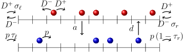
Figure 1: Example of two coupled lattice gases in contact with reservoirs – Model I. The occupancies of sites $i$ of the lower and upper lattices are denoted by $\tau_{i}$ and $\sigma_{i}$, respectively. The bottom lattice has at most one particle per site and the particles can only jump to the right, at rate $p$ (totally asymmetric exclusion dynamics). On the upper lattice, particles hop freely to the right with rate $D^{+}$ and to the left with rate $D^{-}$ (biased diffusive dynamics). Particles on the bottom lattice hop with rate $d$ to the upper lattice whereas those from the upper lattice hop with rate $a$ to empty sites of the lower lattice. Both lattices are coupled to reservoirs with densities $\tau_{\ell},\sigma_{\ell}$ and $\tau_{r},\sigma_{r}$ at their left and right ends, respectively.

2.2 Mean-field equation

To analyze the phase diagram of driven diffusive systems, it is often sufficient to consider a simple mean-field approximation, wherein one replaces the $n$-point correlation function by the product of $n$ one-point correlation functions. For the average occupancies, one then ends up with equations of the form

$$\dot{\tau}_{i}=-{\cal J}^{\tau}_{i}+{\cal J}^{\tau}_{i-1}+K_{i}\;;\qquad\dot{\sigma}_{i}=-{\cal J}^{\sigma}_{i}+{\cal J}^{\sigma}_{i-1}-K_{i},$$ (1)

where $\tau_{i}$ and $\sigma_{i}$ are the average occupancies of the lower and upper lanes at site $i$; ${\cal J}^{\tau}_{i}$, ${\cal J}^{\sigma}_{i}$ are the mean-field approximations of the current between sites $i$ and $i+1$ along the lower and upper lanes, respectively. On the boundaries, the occupancies of both lanes equal those of the reservoirs, $\tau_{l},\sigma_{l}$ and $\tau_{r},\sigma_{r}$ (see figure 1). $K_{i}$ represents the mean-field value of the transverse currents between the two lanes.

For Model I (see figure 1) the currents are given by

$${\cal J}^{\tau}_{i}=p\tau_{i}(1-\tau_{i+1})$$

$${\cal J}^{\sigma}_{i}=D^{+}\sigma_{i}-D^{-}\sigma_{i+1}$$

$$K_{i}=-d\tau_{i}+a\sigma_{i}(1-\tau_{i}).$$ (2)

Although our approach could be carried out at the level of spatially discrete equations (1), it is convenient to take the continuum limit as detailed below.

2.3 Continuum limit

We take the continuum limit and keep terms up to second order in gradients. The mean-field equations are then given by

$$\dot{\tau} = -\partial_{x}[J_{\tau}-D_{\tau}\partial_{x}\tau]+K(\tau,\sigma)$$ (3)

$$\dot{\sigma} = -\partial_{x}[J_{\sigma}-D_{\sigma}\partial_{x}\sigma]-K(\tau,\sigma).$$

Here we have explicitly separated the mean field currents ${\cal J}_{\tau}$ and ${\cal J}_{\sigma}$ into their advective parts, $J_{\tau}$ and $J_{\sigma}$, and their diffusive parts, $-D_{\tau}\partial_{x}\tau$ and $-D_{\sigma}\partial_{x}\sigma$. The advective currents $J_{\tau}$ and $J_{\sigma}$ are non-zero only when the dynamics on the corresponding lane are driven or equivalently when the hopping rates are asymmetric. Equations (3) have to be complemented with boundary conditions on the values of $\sigma$ and $\tau$ which are imposed by the reservoirs:

$$\qquad\tau(0)=\tau_{l}\qquad\tau(L)=\tau_{r}\qquad\sigma(0)=\sigma_{l}\qquad\sigma(L)=\sigma_{r}.$$ (4)

Following assumption (4) we take the boundary densities to be equilibrated, that is

$$K(\tau_{\ell},\sigma_{\ell})=K(\tau_{r},\sigma_{r})=0\;.$$ (5)

We discuss the general case where (5) does not hold in B.2.

Our assumption (3) about the hopping rates between the two lanes made in the previous section amounts to

$$\partial_{\tau}K<0<\partial_{\sigma}K\;.$$ (6)

That is, the transverse current $K$ increases and decreases with the occupancies of the departing and arriving sites, respectively.

In the case of Model I (figure 1), it is straightforward to deduce the currents from Eq. 2

$$J_{\tau} = p\tau(1-\tau)$$ (7)

$$J_{\sigma} = v\sigma$$

$$K = a\sigma(1-\tau)-d\tau\;.$$

Here $v=D^{+}-D^{-}$, $D_{\tau}=p/2$ and $D_{\sigma}=(D^{+}+D^{-})/2$ and we set the lattice constant to unity. Thus, when $D^{+}=D^{-}$, $v=0$ and the model reduces to that of [19]. Also note that $J_{\tau}=J_{\tau}(\tau)$ and $J_{\sigma}=J_{\sigma}(\sigma)$, which is consistent with assumption (2), and that this choice of $K$ satisfies condition (6).

3 Stability analysis

Constant (i.e. flat) profiles $\tau(x)=\tau_{0}$ and $\sigma(x)=\sigma_{0}$ are solutions of the bulk equations (3) as long as they satisfy

$$K(\tau_{0},\sigma_{0})=0.$$ (8)

We refer to such constant solutions as equilibrated plateaux. Because of our assumption (6) on the dependence of $K$ on $\tau$ and $\sigma$, the relation $K(\tau_{0},\sigma_{0})=0$ implies that $\sigma_{0}$ is an increasing function of $\tau_{0}$. Since the hopping rate within each lane does not depend on the occupancy of the other lane – see assumption (ii) – one can show that such solutions are dynamically stable. The details are left to A where it is shown that perturbations about the plateaux $\delta\tau(x,t)=\tau(x,t)-\tau_{0}$ and $\delta\sigma(x,t)=\sigma(x,t)-\sigma_{0}$ decay exponentially in time. On the other hand, we provide in section (6) an example of a more general two-lane system where assumption (ii) does not hold and where equilibrated plateaux are not necessarily dynamically stable.

Let us now consider the steady-state version of the mean-field equations (3)

$$\partial_{x}(D_{\tau}\partial_{x}\tau)=\partial_{x}J_{\tau}(\tau)-K(\tau,\sigma)$$ (9)

$$\partial_{x}(D_{\sigma}\partial_{x}\sigma)=\partial_{x}J_{\sigma}(\sigma)+K(\tau,\sigma)$$ (10)

along with the boundary conditions (4). Generally, constant profiles will not satisfy the boundary conditions (4) on both sides since the left and right reservoirs may impose different densities. It is thus natural to ask whether one can construct steady-state profiles by matching two sets of plateaux that separately satisfy the left and right boundary conditions. As we now show, answering this question requires the study of the spatial stability of perturbations around the plateaux. We refer to perturbations as diverging if they grow as $x$ increases and converging if they decrease as $x$ increases and we refer to the corresponding plateaux as stable or unstable. It is important to note that from now on, any reference to stability or instability has to be understood with reference to the spatial dependence of a profile on $x$, since plateaux are always dynamically stable.

In the example presented in figure 2, for instance, one needs the profiles to diverge away from the left plateaux and converge into the right ones as $x$ increases. Since $\sigma$ is an increasing function of $\tau$ in equilibrated plateaux, the perturbations for $\tau$ and $\sigma$ away from the boundary plateaux must be of the same sign .

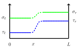
Figure 2: Plateaux imposed by the ‘equilibrated’ densities of left and right reservoirs are simple steady-state solutions of the mean-field equations at both ends of the system. It remains to be known whether the connecting shock is an acceptable steady-state solution.

To check that this indeed can happen we carry out a stability analysis of Eq. (9) and (10). Consider a small perturbation $(\epsilon(x),\eta(x))$ around equilibrated plateaux so that $\tau(x)=\tau_{0}+\epsilon(x)$ and $\sigma(x)=\sigma_{0}+\eta(x)$ where $\tau_{0}$ and $\sigma_{0}$ satisfy $K(\tau_{0},\sigma_{0})=0$. Expanding the steady-state mean-field equations to first order in $\epsilon,\,\eta$ gives

$$D_{\tau}\partial_{x}^{2}\epsilon=(\partial_{\tau}J_{\tau})\partial_{x}\epsilon-(\partial_{\sigma}K)\eta-(\partial_{\tau}K)\epsilon$$ (11)

$$D_{\sigma}\partial_{x}^{2}\eta=(\partial_{\sigma}J_{\sigma})\partial_{x}\eta+(\partial_{\sigma}K)\eta+(\partial_{\tau}K)\epsilon.$$

Here the derivatives with respect to $\tau$ and $\sigma$ are taken at $\tau_{0}$ and $\sigma_{0}$ respectively and similarly $D_{\tau}$ and $D_{\sigma}$ are evaluated at $\tau_{0}$ and $\sigma_{0}$ respectively. Looking for solutions of this system of two second order linear differential equations of the form

$$(\epsilon(x),\eta(x))=\exp(\lambda x)(\epsilon_{0},\eta_{0}),$$ (12)

equations (11) become

$$0=\text{\footnotesize $\pmatrix{\lambda^{2}D_{\tau}-\lambda\partial_{\tau}J_{\tau}+\partial_{\tau}K&\partial_{\sigma}K\cr-\partial_{\tau}K&\lambda^{2}D_{\sigma}-\lambda\partial_{\sigma}J_{\sigma}-\partial_{\sigma}K\cr}$ }\text{\footnotesize $\pmatrix{\epsilon_{0}\cr\eta_{0}\cr}$ }.$$ (13)

For non-trivial solutions to exist, one needs the determinant of the matrix in (13) to vanish, that is

$$\lambda\,\chi(\lambda)=0$$ (14)

where

$$\chi(\lambda) = D_{\tau}D_{\sigma}\lambda^{3}-\lambda^{2}(D_{\tau}\partial_{\sigma}J_{\sigma}+D_{\sigma}\partial_{\tau}J_{\tau})+\lambda(\partial_{\sigma}J_{\sigma}\,\partial_{\tau}J_{\tau}$$

$$+D_{\sigma}\partial_{\tau}K-D_{\tau}\partial_{\sigma}K)+\partial_{\sigma}K\,\partial_{\tau}J_{\tau}-\partial_{\tau}K\,\partial_{\sigma}J_{\sigma}\;.$$

The spatial stability of the plateaux is then determined by the four solutions of the polynomial equation (14). In B we prove that the four solutions, which we denote $\lambda_{0}$, $\lambda_{1}$, $\lambda_{2}$, $\lambda_{3}$, are real and have the following properties:

• There is a trivial solution $\lambda_{0}=0$ which corresponds to shifting the values of the two plateaux while keeping $K=0$, i.e. $(\epsilon_{0},\eta_{0})\propto(-\partial_{\sigma}K,\partial_{\tau}K)$;

• There is exactly one additional solution such that $\epsilon_{0}\eta_{0}>0$. The corresponding root $\lambda_{1}$ is the only root that may change sign as the parameters $(\tau_{0},\sigma_{0})$ are varied and its sign is given by the sign of $\chi(0)$.

• There are two roots $\lambda_{2}<0$ and $\lambda_{3}>0$ with $\epsilon_{0}\eta_{0}<0$.

• The root $\lambda_{1}$ is the only root of (14) relevant for the derivation of the phase diagram: it controls the convergence of perturbations away from constant densities.

• The roots $\lambda_{2}$ and $\lambda_{3}$ only play a role for the boundary layers connecting the plateaux to non-equilibrated reservoirs (i.e. with $K\neq 0$ at the boundary) and not for the construction of the phase diagram (see B.2).

The perturbations $(\epsilon,\eta)$ associated to $\lambda_{1}>0$ thus grow as $x$ increases (a diverging perturbation), while those associated to $\lambda_{1}<0$ decrease (a converging perturbation). From equation (3) it readily follows that the change of spatial stability occurs when

$$\chi(0)=\partial_{\sigma}K(\tau_{0},\sigma_{0})\partial_{\tau}J_{\tau}(\tau_{0})-\partial_{\tau}K(\tau_{0},\sigma_{0})\partial_{\sigma}J_{\sigma}(\sigma_{0})=0.$$ (16)

Thus the perturbations $(\epsilon,\eta)$ grow or decrease with $x$ when $\chi(0)$ is negative or positive, respectively (see B.1).

The method of constructing the phase diagram is then to determine the sign of $\chi(0)$ for each set of equilibrated plateaux (imposed by the boundaries) and deduce whether the plateaux can be connected by appropriate perturbations. For example, the scenario presented in figure 2 requires a diverging perturbation from the left plateau and a converging perturbation at the right plateau. This can only take place if $\chi(0)>0$ for the left plateau densities $\tau_{l}$, $\sigma_{l}$ and $\chi(0)<0$ for the right ones $\tau_{r}$, $\sigma_{r}$. As we illustrate below, this line of reasoning provides a straightforward method to construct the phase diagram of multilane systems.

Before turning to derive the phase diagram for several examples, let us show that $\chi(0)$ is simply related to the derivative of the total current. In equilibrated plateaux, $\sigma_{0}$ and $\tau_{0}$ are related through $K(\tau_{0},\sigma_{0})=0$. The advective part of the total current, defined as

$$J_{\rm tot}=J_{\tau}+J_{\sigma}\;,$$ (17)

may thus be expressed as a function of $\tau_{0}$ whose total derivative is given by

$$\frac{{\rm d}}{{\rm d}\tau_{0}}J_{\rm tot}\big{(}\tau_{0},\sigma_{0}(\tau_{0})\big{)}=\partial_{\tau_{0}}J_{\rm tot}+\partial_{\sigma_{0}}J_{\rm tot}\frac{\partial\sigma_{0}}{{\partial\tau_{0}}}=\partial_{\tau_{0}}J_{\tau_{0}}-\partial_{\sigma_{0}}J_{\sigma_{0}}\frac{\partial_{\tau_{0}}K}{\partial_{\sigma_{0}}K}.$$ (18)

Equation (16) then implies

$$\chi(0)={\partial_{\sigma_{0}}K}\ \frac{{\rm d}J_{\rm tot}}{{\rm d}\tau_{0}}.$$ (19)

Since under our assumptions (see Eq. (6)) $\partial_{\sigma_{0}}K>0$, the sign of $\chi(0)$ is the same as that of $\frac{{\rm d}J_{\rm tot}}{{\rm d}\tau_{0}}$. Therefore, the perturbation connecting different plateaux changes stability at an extremum of the advective part of the total current $J_{\rm tot}$. It is converging when $\frac{{\rm d}J_{\rm tot}}{{\rm d}\tau_{0}}<0$ and diverging when $\frac{{\rm d}J_{\rm tot}}{{\rm d}\tau_{0}}>0$.

Note that the case $\frac{{\rm d}J_{\rm tot}}{{\rm d}\tau_{0}}=0$ requires a special treatment. Maximal current plateaux (where $\frac{{\rm d}^{2}J_{\rm tot}}{{\rm d}\tau_{0}^{2}}<0$) are such that negative perturbations are diverging whereas positive perturbations are converging, so that profiles connected to these plateaux are always decreasing. Conversely, minimal current phases correspond to increasing profiles, i.e. $\tau(x)$ and $\sigma(x)$ increasing with $x$.

4 Construction of the phase diagram – a simple case

To demonstrate how the stability analysis described above can be used to construct phase diagrams of different microscopic models we first study Model I when $D^{+}=D^{-}$ and thus $v=0$ (symmetric diffusion). Later we also consider the more general case where $v\neq 0$.

Using equations (7) and (19), we see that the stability of the equilibrated plateau is set by the sign of

$$\frac{{\rm d}J_{\rm tot}}{{\rm d}\tau_{0}}=p(1-2\tau_{0}).$$ (20)

This example is particularly simple because the advective part of the total current does not depend on $\sigma_{0}$. Equation (20) implies that profiles with $\tau_{0}<1/2$ are diverging (growing with $x$) whereas profiles with $\tau_{0}>1/2$ are converging (decreasing with $x$). The case $\tau_{0}=1/2$ is marginal: negative perturbations are diverging whereas and positive perturbations are converging. This is consistent with our claim, in the previous section, that maximal profiles correspond to $\tau(x)$ and $\sigma(x)$ decreasing with $x$. The different profiles are illustrated in figure 3.

         

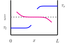
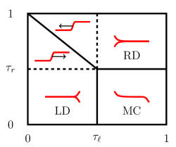
Figure 3: Left: The left and right reservoirs impose boundary densities $\tau_{\ell}$ and $\tau_{r}$. Various possible steady profiles are presented, together with their stability. Right: Phase diagram constrained by the stability of the equilibrated plateaux presented on the left panel.

The construction of the phase diagram is now straightforward. To do this we consider all possible matchings, four in total, between the different stability regions for left and right boundary plateaux.

• When $\tau_{\ell}>1/2$ and $\tau_{r}<1/2$, the only profile consistent with the stability analysis is flat at $\tau(x)=1/2$ connecting to the boundaries at the ends of the system. This corresponds to the maximal current phase (MC phase).

• When $\tau_{\ell}<1/2$ and $\tau_{r}<1/2$, the only profile allowed by the stability analysis is a flat plateau with $\tau(x)=\tau_{\ell}$ and a short boundary layer connecting to the right boundary density (LD phase).

• When $\tau_{\ell}>1/2$ and $\tau_{r}>1/2$, similarly to the previous case, we have $\tau(x)=\tau_{r}$ and a short boundary layer connecting to the left boundary density (RD phase).

• When $\tau_{\ell}<1/2$ and $\tau_{r}>1/2$, the stability analysis is consistent with a shock profile connecting $\tau(x)=\tau_{\ell}$ to $\tau(x)=\tau_{r}$. The velocity of the shock, $v_{s}=(J_{\tau}(\tau_{\ell})-J_{\tau}(\tau_{r}))/(\tau_{r}-\tau_{\ell})$ is given by mass conservation. Therefore, the shock is steady for $\tau_{r}=1-\tau_{\ell}$ and is localized on the right or the left boundary for $\tau_{r}>1-\tau_{\ell}$ and $\tau_{r}<1-\tau_{\ell}$ respectively.

The corresponding phase diagram is drawn in figure 3 and is consistent with the results presented in [19]. This phase diagram reduces to that of the TASEP because of the lack of bias on the diffusive lane. In effect the diffusive lane adjusts its density to ensure that there is zero transverse flux between the lanes, therefore the phase diagram is determined by that of the driven lane i.e. the TASEP.

5 Two-lane models with non-trivial phase diagrams

In this section we consider more general two-lane systems which exhibit non-trivial phase diagrams. In these cases the phase diagrams are much richer than the TASEP coupled to a symmetric diffusive lane considered in the previous section, and we analyse in detail the phase diagrams of several such examples.

5.1 TASEP and biased diffusion

In this subsection we consider a TASEP coupled to a biased diffusive lane which corresponds to $v>0$ in Model I. Such a model is relevant to a biophysical situation where molecular motors diffuse asymmetrically after detaching from protofilaments, as for instance in models of cooperative extraction of membrane tubes [23].

Let us first show that in the presence of a bias in the diffusive lane, the phase diagram of Model I can become more complex and exhibit several new phases. As explained in section 3, the phase diagram can be deduced from ${\rm d}J_{\rm tot}/{\rm d}\tau_{0}$. From the continuous mean-field equations (3) and (7), one obtains

$$J_{\rm tot}=p\tau(1-\tau)+v\sigma.$$ (21)

For equilibrated plateaux, $K=0$ imposes

$$\sigma_{0}=\frac{d}{a}\frac{\tau_{0}}{1-\tau_{0}},$$ (22)

so that

$$J_{\rm tot}(\tau_{0})=\frac{vd}{a}\frac{\tau_{0}}{1-\tau_{0}}+p\tau_{0}(1-\tau_{0}).$$ (23)

The values of $\tau_{0}$ where the stability changes are given by  ${\rm d}J_{\rm tot}(\tau_{0})/{\rm d}\tau_{0}=0$ which reads

$$(1-2\tau_{0})(\tau_{0}-1)^{2}=-\frac{vd}{pa}.$$ (24)

Simple algebra shows that this equation always has an unphysical root at $\tau_{0}>1$. Furthermore, one can distinguish two regimes, according to the value of $vd/pa$, which exhibit distinct phase diagrams as we now discuss.

Regime $v>pa/27d$: in this case there are no physical roots of equation (24). One finds that the plateaux are always diverging. Since all profiles are diverging, there is only one phase. One only observes a plateau with a density given by the density at the left boundary and a small boundary layer that connects to the right boundary. In this regime the advection in the diffusive lane is sufficiently strong that the left boundary always dominates.

Regime ${pa}/27d>v>0$: in this case there are two roots of (24), denoted $\tau_{M}$ and $\tau_{m}$, which lie between 0 and 1. Therefore the stability of the plateau changes twice: it is diverging for $\tau_{0}$ close to 0 and 1 and is converging in the intermediate region (see figure 4). The smallest root $\tau_{M}$ is a local maximum of $J_{\rm tot}(\tau_{0})$, so that profiles that are connected to the corresponding plateau are decreasing. On the contrary, the plateau at $\tau_{m}$ can only be connected to increasing profiles (see figure 4).

We now illustrate how the phase diagram can be constructed using figure 4. Once again, we look at possible matchings of the plateaux imposed by the boundary conditions. Both $\tau_{\ell}$ and $\tau_{r}$ can be in the three different regions separated by $\tau_{M}$ and $\tau_{m}$. As indicated in figure 4, each of these nine cases has to be analyzed separately and the result is five distinct phases for any $d,a\neq 0$. Two of the phases disappear at $d=0$.

1. Regions $R(i)$, $L(i)$ and $L^{\prime}(i)$: if the left and right densities are in the same stability region (a total of 3 different possibilities) there is one plateau set by one boundary and a small boundary layer that connects to the other boundary. For diverging regions ($\tau_{r},\tau_{\ell}<\tau_{M}$ and $\tau_{r},\tau_{\ell}>\tau_{m}$) the left density controls the plateau whereas the right boundary dominates in the converging region ($\tau_{M}<\tau_{r},\tau_{\ell}<\tau_{m}$).

2. Regions $mC(ii)$ and $MC(ii)$: when $\tau_{M}<\tau_{\ell}<\tau_{m}$ and $\tau_{r}<\tau_{M}$, the stability implies a plateau at $\tau_{M}$. Since this value corresponds to a local maximum of the current, we conclude that this region belongs to a maximal current phase. Similarly, when $\tau_{M}<\tau_{\ell}<\tau_{m}$ and $\tau_{r}>\tau_{m}$, the stability implies a plateau at $\tau_{m}$. This region therefore belongs to a minimal current phase.

3. Regions $L(iii)$ and $R(iii)$: when $\tau_{\ell}<\tau_{M}$ and $\tau_{M}<\tau_{r}<\tau_{m}$, the stability analysis predicts that the corresponding plateaux can be connected by an upward shock, from low to high density plateau. Since the total density $\rho=\tau+\sigma$ is locally conserved, the shock velocity is given by

   $$v_{s}=[J_{\rm tot}(\tau_{r})-J_{\rm tot}(\tau_{\ell})]/(\rho_{r}-\rho_{\ell}).$$ (25)

   Here, $\rho_{r}>\rho_{\ell}$ and the plateau associated with the smallest current extends whereas the other recedes. The limiting case $J_{\rm tot}(\tau_{r})=J_{\rm tot}(\tau_{\ell})$ defines a boundary line $\tau_{\ell}(\tau_{r})$ separating a ‘right-dominated’ phase $R(iii)$ from a ‘left-dominated’ one $L(iii)$, corresponding to a discontinuous phase transition. On this line, a shock in the profile can in principle be observed.

4. Regions $L(iv)$ and $mC(iv)$: when $\tau_{\ell}<\tau_{M}$ and $\tau_{r}>\tau_{m}$, the stability analysis predicts that a plateau of density $\tau_{\ell}$ can be connected by a shock to a plateau of density $\tau_{m}$ which is then connected to the right density through a small boundary layer. This phase can be either ‘left-dominated’ or in a minimal current phase depending on the sign of the shock velocity. Since the shock is upward, the plateau with the lowest current dominates. A shock can in principle be observed on the transition line where $J_{\rm tot}(\tau_{\ell})=J_{\rm tot}(\tau_{m})$.

5. Regions $L(v)$ and $R(v)$: when $\tau_{\ell}>\tau_{m}$ and $\tau_{M}<\tau_{r}<\tau_{m}$ the stability analysis allows a downward shock to form in the system. Similar to the arguments regarding shocks presented above since $\rho_{\ell}>\rho_{r}$ the plateau associated with the larger current controls the system. The phase transition line is given by $J_{\rm tot}(\tau_{r})=J_{\rm tot}(\tau_{\ell})$.

6. Regions $L(vi)$ and $MC(vi)$: when $\tau_{\ell}>\tau_{m}$ and $\tau_{r}<\tau_{M}$ the stability analysis allows a downward shock to form in the system from $\tau(x)=\tau_{\ell}$ to a lower density given by $\tau_{M}$. The latter is then connected to the right boundary with a short boundary layer. The scenario is depicted in figure 4. Again the larger current controls the system and there is a phase transition when $J_{\rm tot}(\tau_{M})=J_{\rm tot}(\tau_{\ell})$.

Note that the contiguous regions $L(i)$, $L(iii)$, $L(iv)$ are all controlled by the density at the left end of the system and therefore constitute a single, low-density, phase, with plateaux density smaller than $\tau_{M}$. Similarly, the three contiguous phases $L(v)$, $L(vi)$ and $L^{\prime}(i)$ form a single high-density phase, in which the plateau density is larger than $\tau_{m}$. Then, each of the groups of regions [$R(i)$, $R(iii)$, $R(v)$], [$MC(ii)$,$MC(vi)$], [$mC(iv)$, $mC(ii)$] defines a different phase.

To summarize this subsection, we have constructed the phase diagram using a stability analysis. The resulting phase diagram has five distinct phases. In figure 4 the results of the analysis are compared to continuous time Monte-Carlo simulations and shown to agree very well.

Note that we show in C that the above stability analysis leads to the same phase diagram as a generalization of the extremal current principle to the two-lane systems. For increasing profiles ($\tau_{\ell}\leq\tau_{r}$) the steady plateaux are such that $J_{\rm tot}(\tau)$ realizes its minimum for $\tau\in[\tau_{\ell},\tau_{r}]$. Conversely, for decreasing profiles ($\tau_{\ell}>\tau_{r}$), the steady profiles are such that $J_{\rm tot}(\tau)$ realizes its maximum for $\tau\in[\tau_{r},\tau_{\ell}]$. Which of the two methods one chooses to use is thus a matter of convenience.

Next, we derive the phase diagram for two other two-lane models and compare the results to continuous time Monte-Carlo simulations. The derivation follows very similar lines to that presented above and we thus only outline the main differences.

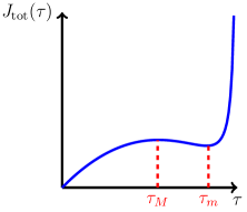
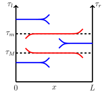
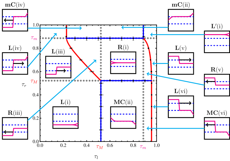
Figure 4: Top-left: Current-density relation for the TASEP coupled to a biased diffusive lane. Top-right This figure represents a side view of steady density profiles that can be used to connect two reservoirs with densities $\tau_{r}$ and $\tau_{l}$. According to the stability analysis, in the steady states, one can get diverging profiles for $\tau\leq\tau^{M}$ or $\tau\geq\tau^{m}$ and converging profiles otherwise. Note that the extremal densities have been spread out for clarity and their values are just illustrative. Bottom: Phase diagram of a TASEP coupled to a biased diffusive lane, for parameters $p=1,\,d=0.01,\,a=1,\,D=1,\,v=1$. The blue and red lines correspond to continuous and discontinuous phase transitions predicted by the theory while the black symbols were obtained from continuous time Monte-Carlo simulations. The grey dotted lines correspond to the local minimum and maximum of $J_{\rm tot}$. Insets illustrate the stability discussion of the main text and the consequent profiles observed in the steady state. $L$ and $R$ stand for left- and right-dominated phase while mC and MC stand for minimal and maximal current phase.

5.2 Two coupled TASEPs with advection in the same direction

In this subsection we consider two coupled TASEPS with advection in the same direction but of different strength in the two lanes.

For two coupled TASEPs with equilibrated boundaries, Harris and Stinchcombe have shown that if the extremal current principle applies, then the phase diagram should be the same as that of a single-lane TASEP with next-nearest neighbours interactions [35]. They backed up this assumption by simulating the profiles for several points in the phase diagram. Here we derive the phase diagram using the stability argument. Our results agree with those found in [35] and with continuous time Monte-Carlo simulations (see figure 6).

The model we study in this subsection is defined as follows. We consider two lanes, each consisting of a one-dimensional lattice with $L$ sites. On the lower lane particles hop to a nearest neighbour empty site to their right with rate $p$. On the upper lane particles hop to a nearest neighbour empty site on the right with rate $q$. In addition particles can hop from site $i$ on the upper lane to an empty site $i$ on the lower lane with rate $a$ and vice versa with rate $d$. To analyze the phase diagram we note that the currents along the two lanes are given by:

$$J_{\tau}=p\tau(1-\tau)\quad;\quad J_{\sigma}=q\sigma(1-\sigma).$$ (26)

Because of the exclusion on both lanes, the transverse current $K$ reads

$$K=a\sigma(1-\tau)-d\tau(1-\sigma).$$ (27)

Using the $K=0$ condition, one can write the total current in an equilibrated plateaux as a function of $\tau_{0}$ as

$$J_{\rm tot}=\tau_{0}(1-\tau_{0})\left(p+q\frac{da}{[a(1-\tau_{0})+d\tau_{0}]^{2}}\right).$$ (28)

The total current as a function of $\tau_{0}$ is shown in figure 5 for the most interesting case in which the curve has three extrema (depending on parameters there is also a less interesting case with only one extrema). This is the scenario we study below.

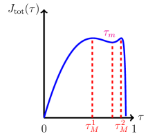
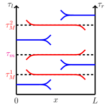
Figure 5: Left: Current density relation for two coupled TASEPs with a bias in the same direction. Right: Sketch of the stability of various steady-state profiles for two coupled TASEPs with a bias in the same direction. Note that the extremal densities have been spread out for clarity and their values are just illustrative.

As before the stability of the plateaux changes when ${\rm d}J_{\rm tot}(\tau)/{\rm d}\tau=0$. As can be inferred from figure 5 there are now three solutions which we denote, from smallest to largest, by $\tau_{M}^{1},\tau_{m}$ and $\tau_{M}^{2}$. These lead to four distinct regimes of stability. When $\tau<\tau_{M}^{1}$ and $\tau_{m}<\tau<\tau_{M}^{2}$ the plateau are diverging and when $\tau_{M}^{1}<\tau<\tau_{m}$ and $\tau>\tau_{M}^{2}$ the plateau are converging. Using a procedure identical to the one outlined above one can readily construct the phase diagram shown in figure 6. For example, consider phase $L$ in the small $\tau_{\ell}$ region. One then notes that for $\tau_{\ell}<\tau_{M}^{1}$ and $\tau_{r}<\tau_{M}^{1}$ there is a plateau controlled by the left boundary with a small boundary layer on the right of the system. When $\tau_{\ell}<\tau_{M}^{1}$ and $\tau_{M}^{1}<\tau_{r}<\tau_{m}$ an upward shock connects the two boundaries. The system is then controlled by the smaller current which is given by $J(\tau_{l})$ up to the line defined by $J(\tau_{\ell})=J(\tau_{r})$ and give rise again to a density controlled by the left boundary. Similarly when $\tau_{\ell}<\tau_{M}^{1}$ and $\tau_{m}<\tau_{r}<\tau_{M}^{2}$ the scenario is identical but with the right plateau at $\tau_{m}$ and a small boundary layer at the right end of the system. Again it is easy to see that the system’s density is controlled by $\tau_{\ell}$ up to the line defined by $J(\tau_{\ell})=J(\tau_{m})$. Finally, when $\tau_{\ell}<\tau_{M}^{1}$ and $\tau_{r}>\tau_{M}^{2}$ the stability analysis allows for two upward shocks. One between $\tau_{\ell}$ and $\tau_{m}$ and one between $\tau_{m}$ and $\tau_{r}$. It is straightforward to see that the plateau with $\tau_{\ell}$ dominates up to the line defined by $J(\tau_{r})=J(\tau_{\ell})$.

The same arguments can easily be extended to construct the rest of the phase diagram shown in figure 6. The $L$ ($R$) phase has a density controlled by the left (right) boundary and $mC$ is a minimal current phase with density $\tau_{m}$. The $MC_{1}$ ($MC_{2}$) phase is a maximal current phase with a density $\tau_{M}^{1}$ ($\tau_{M}^{2}$). Finally, noting that $J(\tau_{M}^{1})=J(\tau_{M}^{2})$ phase $\overline{m}$ corresponds to a shock phase with a density $\tau_{M}^{2}$ on the left of the shock and a density $\tau_{M}^{1}$ on its right. Note that there are two distinct phases controlled by the right boundary, one is a high-density phase in which $\tau_{r}$ is larger than $\tau_{M}^{2}$ whereas the other is intermediate between $\tau_{M}^{1}$ and $\tau_{m}$. Similarly, there are two distinct phases controlled by the left boundary, one with a low density $\tau_{\ell}<\tau_{M}^{1}$ and one with densities intermediate between $\tau_{m}$ and $\tau_{M}^{2}$.

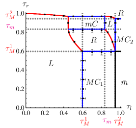
Figure 6: Phase diagram of two forward TASEPs with $p=q=1,\,d=0.04,\,a=1$. The blue and red lines correspond to the continuous and discontinous phase transitions predicted by the stability analysis. The dotted grey line indicate the extrema of the current and the black dots are the results of the continuous time Monte-Carlo simulations.

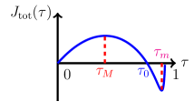
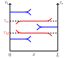
Figure 7: Current density relation, typical stability profiles for 2 TASEPs flowing in opposite directions for $p=q=1$, $d=0.04$ and $a=1$. Note that the extremal densities have been spread out for clarity and their values are just illustrative.

5.3 Two coupled TASEPs with advection in opposite directions

It is natural to look at the phase diagram of two TASEP lattices when the current in each of the lattices is directed in an opposite direction. Specifically we consider the two TASEP model considered above but where now particles on the upper lane hop to nearest neighbour empty sites to their left with rate $q$.

Similarly to the case described above the currents on both lanes are given by

$$J_{\tau}=p\tau(1-\tau);\qquad J_{\sigma}=-q\sigma(1-\sigma),$$ (29)

whereas the transverse current is still given by (27). The $K=0$ condition now yields for the total current $J_{\rm tot}$:

$$J_{\rm tot}=\tau_{0}(1-\tau_{0})\left(p-q\frac{da}{[a(1-\tau_{0})+d\tau_{0}]^{2}}\right).$$ (30)

In what follows we assume $a>d$ (the regime $a<d$ can be obtained by symmetry) and furthermore, to obtain a phase diagram which is significantly different from that of the single lane TASEP, we take $pa/d>q>pd/a$. It is easy to check that when $q$ is outside this range the current has only one extremum. The current in the regime of interest is shown in figure 7. As is evident there are now two points, denoted by $\tau_{M}$ and $\tau_{m}$, where the stability changes. Plateaux are unstable for $\tau<\tau_{M}$ and $\tau>\tau_{m}$ and are stable for $\tau_{M}<\tau<\tau_{m}$.

To construct the phase diagram we use the stability regimes (sketched in figure 7) as discussed above. The results are shown in figure 8. Phases $R$ and $L$ correspond to phases which are controlled by the density of the right and left reservoirs respectively. $MC$ corresponds to a maximal current phase with a density $\tau_{M}$ and the phase $mC$ corresponds to a minimal current phase with a density $\tau_{m}$. It is interesting to note that inside phase $R$, say, as $\tau_{r}$ is increased, the total current in the system changes direction. This, however, happens in a smooth manner and is therefore not associated with a phase transition in the system. Note that as in the previous cases, there are two phases controlled by the left reservoirs, corresponding to low and high density phases ($\tau_{\ell}<\tau_{M}$ and $\tau_{\ell}>\tau_{m}$, respectively).

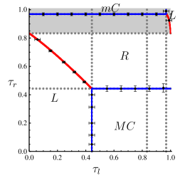
Figure 8: Phase diagram of 2 TASEPs with opposite advection directions. $p=q=1$, $d=0.04$ and $a=1$. The area with a negative current total current is greyed. The dotted grey lines correspond to the extrema of the current while the black dots were obtained from continuous time Monte-Carlo simulations.

6 A counter example—run-and-tumble model

The derivations presented throughout the paper rely on assumption (ii) that the hopping rates of the particles within a lane depend only on the occupancies of their site and neighbouring sites within their lane. In this section we show that when the hopping rates on each lane depend on the occupancies of the others, implying interactions between lanes and a violation of assumption (ii), the situation is more subtle. In particular the results of A, pertaining to the dynamical stability, do not always hold. To see this, below we explicitly look at a specific two-lane model with interactions. We show that in this model the equilibrated plateaux are not dynamically stable and therefore neither our stability analysis nor the extremal current principle hold.

We consider a ‘run and tumble’ model with partial exclusion (see figure 9). Particles at site $i$ of the lower lane hop to the right with rate $d_{i}^{+}$ while those on the upper lane hop to the left with rate $d_{i}^{-}$. To account for partial exclusion the rates $d^{\pm}_{i}$ at which particles hop are given by

$$d_{i}^{\pm}=v^{\pm}\left(1-\frac{\tau_{i\pm 1}+\sigma_{i\pm 1}}{\rho}\right)$$ (31)

These rates decrease with the occupancy of the arrival site and are such that for any site $i$ the total occupancy $\tau_{i}+\sigma_{i}$ is always lower than $\rho$ (which is treated as an external parameter). In addition, particles switch lane (or ‘tumble’) at rate $\alpha/2$.

The symmetric case without reservoirs was studied in [44] where it was shown than flat profiles are unstable at high enough density. The system undergoes phase-separation which results in an alternating profile with low and high density plateaux, separated by domain walls that perform random walks. The presence of advection ($v^{+}\neq v^{-}$) changes this picture slightly. At high enough density, equilibrated plateaux are again unstable and tends to phase separate. But as can be seen in figure 9, the domain walls propagate with non-zero velocity, according to a mass-conservation principle (25).

Equilibrating the plateaux imposes $\tau_{0}=\sigma_{0}$ and the current-density relation is thus very similar to that of the TASEP

$$J(\tau_{0})=(v^{+}-v^{-})\tau_{0}\left(1-\frac{2\tau_{0}}{\rho}\right)$$ (32)

The phase shown in figure 9 has however no counterpart in the TASEP phase diagram, which shows that the extremal current principle does not apply here. In addition, the current carried by the system can be shown to be unequal to the one imposed by the boundaries.

     

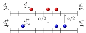
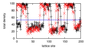
Figure 9: Left: Model of run-and-tumble particles on lattice. The interactions are set by the rates (31). Right: Result of continuous time Monte Carlo simulations for $\alpha=1$, $v^{+}=12$, $v^{-}=8$, $\rho=100$ and a system of $L=200$ sites. Both left and right reservoirs tend to impose plateaux of density $\tau_{0}=\sigma_{0}=26.5$. At $t=0$ the system is prepared with plateaux $\tau_{0}=\sigma_{0}=26$ but these plateaux are unstable and the system phase separates. Two successive snapshots of the total density $\tau_{i}+\sigma_{i}$ are plotted at $t=51$ (black) and $t=71$ (red). This shows the advection of the domain walls.

7 Conclusion

We have introduced a stability analysis which can be used to derive phase diagrams of driven diffusive systems. In particular, we have shown how the method can be applied to a class of two lane models and demonstrated its applicability using several examples. In some of them this allowed us to recover previously derived results with ease; we have also mapped out new phase diagrams for more elaborate models. Furthermore, the method was shown to be equivalent to a extremal current principle and either method can be used according to convenience.

The phase diagrams we have derived reveal some interesting physics. In the case of a totally asymmetric exclusion process (TASEP) coupled to a diffusive lane the phase diagram is unchanged from the single lane TASEP. However when a bias is introduced into the diffusive lane new phases emerge such as a minimal current phase and both low and high density phases controlled by the left boundary (figure 4). Similarly, when a TASEP is coupled to another TASEP a rich phase diagram including two left- and two right-boundary controlled phases, two maximal current phases and a minimal current phase emerges (figure 6). In addition for two coupled TASEPs with currents in opposite directions, a change in the direction of the total current may occur, although there is no associated phase transition (figure 8).

It is important to note that we have also pointed out that the stability analysis, as well as the extremal current method, can fail for a broader class of models than outlined in this paper. For example, it can fail when the motion of particles on one lane is influenced by the motion on the other lane. To apply the method in such cases the dynamical stability of plateaux has to be considered in detail.

Finally, we note that the method can be generalized to classes of multi-lane models. This will be discussed in detail in a future publication.

Appendix A Dynamical Stability of Equilibrated Plateaux

In this appendix we show that for two-lane systems equilibrated plateaux are always dynamically stable provided the hopping rate along one lane does not depend on the occupancy of the other lane (a case ‘without interactions’ between the lanes). As shown in section 6 however, plateaux can be unstable if the aforementioned condition is not satisfied.

Let us consider a perturbation around an equilibrated set of plateaux $(\tau_{0},\sigma_{0})$:

$$\tau(x)=\tau_{0}+\sum_{q}\delta\tau_{q}{\rm e}^{iqx};\qquad\sigma(x)=\sigma_{0}+\sum_{q}\delta\sigma_{q}{\rm e}^{iqx}\;.$$ (33)

At linear order in the perturbations, the Fourier modes decouple and the mean-field equations (3) yield

$$\frac{\rm d}{{\rm d}t}\text{\footnotesize $\pmatrix{\delta\tau_{q}\cr\delta\sigma_{q}\cr}$ }=M\cdot\text{\footnotesize $\pmatrix{\delta\tau_{q}\cr\delta\sigma_{q}}$ };\qquad M=\text{\footnotesize $\pmatrix{-D_{\tau}q^{2}-iqJ_{\tau}^{\prime}+\partial_{\tau}K&\partial_{\sigma}K\cr-\partial_{\tau}K&-D_{\sigma}q^{2}-iqJ_{\sigma}^{\prime}-\partial_{\sigma}K\cr}$ }\;,$$ (34)

where $J_{\tau}^{\prime}=\partial_{\tau}J_{\tau}$ and $J_{\sigma}^{\prime}=\partial_{\sigma}J_{\sigma}$. The plateaux are dynamically stable if the eigenvalues of the matrix $M$ have negative real parts. To see this, for simplicity, we first introduce $a,b,c,d$ such that

$$M=\text{\footnotesize $\pmatrix{a&b\cr c&d\cr}$ }\;.$$ (35)

The eigenvalues $\lambda^{\pm}$ are then given by

$$2\lambda^{\pm}=(a+d)\pm\sqrt{(a-d)^{2}+4bc}\;.$$ (36)

We denote by $R(z)$ and $I(z)$ the real and imaginary part of a complex number $z$, respectively. Note that

$$R(a+d)=-(D_{\tau}+D_{\sigma})q^{2}-\partial_{\sigma}K+\partial_{\tau}K<0\;,$$ (37)

since all the terms are negative. For the real part of $\lambda^{\pm}$ to be negative, it is thus sufficient to have

$$|R(a+d)|>|R(\sqrt{z})|\quad\text{with}\quad z=(a-d)^{2}+4bc\;.$$ (38)

Using the relation

$$R(\sqrt{z})=\sqrt{\frac{R(z)+|z|}{2}}\;$$ (39)

we see that (38) is equivalent to

$$2[R(a+d)]^{2}>R[(a-d)^{2}]+4bc+|z|\;,$$ (40)

since $bc$ is real. Using this, a lengthy but straightforward algebra yields

$$|a-d|^{2}-4bc+8R(a)R(d)>|(a-d)^{2}+4bc|\;.$$ (41)

Furthermore, since

$$R(a)R(d)=D_{\tau}D_{\sigma}q^{4}-\partial_{\tau}K\partial_{\sigma}K+q^{2}(\partial_{\sigma}KD_{\tau}-\partial_{\tau}KD_{\sigma})>-\partial_{\tau}K\partial_{\sigma}K,$$ (42)

we have $8R(a)R(d)>8bc$ and thus

$$|a-d|^{2}-4bc+8R(a)R(d)>|a-d|^{2}+4bc>|(a-d)^{2}+4bc|\;,$$ (43)

where the last inequality is the triangular inequality. Hence, the real parts of the two eigenvalues are negative and the plateau is dynamically stable.

Appendix B Eigenvalues and Eigenvectors of the Stationary Stability Problem

In this appendix we present in more detail the stability of the perturbations around equilibrated plateaux and the role they play for the profiles. We first discuss in subsection B.1 the solution of equation (14)

$$0 =\lambda\,\chi(\lambda)$$ (44)

$$\chi(\lambda) =D_{\tau}D_{\sigma}\lambda^{3}-\lambda^{2}(D_{\tau}\partial_{\sigma}J_{\sigma}+D_{\sigma}\partial_{\tau}J_{\tau})$$

$$\quad+\lambda(\partial_{\sigma}J_{\sigma}\partial_{\tau}J_{\tau}+D_{\sigma}\partial_{\tau}K-D_{\tau}\partial_{\sigma}K)$$

$$\quad+\partial_{\sigma}K\partial_{\tau}(J_{\tau})-\partial_{\tau}K\partial_{\sigma}(J_{\sigma}),$$

that controls the increase or decrease of the perturbations $(\epsilon,\eta)={\rm e}^{\lambda x}(\epsilon_{0},\eta_{0})$ that satisfy

$$0=\text{\footnotesize $\pmatrix{\lambda^{2}D_{\tau}-\lambda\partial_{\tau}J_{\tau}+\partial_{\tau}K&\partial_{\sigma}K\cr-\partial_{\tau}K&\lambda^{2}D_{\sigma}-\lambda\partial_{\sigma}J_{\sigma}-\partial_{\sigma}K\cr}$ }\cdot\text{\footnotesize $\pmatrix{\epsilon_{0}\cr\eta_{0}\cr}$ }.$$ (46)

We then discuss in subsection B.2 the stability analysis near non-equilibrated reservoirs.

B.1 Eigenvalues

First, one of the roots of (44) is a trivial $\lambda=0$ solution. The corresponding perturbation satisfies

$$(\epsilon_{0},\eta_{0})\propto(-\partial_{\sigma}K,\partial_{\tau}K).$$ (47)

Such perturbation corresponds to shifting the values of the two plateaux while keeping $K=0$. Indeed, one can readily check that

$${\rm d}K(\tau,\sigma)=\partial_{\tau}K\epsilon_{0}+\partial_{\sigma}K\eta_{0}\propto-\partial_{\tau}K\partial_{\sigma}K+\partial_{\sigma}K\partial_{\tau}K=0.$$ (48)

We now show that there is only one solution $(\epsilon_{0},\eta_{0})$ of equation (46) that satisfies $\epsilon_{0}\eta_{0}>0$. To see this, we sum the two rows of equation (46) and divide by $\lambda$ to get

$$\lambda=\frac{D_{\tau}\epsilon_{0}}{D_{\tau}\epsilon_{0}+D_{\sigma}\eta_{0}}A+\frac{D_{\sigma}\eta_{0}}{D_{\tau}\epsilon_{0}+D_{\sigma}\eta_{0}}B,$$ (49)

where

$$A=\frac{\partial_{\tau}J_{\tau}}{D_{\tau}}\qquad\mbox{and}\qquad B=\frac{\partial_{\sigma}J_{\sigma}}{D_{\sigma}}.$$ (50)

If $\epsilon_{0}$ and $\eta_{0}$ have the same sign, $\lambda$ has to lie between $A$ and $B$. One however notes that

$$\chi(A)=(A-B)D_{\sigma}{\partial_{\tau}K};\qquad\chi(B)=(A-B)D_{\tau}{\partial_{\sigma}K}.$$ (51)

Since $\partial_{\tau}K<0$ and $\partial_{\sigma}K>0$, one then has that

• if $A>B$, $\chi(A)<0$ and $\chi(B)>0$

• if $A<B$, $\chi(A)>0$ and $\chi(B)<0$,

and thus $\chi({\rm min}(A,B))>0$ and $\chi({\rm max}(A,B))<0$. Since the coefficient of $\lambda^{3}$ in $\chi(\lambda)$ is positive, there is only one root lying between $A$ and $B$ (see figure 10). Since all this requires $\eta_{0}$ and $\epsilon_{0}$ to be of the same sign, this means that there is only one root corresponding to such a perturbation, thus completing our proof.

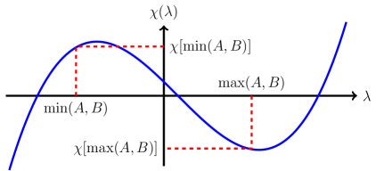
Figure 10: Schematic plot of $\chi(\lambda)$. There is at most one root between $A$ and $B$.

Note that for a marginal perturbation ($\lambda=0$) to exist one needs $\chi(0)=0$, i.e.

$$\partial_{\sigma}K(\tau_{0},\sigma_{0})\partial_{\tau}J_{\tau}(\tau_{0})-\partial_{\tau}K(\tau_{0},\sigma_{0})\partial_{\sigma}J_{\sigma}(\sigma_{0})=0.$$ (52)

This requires that $A$ and $B$ have opposite signs and thus the root that has vanished lies between $A$ and $B$. This means that the only root that can change sign is associated with $\epsilon_{0}\,\eta_{0}>0$.

We now consider the two other roots corresponding to $\epsilon_{0}\eta_{0}<0$. They obey (see figure 10) $\lambda_{2}<{\rm min}(A,B)$ and $\lambda_{3}>{\rm max}(A,B)$. If $AB<0$ then clearly $\lambda_{2}<0$ and $\lambda_{3}>0$. In the case $AB>0$ we consider

$$\chi(0)=D_{\tau}A\partial_{\sigma}K-D_{\sigma}B\partial_{\tau}K\;.$$ (53)

If $A>0$ and $B>0$, then $\lambda_{1}>0$ and $\lambda_{3}>0$ and, from (53), $\chi(0)>0$. Since $\chi(0)$ equals minus the product of the three roots of the cubic equation $\chi(\lambda)=0$, we deduce that $\lambda_{2}<0$. Similarly, if $A<0$ and $B<0$, we have $\lambda_{1}<0$ and $\lambda_{2}<0$. Then $\chi(0)<0$ implies $\lambda_{3}>0$. Thus, in all cases $\lambda_{2}<0$ and $\lambda_{3}>0$ and the sign of $\chi(0)$ equals that of $\lambda_{1}$.

B.2 Connecting equilibrated plateaux to non-equilibrated reservoirs

In this section we show that the perturbations that satisfy $\eta_{0}\epsilon_{0}<0$ play a crucial role in the boundary layers that connect equilibrated plateaux to non-equilibrated reservoirs.

Let us consider the situation presented in figure 11.

Figure 11: Schematic representation of the system

The solution of the non-linear mean-field equations would lead to relations between plateau and reservoir densities

$$\tau^{P}=H_{1}(\tau^{R},\sigma^{R})\quad;\quad\sigma^{P}=H_{2}(\tau^{R},\sigma^{R})\;,$$ (54)

where the $R(P)$ superscript denotes densities at the reservoir (plateau). Since the plateaux densities are equilibrated, $H_{1}$ and $H_{2}$ satisfy $K(H_{1},H_{2})=K(\rho_{1}^{P},\rho_{2}^{P})=0$. Considering arbitrary perturbations $\delta\tau^{R}$ and $\delta\sigma^{R}$, the equilibrium condition $(K=0)$ imposes

$$0=\delta\rho_{1}^{R}[\partial_{\rho_{1}^{P}}K\partial_{\rho_{1}^{R}}H_{1}+\partial_{\rho_{2}^{P}}K\partial_{\rho_{1}^{R}}H_{2}]+\delta\rho_{2}^{R}[\partial_{\rho_{1}^{P}}K\partial_{\rho_{2}^{R}}H_{1}+\partial_{\rho_{2}^{P}}K\partial_{\rho_{2}^{R}}H_{2}]$$ (55)

Since this has to hold for any perturbation, one gets

$$\partial_{\rho_{1}^{P}}K\partial_{\rho_{1}^{R}}H_{1}+\partial_{\rho_{2}^{P}}K\partial_{\rho_{1}^{R}}H_{2} = 0$$ (56)

$$\partial_{\rho_{1}^{P}}K\partial_{\rho_{2}^{R}}H_{1}+\partial_{\rho_{2}^{P}}K\partial_{\rho_{2}^{R}}H_{2} = 0$$ (57)

Last, this linear system of two equations for $\partial_{\rho_{1}^{P}}K$ and $\partial_{\rho_{2}^{P}}K$ has a non-trivial solution only if its determinant vanishes, which requires:

$${\partial_{\rho_{1}^{R}}H_{1}\partial_{\rho_{2}^{R}}H_{2}-\partial_{\rho_{1}^{R}}H_{2}\partial_{\rho_{2}^{R}}H_{1}=0}\;.$$ (58)

Next we construct a perturbation $\delta\tau^{R},\delta\sigma^{R}$ which is constrained to leave the plateau densities unchanged, namely $H_{1,2}(\tau^{R}+\delta\tau^{R},\sigma^{R}+\delta\sigma^{R})=H_{1,2}(\tau^{R},\sigma^{R})$. This requires

$$0 = \partial_{\tau^{R}}H_{1}\delta\tau^{R}+\partial_{\sigma^{R}}H_{1}\delta\sigma^{R}$$ (59)

$$0 = \partial_{\tau^{R}}H_{2}\delta\tau^{R}+\partial_{\sigma^{R}}H_{2}\delta\sigma^{R}$$ (60)

Again, this linear system admits a non-trivial solution iif the determinant vanishes so that

$$\partial_{\tau^{R}}H_{1}\partial_{\sigma^{R}}H_{2}-\partial_{\tau^{R}}H_{2}\partial_{\sigma^{R}}H_{1}=0\;,$$ (61)

which holds due to Eq. (58). Finally, equations (59) and (60) show that the perturbation one has to look for is of the form

$$(\delta\tau^{R},\delta\sigma^{R})\propto(-\partial_{\sigma^{R}}H_{1},\partial_{\tau^{R}}H_{1})$$ (62)

or equivalently

$$(\delta\tau^{R},\delta\sigma^{R})\propto(\partial_{\sigma^{R}}H_{2},-\partial_{\tau^{R}}H_{2})$$ (63)

This in particular means that $\delta\tau^{R}\delta\sigma^{R}<0$. Close to the left boundaries, such perturbations have to decay when $x$ increases and they correspond to the eigenvector with components of opposite signs that has $\lambda<0$ as discussed in the previous section. Conversely, the same reasoning for the right boundaries leads relevant perturbations with $\delta\tau^{R}\delta\sigma^{R}<0$ and $\lambda>0$. This corresponds to the eigenvector with components of opposite sign and $\lambda>0$ as discussed in the previous section.

Concluding, for general systems with non-equilibrated reservoirs, there are boundary layers connecting the reservoirs to equilibrated bulk plateaux, whose behavior is dictated by the eigenvectors with $\epsilon_{0}\eta_{0}<0$, one for each boundary. The connection between the two plateaux is then dictated by the sign of the remaining eigenvalue, that corresponds to $\epsilon_{0}\eta_{0}>0$.

Appendix C Connection with the Extremal Current Principle

For single lane driven diffusive systems, studies based on domain wall theory have led to the formulation of the ‘extremal current principle’ [17]. In the multilane cases, it is also possible to show that for the transverse current $K$ satisfying condition (6) and in the absence of interactions between the lanes, our stability analysis shows that an ‘extremal current principle’ applies.

Namely, for increasing profiles ($\tau_{\ell}\leq\tau_{r}$) the steady profiles form an equilibrated set of plateaux such that $J_{\rm tot}(\tau)$ realizes its minimum for $\tau\in[\tau_{\ell},\tau_{r}]$. Conversely, for decreasing profiles ($\tau_{\ell}>\tau_{r}$), the steady profiles form an equilibrated set of plateaux such that $J_{\rm tot}(\tau)$ realizes its maximum for $\tau\in[\tau_{r},\tau_{\ell}]$. The demonstration of both assertions being almost identical, we only consider here the increasing case.

There are four cases to consider depending on whether $\tau_{\ell}$ and $\tau_{r}$ correspond to stable or unstable plateaux, that is satisfy $J_{\rm tot}^{\prime}<0$ or $J_{\rm tot}^{\prime}>0$ (here quotes abbreviate total derivative with respect to $\tau$). Maximal current profiles are irrelevant since they correspond to decreasing profiles but minimal current profiles play an important role since they correspond to increasing profiles. When they exist, we denote by $\tau_{m}^{1}$ … $\tau_{m}^{k}$ the densities for which $J_{\rm tot}$ has local maxima.

(i) $J_{\rm tot}^{\prime}(\tau_{\ell})>0$ and $J_{\rm tot}^{\prime}(\tau_{r})>0$.

If $J_{\rm tot}^{\prime}(\tau)$ remains strictly positive on the interval $[\tau_{\ell},\tau_{r}]$, $\tau_{\ell}$ and $\tau_{r}$ are not separated by a minimal current phase and the steady-state profile corresponds to $\tau(x)=\tau_{\ell}$ with a short boundary layer on the right. Since $J_{\rm tot}^{\prime}(\tau)>0$ on $[\tau_{\ell},\tau_{r}]$, the steady-state profile indeed minimize $J_{\rm tot}$ on the interval $[\tau_{\ell},\tau_{r}]$.

If $J_{\rm tot}^{\prime}$ vanishes on $[\tau_{\ell},\tau_{r}]$, the end-points are separated by at least one minimal current phase. A profile consistent with the stability analysis is given by a sequence of plateaux of densities in $\{\tau_{\ell},\tau_{m}^{i}\}$ connected by up-going shocks. Mass conservation – equation (25) – shows that an up-going shock separating two density plateaux propagates towards the plateau with the largest current so that the plateaux with the smallest value of the current spread while the others recede. Since $J_{\rm tot}^{\prime}(\tau_{\ell})>0$ and $J_{\rm tot}^{\prime}(\tau_{r})>0$, the smallest value among $\{J_{\rm tot}(\tau_{\ell}),J_{\rm tot}(\tau_{m}^{i})\}$ is indeed the global minimum of $J_{\rm tot}$ in $[\tau_{\ell},\tau_{r}]$.

(ii) $J_{\rm tot}^{\prime}(\tau_{\ell})>0$ and $J_{\rm tot}^{\prime}(\tau_{r})<0$.

$\tau_{\ell}$ is unstable and $\tau_{r}$ is stable. A profile consistent with the stability analysis is given by a sequence of plateaux of densities in $\{\tau_{\ell},\,\tau_{m}^{i},\,\tau_{r}\}$ connected by up-going shocks. Again, the plateaux with the smallest current spread while the others recede and the observed value of $J_{\rm tot}$ is its global minimum in $[\tau_{\ell},\tau_{r}]$.

(iii) $J_{\rm tot}^{\prime}(\tau_{\ell})<0$ and $J_{\rm tot}^{\prime}(\tau_{r})<0$.

$\tau_{\ell}$ and $\tau_{r}$ are stable. If there are no local minimum in $[\tau_{\ell},\tau_{r}]$, the steady profile is a plateau at $\tau=\tau_{r}$, $J_{\rm tot}^{\prime}$ remains strictly negative in $[\tau_{\ell},\tau_{r}]$ and the current is indeed minimized over $[\tau_{\ell},\tau_{r}]$.

If $J_{\rm tot}^{\prime}$ changes sign, it has to do so at least twice and there are local minima $\tau_{m}^{i}$ between $\tau_{\ell}$ and $\tau_{r}$. A sequence of plateau of increasing densities $\tau(x)\in\{\tau_{m}^{i},\tau_{r}\}$ connected by shocks is consistent with the stability analysis. Again, the plateaux with the lowest current spread while the others recede and the corresponding value of the current is the global minimum of $J_{\rm tot}$ in $[\tau_{\ell},\tau_{r}]$.

(iv) $J_{\rm tot}^{\prime}(\tau_{\ell})<0$ and $J_{\rm tot}^{\prime}(\tau_{r})>0$.

There is at least one minimum $\tau_{m}^{i}$ between $\tau_{\ell}$ and $\tau_{r}$. A sequence of plateau of increasing densities $\tau(x)=\tau_{m}^{i}$ is consistent with the stability analysis. If there are several minima, the plateaux with the lowest value of the current spread while the others recede. Since $J_{\rm tot}^{\prime}(\tau_{\ell})<0$ and $J_{\rm tot}^{\prime}(\tau_{r})>0$, the global minimum of $J_{\rm tot}$ is realized by one of the intermediate minimum and the value of $J_{\rm tot}$ is thus indeed minimized on the whole interval.

This concludes the list of 4 possible cases and shows that the current is always minimized between $\tau_{\ell}$ and $\tau_{r}$. Note that in all the above discussion, the minima of the current can be realized by several densities simultaneously. This leads to the coexistence of several plateaux with different densities.

For decreasing profiles, the discussion is very similar, with two main differences. First minimal current profiles do not play any role while maximal current ones do, since only the latter are decreasing. Then, a downwards shock propagates towards the plateaux with the smallest current, so that the plateaux with the largest current spread.

References

References

- [1] S. Katz, J. Lebowitz and H. Spohn, (1983), Phys. Rev. B 28, 1655
- [2] T. Reichenbach, T. Franosch and E. Frey, (2006), Phys. Rev. Lett. 97, 050603
- [3] C.T. Macdonald, J.H Gibbs, A.C.Pipkin (1968), Biopolymers 6 1
- [4] Y. Aghababaie, G. I. Menon, and M. Plischke (1999), Phys. Rev. E, 59 2578,
- [5] H. Grzeschik, R J Harris and L Santen (2010) Phys. Rev. E 81, 031929
- [6] K.E.P. Sugden, M. R. Evans, W.C.K Poon, N. D. Read. (2007), Phys. Rev. E 75 031909
- [7] M. R. Evans and K. E. P Sugden (2007). Physica A 384 53
- [8] O. Campas, Y. Kafri, K. B. Zeldovich, J. Casademunt, and J.-F. Joanny, 2006 Phys. Rev. Lett. 97, 038101.
- [9] D. Mukamel in Soft and Fragile Matter: Nonequilibrium Dynamics, Metastability and Flow IoP publishing, Bristol (2000)
- [10] B. Schmittmann and R. K. P. Zia, Statistical mechanics of driven diffusive systems, volume 17 of Phase transitions and critical phenomena Academic Press, New York (1995)
- [11] J. Krug, 1991 Phys. Rev. Lett. 67, 1882
- [12] B Derrida, M. R. Evans, V. Hakim, V. Pasquier, 1993 J. Phys. A Math. Gen. 26 1493-1517
- [13] G. Schutz and E. Domany, 1993 J. Stat. Phys. 72, 277
- [14] R. A. Blythe and M. R. Evans, 2007 J. Phys. A Math. Theor. 40 R333-R441
- [15] B Derrida, E Domany D Mukamel, 1992 J. Stat. Phys 69 667
- [16] S. Mukherji and S. M. Bhattacharjee, 2005 J. Phys. A Math. Gen. 38 L285
- [17] V. Popkov and G.M. Schütz, 1999 Europhys. Lett. 48, 257-263
- [18] J. S. Hager, J. Krug, V. Popkov, and G. M. Schutz, 2001 Phys. Rev. E 63, 056110
- [19] S Klumpp and R. Lipowsky, 2003 J. Stat. Phys. 113 233-268
- [20] A. Parmeggiani, T. Franosch, and E. Frey, 2003 Phys. Rev. Lett. 90, 086601
- [21] K. Nishinari, Y. Okada, A. Schadschneider, and D. Chowdhury, 2005 Phys. Rev. Lett. 95, 118101
- [22] P. Greulich, A. Garai, K. Nishinari, A. Schadschneider, and D. Chowdhury, 2007 Phys. Rev. E 75, 041905
- [23] J. Tailleur, M. R. Evans, Y Kafri , 2009 Phys. Rev. Lett. 102 118109 (2009)
- [24] G. Korniss, B. Schmittmann, and R. K. P. Zia, 1999 Europhys. Lett. 45, 431
- [25] B. Schmittmann, J. Krometis, and R. K. P. Zia, 2005 Europhys. Lett. 70, 299-305
- [26] A. Melbinger, T. Reichenback, T. Franosch and E. Frey, cond-mat/1002.3766.
- [27] R. Juhasz, 2007 Phys. Rev. E 76 021117
- [28] R. Jiang, K Nishinari, M-B Hu, Y-H Wu and Q-S Wu, 2009 J. Stat. Phys 136,73
- [29] R. Juhasz, 2010 J. Stat. Mech.: Theor. Exp. P03010
- [30] V. Popkov and I Peschel, 2001 Phys. Rev. E 64, 026126
- [31] V. Popkov and G. M. Schutz, 2003 J. Stat. Phys. 112, 523
- [32] E Pronina and A.B. Kolomeisky, 2004 J. Phys. A Math. Gen. 37 9907-9918
- [33] K Tsekouras and A.B. Kolomeisky, 2008 J. Phys. A Math. Theor. 41 465001
- [34] E Pronina and A.B. Kolomeisky, 2006 Physica A 372 12-21
- [35] R. J. Harris and R. B. Stinchcombe, 2005 Physica A 354 582-596
- [36] T. Reichenbach, T. Franosch and E. Frey, 2007 New J. Phys. 9, 159
- [37] R. Jiang, M-B Hu, Y-H Wu and Q-S Wu, 2008 Phys. Rev. E 77, 041128
- [38] C. Schiffmann, C Appert-Rolland and L. Santen, 2010 J. Stat. Mech: Theor. Exp. P06002
- [39] V Popkov, M Salerno, arxiv:1011.3464 (2010)
- [40] V Popkov and M Salerno, 2004 Phys. Rev. E 69 046103
- [41] D Chowdhury, A Garai and J-S Wang, 2008 Phys. Rev. E 77 050902
- [42] S. Mukherji, 2009 Phys. Rev. E 79 041140
- [43] G. M. Schütz, 2003 J. Phys. A: Math. Gen., 36, R339
- [44] A. G. Thompson, J. Tailleur, M. E. Cates, R. A. Blythe J. Stat. Mech. P02029 (2011)