Social Influencing and Associated Random Walk Models: Asymptotic Consensus Times on the Complete Graph

Abstract

We investigate consensus formation and the asymptotic consensus times in stylized individual- or agent-based models, in which global agreement is achieved through pairwise negotiations with or without a bias. Considering a class of individual-based models on finite complete graphs, we introduce a coarse-graining approach (lumping microscopic variables into macrostates) to analyze the ordering dynamics in an associated random-walk framework. Within this framework, yielding a linear system, we derive general equations for the expected consensus time and the expected time spent in each macro-state. Further, we present the asymptotic solutions of the 2-word naming game, and separately discuss its behavior under the influence of an external field and with the introduction of committed agents.

Individual- or agent-based models provide invaluable tools to investigate the collective behavior and response of complex social systems. These systems typically consists of a large number of individuals interacting through a random and sparse network topology. Despite this non-trivial network topology, it has been demonstrated in many recent examples that unlike in low-dimensional spatially-embedded systems with short-range connections, the collective dynamics in sparse random graphs (with no community structure) exhibit scaling properties very similar to those observed on the complete graph. Therefore, studying fundamental agreement processes on the complete graph can yield insights for the ordering process in more realistic sparse random networks. In this paper we consider two simple individual-based models and develop a mathematical framework which yields asymptotically exact consensus times for large but finite complete graphs of size $N$. In particular, after demonstrating the feasibility of this framework on known examples, we apply it to study two distinct stylized approaches in social influencing: (i) influencing individuals by a global external field (mimicking mass media effects) and (ii) introducing committed individuals with a fixed designated opinion (who can influence others but themselves are immune to influence). In the former case, we find the external field dominates the consensus in the large network-size limit, while in the latter case we find the existence of a tipping point, associated with the disappearance of the metastable state in the opinion space. The results further our understanding of timescales associated with reaching consensus in social networks.

I Introduction

Research on non-equilibrium models for social and opinion dynamics has attracted considerable attention Castelano_RMP2009 ; Galam_IJMPC2008 ; Pan2009 . In this paper we present a method to calculate consensus (or ordering) times for a large class of individual-based models with discrete state-variables on the complete graph of size $N$. The mode of reaching consensus depends on the initial configuration and whether or not the individuals are under the influence of a bias. For example, starting from a configuration of evenly mixed opinions with no bias, these systems can exhibit “coarsening” in which case the consensus time typically diverges with the system size in a power-law fashion Pan2009 ; Krapivksy_PRA1992 ; Krapivsky_PRE1996 ; Ben-Naim1996 ; Dornic_PRL2001 ; Baronchelli2006-2 ; Lu_PRE2008 . On the other hand, initializing the system in one particular opinion and exerting some weak bias favoring another opinion create systems that undergo an “escape” from the meta-stable state Lucomm . For networks of finite size, it is important to characterize the consensus time, i.e. the time until the system fully orders.

Direct simulations of the above behaviors can be time-consuming for large systems and essentially impossible even for moderately-sized systems when the system initially is in a meta-stable configuration, as the escape time can increase exponentially with the system size. The method presented here provides a way to obtain the asymptotic behavior of consensus times, including the cases associated with extremely slow meta-stable escapes. While the method and the results presented here are applicable to the complete graph, consensus times often exhibit the same asymptotic scaling with $N$ in large homogeneous sparse random networks Castelano_PRE2005 ; DallAsta_PRE2006 ; Lu_PRE2008 , hence one can gain some insight how ordering and consensus evolves in realistic social networks.

The Naming Game (NG) first emerged in linguistic modeling of the transition from microscopic local interactions to global consensus in the absence of a global coordinator Pan2009 ; Baronchelli2006-2 ; Steels_1995 . This phenomena of total synchrony or global consensus has general interest and applications such as sensor networks, some aspects of neuro-science models for brain functions and social dynamics. Earlier research in this domain mainly discussed two aspects of this model. One focuses on the relationship between the network topology and the dynamics Baronchelli2006 ; DallAsta2006 ; DallAsta_PRE2006 , the other, in contrast, ignores all the effects of network topology and studies the intrinsic property of the dynamics on the complete graph Baronchelli2006-2 ; Baronchelli_IJMPC2008 . The latter for large network size $N$ (also referred to as mean-field or homogeneous mixing) is what we consider in this paper. We assume here an initial configuration where every agent has a non-empty name list of words. The dynamics on the complete graph is driven by the mean field (in this context referring to the fraction of nodes in each state) rather than the detailed network states (including the states of all the nodes). It naturally leads to a coarse-graining approach by lumping microscopic variables into macro-states. Our paper studies the impact of a global external field (mimicking mass media effects) and of presence of committed agents (who will firmly stick to and convey a designated opinion) on the consensus process.

A point worth mentioning is that the Naming Game constitutes an opinion dynamics model in which in which a node can possess multiple opinions simultaneously. Such models with intermediate states have only recently begun receiving attention Dallasta_2008 ; Vazquez_2010 in statistical physics literature, and we believe that this study is an important contribution to this body of literature.

The paper is organized as follows. In Secs. II and III, we introduce the coarse-graining approach to map models for opinion dynamics on the complete graph to an associated random walk problem, and test our framework through known results for the spontaneous agreement process (without any influencing) Slanina_EPJB2003 ; Sood_PRE2008 ; Castelano_PRE2005 ; Baronchelli_IJMPC2008 ; Castello_EPJB2009 . We derive the equations in a linear-system form for the expected total consensus time and the expected time spent in each macro-state which can be solved in a closed form for the voter model Liggett_1985 ; Castelano_RMP2009 ; Krapivksy_PRA1992 (Sec. II). Then, in Sec. III, we employ the same method for a variation of the Naming Game (NG) with two words Castello_EPJB2009 . Finally, and most importantly, we investigate models for social influencing: we present new asymptotic results and discuss the behavior of the 2-word NG under the influence of an external field (Sec. IV) and in the presence of committed agents (Sec. V). A brief summary is given in Sec. VI.

II Consensus time in the voter model on the complete graph

First, we consider a well studied prototypical model for opinion formation, the voter model Liggett_1985 ; Castelano_RMP2009 ; Krapivksy_PRA1992 . In this model, the evolution of a suitably defined global variable can be easily mapped onto a random-walk problem. Further, the solution of this model is known in all dimensions, including the complete graph, hence our method can be tested.

Given a network of $N$ nodes, with each node in a state chosen from the set of possible opinions $X$, the voter model is defined by the following update rule:

A pair of nodes, a “speaker” and a “listener”, are chosen at random. The listener then changes its state to that of the speaker.

If the set of nodes in the network is denoted by $S$, ($\left|{S}\right|$), then the above rule defines a Markov chain in an $N$ dimensional space $X^{S}$. Under mean field assumption, which is justifiable when dealing with complete graphs, one coarse-graining approach is to take all network states in $X^{S}$ corresponding to the same mean field $\vec{n}=(n_{1},n_{2},...,n_{M})$ as a macrostate, where $n_{i}$ denotes the number of nodes in state $i\in X$ and $M=\left|{S}\right|$. Therefore, the coarse-grained random process is valued in a $M-1$ hyper-plane (since $\sum_{i=1}^{M}n_{i}=N$) in M dimension space. When $M=2$ (2-state voter model), taking $X=\{A,B\}$, the coarse-grained process is on a segment (since $n_{A}+n_{B}=N(n_{A},n_{B}>=0)$), and all macrostates can be represented by a single discrete variable $n_{A}=0,1,...,N$.

In each time step $\Delta n_{A}$, the change of $n_{A}$, is a random variable depends only on current macrostate $n_{A}$. Its possible values and the corresponding events and probabilities are listed Table 1.

Table 1: Update events for the voter model and the associated random walk transition probabilities

speaker	listener	event	$\Delta n_{A}(n_{A})$	probability
A	B	$B\rightarrow A$	1	$(1-{n_{A}\over N}){n_{A}\over N-1}$
B	A	$A\rightarrow B$	-1	${n_{A}\over N}(1-{n_{A}-1\over N-1})$
A	A	unchanged	0	${n_{A}\over N}{n_{A}\over N-1}$
B	B	unchanged	0	$(1-{n_{A}\over N})(1-{n_{A}-1\over N-1})$

Hence, the coarse-grained process of the voter model can be mapped to a random walk in 1-d,

$$n_{A}(T)=n_{A}(0)+\sum_{t=0}^{T-1}\Delta n_{A}(n_{A}(t))\;,$$ (1)

where $n_{A}=0,N$ are two absorbing states.

II.1 First-step analysis of consensus times in the voter model

The expected time before absorption which is the quantity of the most interest can be evaluated by first-step analysis Bremaud . The idea is based on a straight forward statement: The absorption time can be decomposed into two parts, the time steps before and after leaving the current macrostate. The former one is called the residence time $t_{r}(n_{A})$ of the given macrostate $n_{A}$. We denote the expected time before absorption and the expected residence time starting from a specific macrostate $n_{A}$ on complete graphs with $N$ nodes as $\tau(n_{A}|N)$ and $t(n_{A}|N)$, respectively, or simply $\tau(n_{A})$ and $t(n_{A})$ when it is not ambiguous. Then taking expectation of all random variables mentioned in the statement above, we get the following equations:

$$\tau(n_{A}) = E[\mbox{time before leaving $n_{A}$}]+E[\mbox{time before absorption and after leaving $n_{A}$}]$$ (2)

$$= E[t_{r}(n_{A})]+E[E[\mbox{time before absorption and after leaving $n_{A}$}|\mbox{entering new macrostate $n_{A}^{\prime}$}]]$$

$$= t(n_{A})+\frac{\sum_{i=-1,1}P(\Delta n_{A}(n_{A})=i)\tau(n_{A}+i))}{1-P(\Delta n_{A}(n_{A})=0)}\;=\;t(n_{A})+\frac{1}{2}(\tau(n_{A}+1)+\tau(n_{A}-1))\;,$$

where $t(n_{A})$ is given by following argument:

$$t(n_{A}) = \Sigma_{k=1}^{\infty}P(t_{r}(n_{A})=k)k\;=\;\Sigma_{k=1}^{\infty}P(t_{r}(n_{A})\geq k)$$ (3)

$$= \Sigma_{k=1}^{\infty}P(\Delta n_{A}(n_{A})=0)^{k-1}\;=\;{1\over 1-P(\Delta n_{A}(n_{A})=0)}\;=\;{1\over 2{n_{A}\over N}(1-{n_{A}\over N-1})}\;.$$

Defining $\vec{\tau}=(\tau(1),...,\tau(N-1))^{T}$, $\vec{t}=(t(1),...,t(N-1))^{T}$ and using boundary conditions $\tau(0)=\tau(N)=0$, we rewrite Eq. (2) as a linear system:

$$\vec{\tau}=Q\vec{\tau}+\vec{t}\;,$$ (4)

where

$$Q=\left[\begin{array}[]{ccccc}0&{1\over 2}&&&\\ {1\over 2}&\cdot&\cdot&&\\ &\cdot&\cdot&\cdot&\\ &&\cdot&\cdot&{1\over 2}\\ &&&{1\over 2}&0\end{array}\right]_{(N-1)\times(N-1)}\;.$$ (5)

$\tau(n_{A}|N)$ can be solved exactly from this equation in terms of $n_{A}$ and $N$. Define $\delta_{N}^{i}$ as a N-entries column vector in which only the ith entry is non-zero and has value 1. We have:

$$\tau(i|N)=(\delta_{N-1}^{i})^{T}\vec{\tau}\;=\;(\delta_{N-1}^{i})^{T}(I-Q)^{-1}\vec{t}\;=\;\vec{u}\cdot\vec{t}\;,$$ (6)

where $\vec{u}=(u_{1},u_{2},...,u_{j},...,u_{N-1})$ is the solution of equation $(I-Q)^{T}\vec{u}=(\delta_{N-1}^{i})$. Intuitively, $u_{j}$ can be understood as the average number of visits (assuming entering and leaving a macrostate as one visit) of macrostate $n_{A}=j$ before absorption and starting from macrostate $n_{A}=i$. Moreover $T_{j}=u_{j}t_{j}$ is actually the average number of time steps (including self-repeating steps) spent on the macrostate $n_{A}=j$ before absorption. It is quite easy to show that $\tau(n|N)$ is monotonic with respect to $N$. Therefore, in order to obtain the large $N$ behavior of $\tau(n_{A}|N)$ we focus on the case when $N$ is even and always assume $n_{A}(0)=N/2$. In such cases, $\vec{u}=(1,2,3,...,N/2,...3,2,1)^{T}$ and

$$\tau(N/2|N) = \vec{v_{N/2}}\cdot\vec{t}\;=\;2\Sigma_{k=1}^{N/2-1}k{1\over 2(k/N)(1-k/(N-1))}+{N\over 2}2$$ (7)

$$= N(N-1)\Sigma_{k=1}^{N/2-1}{1\over N-1-k}+N\;\approx\;N(N-1)\int_{N/2}^{N-2}{dx\over x}+N$$

$$\approx \ln(2)N(N-1)+N\;.$$

As is the convention for agent-based models in statistical physics, unit time is assumed to consist of $N$ update events. Thus, following this convention, the normalized consensus time is $\tau(N/2|N)/N$ is $\ln(2)N$ to the leading order. This agrees with the scaling behavior obtained previously for the characteristic (relaxation) time of the voter model through a Fokker-Planck Slanina_EPJB2003 ; Sood_PRE2008 approach and through simulations Castelano_PRE2005 . .

Figure 1 shows the comparison of the consensus time from numerical simulations (averaged over 50 runs for each $N$) with the analytical results.

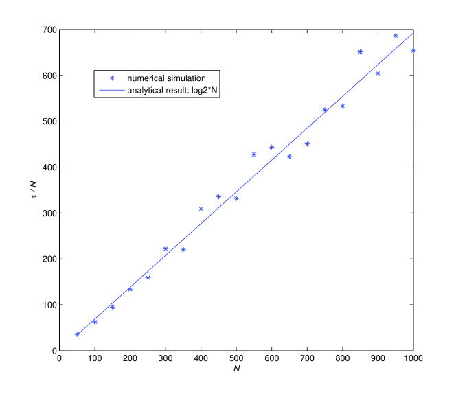
Figure 1: Consensus time for voter model on complete graph. The vertical axis represent the consensus time (normalized by $N$). The horizontal axis is the number of nodes in complete graph. Each star point is an average of 10 runs of numerical simulations of voter model and the solid straight line consists of the solutions of the linear equation for each $N$ value.

III The 2-word Naming Game

The Naming Game (NG) Baronchelli2006 ; Baronchelli_IJMPC2008 ; Castello_EPJB2009 is somewhat more complicated than the voter model because for the given set of all possible opinions (words in the original NG) $X$ $(|X|=M)$, the state of each node is a member of the power set $2^{X}$ - the set of all subsets of $X$ - rather than $X$ itself. Moreover, the update rule is replaced by:

A pair of nodes, a “speaker” and a “listener”, are chosen at random. The speaker then randomly selects one word from her list and communicates it to the listener. If the listener already has this word (termed “successful communication”), she deletes all other words in her list (i.e., collapses her list to this most recently communicated word); If the listener does not have the word communicated by the speaker, she adds it to her list (hence, individuals can carry more than one word at a time).

The slight difference between the update rule defined above and that of the original NG Baronchelli2006 is that here, upon “successful” communication, only the listener changes its state. This restriction eliminates steps of size 2 in the associated RW model, making it easier to apply the method developed in Sec. II.A. Furthermore, we will consider the version of the NG with only two words Castello_EPJB2009 .

The coarse-graining approach mentioned in Section II merges all network states labeled by the same vector $\vec{n}=(n_{i})_{2^{M}-1},i\in 2^{X}\backslash\{\emptyset\}$ into a macrostate. Here $n_{i}$ is the number of nodes in state $i$. The coarse-grained random process takes values in the $2^{M}-2$ hyper-plane: $\sum_{i\in 2^{X}\backslash\{\emptyset\}}n_{i}=N$, thus we can map the coarse-grained process into a $2^{M}-2$ dimension random walk. In the case of 2-word NG $M=2$, so assuming $X=\{A,B\}$, $\vec{n}=(n_{\{A\}},n_{\{B\}},n_{\{A,B\}})$ or $(n_{A},n_{B},n_{AB})$ for short, where $n_{A}$, $n_{B}$, and $n_{AB}$ are the number of individuals carrying word A, word B, or both, respectively. Since $n_{AB}=N-n_{A}-n_{B}$, we dump one redundant dimension and take the 2-d vector $\vec{n}=(n_{A},n_{B})$ to represent the macrostate. In each time step, the change of macrostate $\Delta\vec{n}$ have five possible values. For all these possible values of $\Delta\vec{n}$, the corresponding events and probabilities are listed in Table 2.

Table 2: Update events for the 2-word naming game and the associated random walk transition probabilities

speaker	listener	event	$\Delta\vec{n}(n_{A},n_{B})$	probabilty
B or AB	A	$A\rightarrow AB$	(-1,0)	$P(A-)=n_{A}(N-n_{A}+n_{B})/2N^{2}$
A or AB	AB	$AB\rightarrow A$	(1,0)	$P(A+)=(N-n_{A}-n_{B})(N+n_{A}-n_{B})/2N^{2}$
A or AB	B	$B\rightarrow AB$	(0,-1)	$P(B-)=n_{B}(N+n_{A}-n_{B})/2N^{2}$
B or AB	AB	$AB\rightarrow B$	(0,1)	$P(B+)=(N-n_{A}-n_{B})(N-n_{A}+n_{B})/2N^{2}$
A, B or AB	A or B	unchanged	(0,0)	$P_{0}=(n_{A}+n_{B})/2N+(n_{A}-n_{B})^{2}/2N^{2}$

In Table 2, the event $A\rightarrow AB$, for example, means the listener node changes its state from A to AB. Analogous to the procedure followed for the voter model, we map the coarse-grained 2-word NG to a 2-d random walk,

$$\vec{n}(T)=\vec{n}(0)+\sum_{t=0}^{T-1}\Delta\vec{n}(\vec{n}(t))\;.$$ (8)

Here the domain $D$ of $\vec{n}$ is the set containing all integer grid points bounded by the lines $n_{A}=0$, $n_{B}=0$ and $n_{A}+n_{B}=N$ while $\vec{n}=(0,N),(N,0)$ are two absorbing states. The expected drifts, $E[\Delta\vec{n}(\vec{n})]=(P(A+)-P(A-),P(B+)-P(B-))$ are plotted in Fig. 2 for $N=10$. As shown in Fig. 2, on average, $\vec{n}(t)$ will quickly go to a stable trajectory and then slowly converge to one of the consensus states. In other words, in contrast to an unbiased random walk as in the voter model, the 2-word NG is ”attracted” to the consensus state after a spontaneous symmetry breaking. So it is reasonable to expect that the 2-word NG will achieve consensus much faster than the voter model, both starting from the $n_{A}=n_{B}=N/2$ initial configuration on the complete graph.

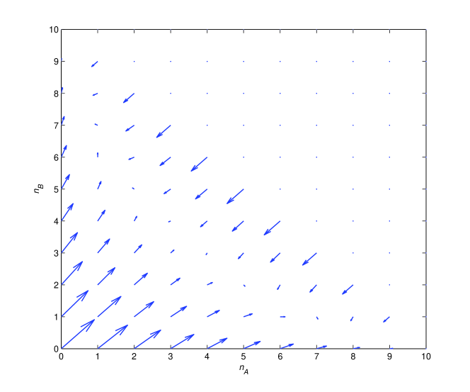
Figure 2: Vector field $E[\Delta\vec{n}(\vec{n})]$ of the random walk coarse-grained from 2-word naming game. Each vector is the expected drift of the random walk at macrostates $\vec{n}$. The network is 10 nodes complete graph and the domain of random walk is the lower triangle of the square lattice

III.1 First-step analysis of consensus times in the 2-word Naming Game

We now repeat the first-step analysis (developed in Sec. II), noting that the method is essentially independent of the number of dimensions. Assume $\tau(\vec{n}|N)$ and $t(\vec{(}n)|N)$ are expected numbers of time steps before absorption and before leaving the current state starting at the macrostate $\vec{n}=(n_{A},n_{B})$, then we have:

$$\tau(\vec{n}) = t(\vec{n})+{\sum_{i\in\{(1,0),(-1,0),(0,1),(0,-1)\}}P(\Delta\vec{n}(\vec{n})=i)\ \tau(\vec{n}+i)\over 1-P(\Delta\vec{n}(\vec{n})=(0,0))}$$ (9)

$$= t(\vec{n})+{P(A+)\tau(n_{A}+1,n_{B})+P(A-)\tau(n_{A}-1,n_{B})+P(B+)\tau(n_{A},n_{B}+1)+P(B-)\tau(n_{A},n_{B}-1)\over 1-P(0)}$$

and

$$t(\vec{n})={1\over 1-P(\Delta\vec{n}(\vec{n})=(0,0))}={1\over 1-(n_{A}+n_{B})/2N-(n_{A}-n_{B})^{2}/2N^{2}}$$ (10)

Ordering all the macrostates $\vec{n}$ (except the two absorbing states) in a vector, and arranging $\tau(\vec{n})$,$t(\vec{n})$ in the same order to get $\vec{\tau}$ and $\vec{t}$ whose dimensions are $(N+2)(N+1)/2-2$, we write the Eq. (9) in the same linear system form $\vec{\tau}=Q\vec{\tau}+\vec{t}$. Furthermore, taking $\delta_{N}^{\vec{n}}$ as a column vector where the only nonzero entry is 1 corresponding to $\vec{n}$, we solve expected number of visits to each macrostate through the equation $(I-Q)^{T}u=\delta_{N}^{\vec{n}}$. The expected number of time steps spent on each macrostate $T(n_{A},n_{B})$ is obtained by multiplying corresponding elements of $u$ and $\vec{t}$. Although in this case the matrix $Q$ is not easy to write generally, it has a good property that sum of each row is $\leq 1$ and for some rows (those corresponding to $\vec{n}=(N-1,0)$ and $(0,N-1)$) the inequality is strict. Consequently the moduli of all the eigenvalues of $Q$ is strictly less than 1 and $(I-Q)$ is invertible, therefore the existence and uniqueness of the solutions are guaranteed.

We study the case of even $N$ and unbiased initial state $\vec{n}(0)=(N/2,N/2)$, and compare the normalized consensus time $\tau(N/2,N/2|N)$ obtained from numerical simulations against the solution obtained from the linear system. Figure 3 shows that the normalized consensus time has an order $O(\ln{N})$ which is smaller than the order $O(N)$ for the voter model. Note that the $O(\ln{N})$ consensus time of the original 2-word NG with the above initial configuration has been previously found using simulations and a rate equation approach Baronchelli_IJMPC2008 ; Castello_EPJB2009 .

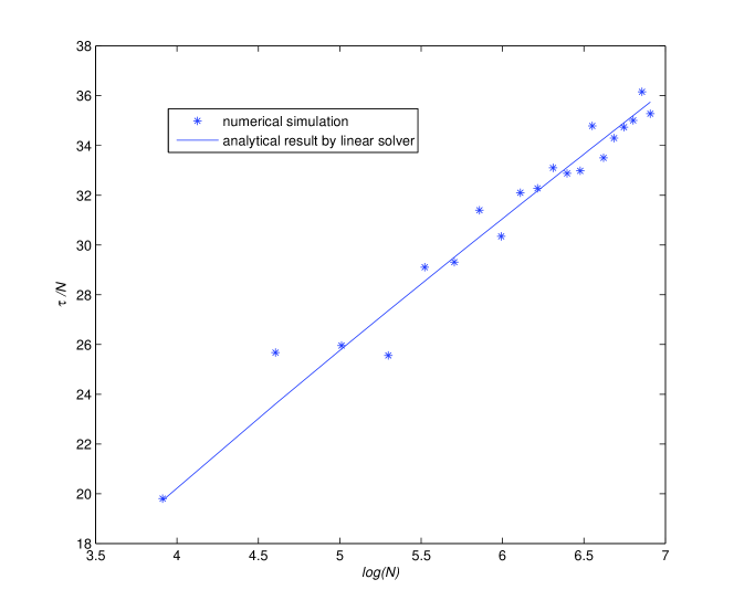
Figure 3: Consensus time (normalized by $N$) as a function of network size $N$ for 2-word naming game on complete graph. Each star point is an average of 10 runs of numerical simulations of 2-word naming game and the solid straight line consists of the solutions of the linear equation for each $N$.

Figure 4, depicting the expected number of time steps spent on each macrostate $T(n_{A},n_{B})$ when $N=100$ and $\vec{n}(0)=(50,50)$ shows that the time before absorption is mainly spent on the macrostates near the consensus states.

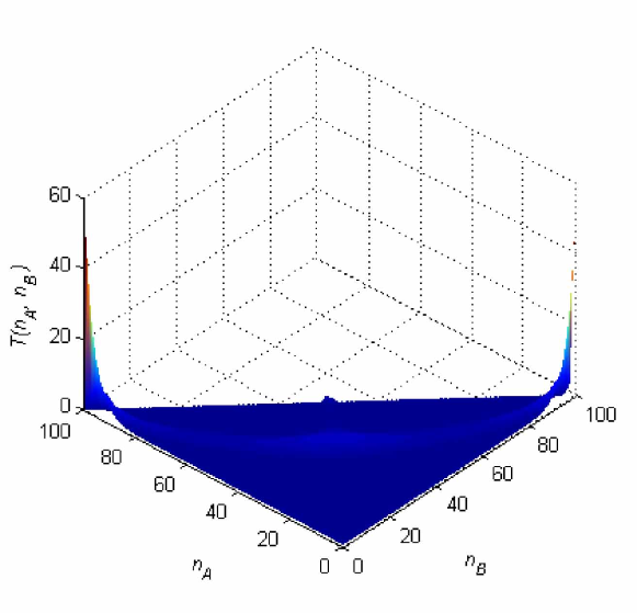
Figure 4: The expected time spent on each macrostate before consensus in the 2-word NG on a complete graph with $N=100$ nodes. The vertical axis $T(n_{A},n_{B})$ is the expected time that the random walk spends in macrostate $(n_{A},n_{B})$ before consensus, starting from the $(n_{A}(0),n_{B}(0))=(50,50)$ initial macrostate.

IV The 2-word naming game with external influence

The previous section focused on the time taken by the system to spontaneously reach consensus. A natural question that arises is how consensus can be sped up through an external influencing force such as mass media Mazitello_IJMP2007 ; Candia_JSTAT2008 , In this section we study this case: the 2-word NG subject to an external field of magnitude $f$ for which the update rule is defined as follows: in each time step, if the listener is in a mixed state i.e. AB, it will with probability $f$ spontaneously change into state A and with probability $1-f$ follow the original NG rule (Sec. III). All the differences between this case and the spontaneous case lie in the $\Delta\vec{n}(\vec{n})$ which are listed in Table 3.

Table 3: Update events for the 2-word naming game with central influence and the associated random walk transition probabilities

speaker	listener	event	$\Delta\vec{n}(n_{A},n_{B})$	probabilty
B or AB	A	$A\rightarrow AB$	(-1,0)	$P(A-)=n_{A}(N-n_{A}+n_{B})/2N^{2}$
A, AB or f	AB	$AB\rightarrow A$	(1,0)	$P(A+)=(1-f)(N-n_{A}-n_{B})(N+n_{A}-n_{B})/2N^{2}+f(N-n_{A}-n_{B})/N$
A or AB	B	$B\rightarrow AB$	(0,-1)	$P(B-)=n_{B}(N+n_{A}-n_{B})/2N^{2}$
B or AB	AB	$AB\rightarrow B$	(0,1)	$P(B+)=(1-f)(N-n_{A}-n_{B})(N-n_{A}+n_{B})/2N^{2}$
A, B or AB	A or B	unchanged	(0,0)	$P_{0}=(n_{A}+n_{B})/2N+(n_{A}-n_{B})^{2}/2N^{2}$

In Fig. 5 we show how the vector field $E[\Delta n]$ which is intuitively the “drift” part of the course-graining random walk changes at different influence levels $f$’s.

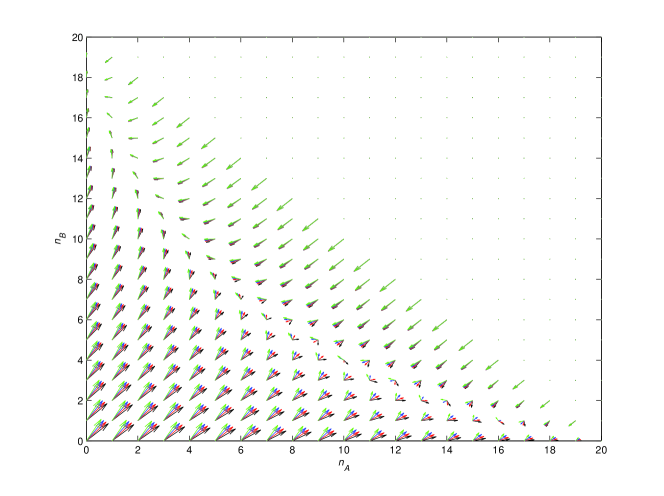
Figure 5: Several vector fields are drawn in this figure with different colors, each color show the drift of coarse-grained random walk $E[\Delta\vec{n}(\vec{n})]$ on a complete graph with $N=20$ nodes at different central influence levels $f$. The length of each vector has been rescaled to its square root to avoid cluttering the whole graph.

Following the first-step analysis, we can solve for the expected consensus time $\tau$ and the expected number of time steps spent at each macrostate $T(n_{A},n_{B})$ starting from any given macrostate. A specific solution of $T(n_{A},n_{B})$ on a complete graph with $N=100$ starting from macrostate $(50,50)$ is shown in Fig. 6. As shown, there are two peaks around the two consensus states, just as in the spontaneous case, although the peak near the consensus state which the external influence prefers (all A state) is much higher than the other one, even at a low influence level $f=0.05$.

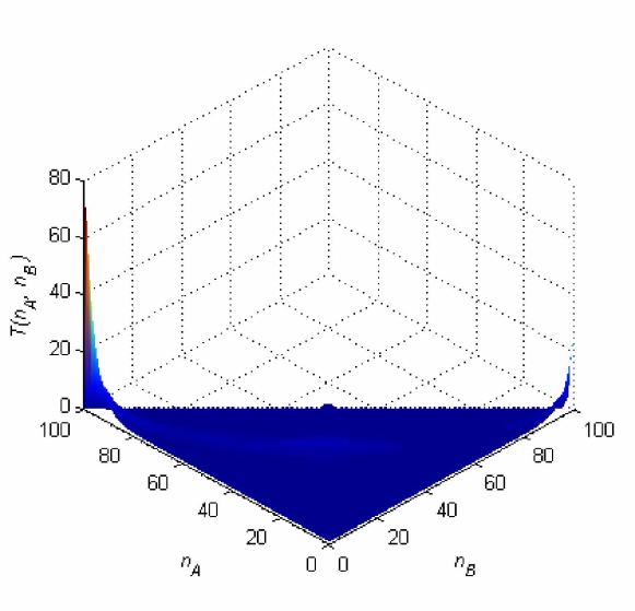
Figure 6: Expected time spent on each macrostate before consensus $T(n_{A},n_{B})$ in the 2-word NG on complete graph with $N=100$ with central influence $f=0.05$, starting from a unbiased initial macrostate $(n_{A}(0),n_{B}(0))=(50,50)$.

IV.1 First-step analysis of probability of consensus

To better understand the effect of external influence, we apply the first-step analysis on the probability of reaching a specific consensus state. Defining $P_{A}(\vec{n})$ as the probability of going to an all-$A$ consensus starting from the macrostate $\vec{n}=(n_{A},n_{B})$, $P_{A}(\vec{n})$ follows:

$$P_{A}(\vec{n}(t))=E[\mbox{$P_{A}(\vec{n}(t+1))$}]={\sum_{i\in\{(1,0),(-1,0),(0,1),(0,-1),(0,0)\}}P(\Delta\vec{n}(\vec{n})=i)\ P_{A}(\vec{n}+i)}$$ (11)

and satisfies the boundary conditions $P_{A}(N,0)=1$ and $P_{A}(0,N)=0$. Ordering $P_{A}(\vec{n})$ of all macrostates (including the two consensus states) in a vector $\vec{P_{A}}$, we rewrite the equations as $\vec{P_{A}}=Q_{0}\vec{P_{A}}$. $Q_{0}$ is a square matrix of order $(N+2)(N+1)/2$ and all its elements are given in Table III.

In Fig. 7, we consider the NG on 100-node complete graph starting from the macrostate $(n_{0},N-n_{0})$. For $n_{0}=50$ and central influence $f=0$ (the left end of the black curve), it has equal probability of going to all A and all B consensus. When $n_{0}<50$, it is more probable to go to all B consensus without central influence. However, with a biased central influence $f$, one can always convert the preference of the process to the opposite side - all A consensus.

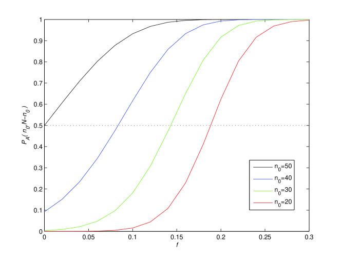
Figure 7: Probability of all A consensus $P_{A}$ with different external influence level $f$’s starting from macrostate $(n_{A},n_{B})=(n_{0},N-n_{0})$ on 100-node complete graph.

Furthermore, we show in Fig. 8 that the external influence becomes more powerful in forcing the network to a desired consensus state when network size $N$ grows larger. Starting from an unbiased macrostate $(N/2,N/2)$, the probability of going to all B consensus $1-P_{A}(N/2,N/2)$ (which is against of the central influence) decays exponentially along with the network size $N$. So it is reasonable to expect that in real social network for which network size $N$ is very large, a very slight biased central influence can strongly affect the social consensus.

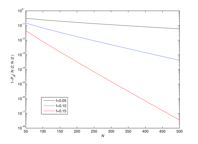
Figure 8: Probability of all B consensus $1-P_{A}$ starting from macrostate $(n_{A},n_{B})=(N/2,N/2)$ as a function of network size $N$ with different external influence level $f$’s.

V 2-word Naming Game with committed agents

A second method of speeding up consensus is by introducing an intrinsic bias in the system, through a set of inflexible agents Galam_PhysA2007 ; Lucomm promoting a designated opinion. We refer to such individuals as committed agents Lucomm . Intuitively, the introduction of committed agents will break the symmetry of the original NG and will facilitate global consensus to the state adopted by the committed agents. In this section we provide asymptotic solutions of 2-word NG with committed agents

Suppose that the number of committed agents is $n_{q}$ and all committed agents are in state $A$. The corresponding events in the NG with committed agents and the associated RW transition probabilities are summarized in Table 4.

Table 4: Update events for the 2-word naming game with committed agents and the associated random walk transition probabilities

speaker	listener	event	$\Delta\vec{n}(n_{A},n_{B})$	probabilty
B or AB	A	$A\rightarrow AB$	(-1,0)	$P(A-)=(n_{A}-n_{q})(N-n_{A}+n_{B})/2N^{2}$
A or AB	AB	$AB\rightarrow A$	(1,0)	$P(A+)=(N-n_{A}-n_{B})(N+n_{A}-n_{B})/2N^{2}$
A or AB	B	$B\rightarrow AB$	(0,-1)	$P(B-)=n_{B}(N+n_{A}-n_{B})/2N^{2}$
B or AB	AB	$AB\rightarrow B$	(0,1)	$P(B+)=(N-n_{A}-n_{B})(N-n_{A}+n_{B})/2N^{2}$
A, B or AB	A or B	unchanged	(0,0)	$P_{0}=(n_{A}+n_{B})/2N+(n_{A}-n_{B})^{2}/2N^{2}+n_{q}(N-n_{A}+n_{B})/2N^{2}$

The equations $\vec{\tau}=Q\vec{\tau}+\vec{t}$ and $(I-Q)^{T}u=\delta_{N}^{\vec{n}}$ are derived in exactly the same way as in the non-committed case.

From the dynamics of infinite systems with homogeneous mixing, one can expect Galam_PhysA2007 ; Xie_2011 , that there exists a critical value $q_{c}$ of the committed fraction $q=n_{q}/N$, above which consensus times drop dramatically. More specifically, for $q<q_{c}$ the phase space exhibits three fixed points: a “meta-stable” one, dominated by individuals in state B, an stable absorbing fixed point with all individuals in state A, and a “saddle” point separating them. Initializing the system in a configuration corresponding to macrostate $(n_{A}(0),n_{B}(0))=(n_{q},N-n_{q})$ (a small number of committed agents embedded among Bs), the system quickly relaxes to the meta-stable fixed point and stays there for times exponentially large with the system size (i.e., forever in an infinite system). As $q$$\to$$q_{c}$, the meta-stable fixed point and the saddle point merge, and become an unstable fixed point. For $q>q_{c}$, regardless of the initial configuration, the system quickly relaxes to the all-A absorbing fixed point. Figure 9 confirms the above scenario. Figure 9(a) and (b) show the consensus times as a function of the initial macrostate $(n_{A},n_{B})$ for $q<q_{c}$ and $q>q_{c}$, respectively. In the former case, $q<q_{c}$, the expected consensus time $\tau(n_{A},n_{B})$ is given by the equation $\vec{\tau}=Q\vec{\tau}+\vec{t}$. A fast drop-off in consensus time as a function of the initial configuration, observed for $q<q_{c}$ [Fig. 9(a)], indicates the presence of the saddle point. For $q>q_{c}$, there is only one stable fixed point (the absorbing one), so the consensus time starting from any initial configuration is short, including initial configurations in the vicinity of the previously meta-stable states [Fig. 9(b)].

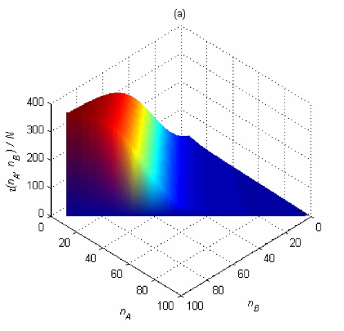
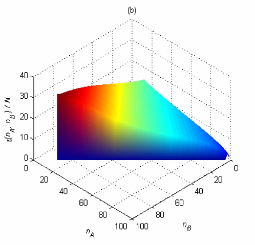
Figure 9: Expected normalized consensus time ($\tau(\vec{n})/N$) as a function of the initial macrostate $(n_{A},n_{B})$ on the complete graph with $N=100$ nodes. (a) when the fraction of committed agents is $q=0.06<q_{c}$; (b) when $q=0.12>q_{c}$.

Figure 10(a) and (b) present the expected number of time steps spent before absorption in each macrostate $T(n_{A},n_{B})$ starting from the initial state $(n_{q},N-n_{q})$ for $q<q_{c}$ and $q>q_{c}$, respectively. From Fig. 10(a) and (b), according to the two peaks in each figure, the random walk before absorption spend time mainly in two areas: one is near the meta-stable state [close to the initial state $(n_{q},N-n_{q})$], the other one is around the consensus state $(N,0)$. When $q<q_{c}$, the peak around the meta-stable state is dominant in the total consensus time, while for $q>q_{c}$, it can be ignored compared to the peak around consensus.

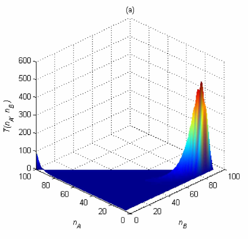
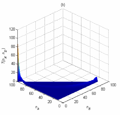
Figure 10: Expected time spent in each macrostate before consensus $T(n_{A},n_{B})$ on the complete graph with $N=100$ nodes, starting from the $(n_{A}(0),n_{B}(0))=(n_{q},N-n_{q})$ initial macrostate, (a) for $q=0.06<q_{c}$; (b) for $q=0.12>q_{c}$.

We sum $T(n_{A},n_{B})$ over these two areas separately (since the peak in Fig. 10 is very concentrated, the domain of summation does not matter very much), and define the time spent near consensus state as $T_{c}=\sum_{n_{A}>n_{B}}T(n_{A},n_{B})$ and that near the meta-stable state as $T_{m}=\sum_{n_{A}>n_{B}}T(n_{A},n_{B})$. Figure 11 shows that the normalized time spent near consensus $T_{c}/N$ has the same order $O(\ln(N))$ when $N$ grows as demonstrated in the non-committed case. We conclude that for different $q$’s regardless whether it is less or greater than the critical $q_{c}$, the peaks around the consensus state have roughly the same scale and are about twice the height of the corresponding peak in the 2-word NG without committed agents shown in Fig. 4. Figure 12 shows that the normalized time that the random walk is stuck in the vicinity of the meta-stable state, $T_{m}/N$, grows exponentially with $N$ for $q<q_{c}$, while it decreases weakly with $N$ for $q>q_{c}$. The crossover and departure from these drastically different scaling behaviors appears at around $q=0.08$, hence our rough estimate for the critical fraction of committed agents is $q_{c}\approx 0.08\pm 0.01$. A detailed finite-size analysis of this crossover behavior should be performed to extract $q_{c}$ in the infinite system-size limit. Since for the consensus time we approximately have $\tau\approx T_{m}+T_{c}$, the above findings imply that $\tau/N\sim O(e^{cN})$ (where $c$ is a constant) for $q<q_{c}$, while $\tau/N\sim O(\ln(N))$ for $q>q_{c}$.

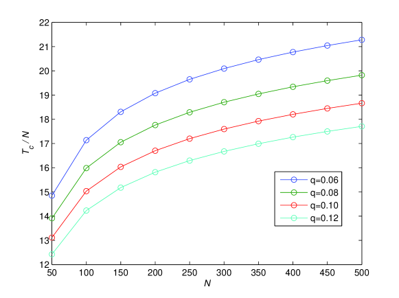
Figure 11: Normalized time spent near the consensus state before consensus as a function of network size $N$ for different fraction of committed agents $q$, including cases for both $q<q_{c}$ and $q>q_{c}$.

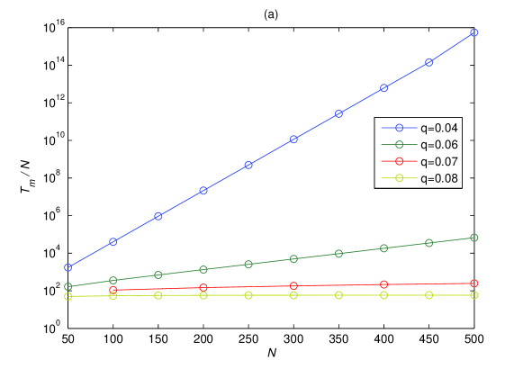
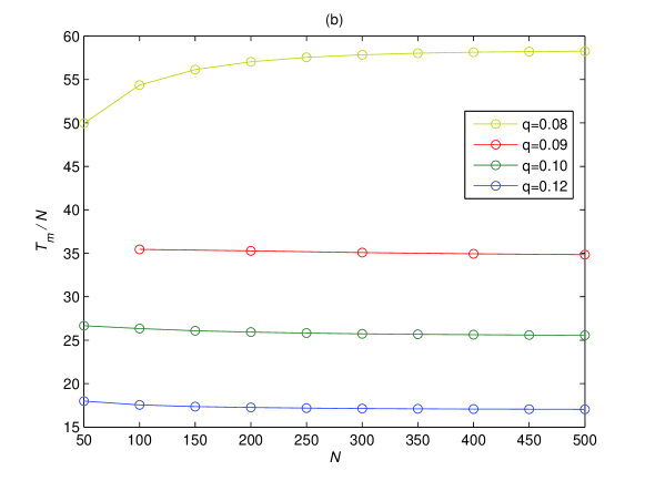
Figure 12: Normalized time spent near the meta-stable state as a function of network size $N$ for different fraction of committed agents $q$, (a) for $q<q_{c}$; (b) for $q>q_{c}$. The behavior for $q=0.08$ is shown in both (a) and (b), corresponding to our rough estimate of the critical fraction of committed agents, $q_{c}\approx 0.08\pm 0.01$.

VI Summary

We studied influencing and consensus formation, in particular, the asymptotic consensus times, in stylized individual-based models for social dynamics on the complete graph. We accomplished this by a coarse-graining approach (lumping microscopic variables into macrostates) resulting in an associated random walk. We then analyzed first-passage times (corresponding to consensus) and times spent in each macro-state of the random-walk model. The method yields asymptotically exact consensus times for large but finite complete graphs of size $N$. Direct individual-based simulations can become time consuming for large systems and prohibitive even for moderately-sized systems when the system initially is in a meta-stable configuration, as the escape time can increase exponentially with the system size. The method presented here provides an alternative way to obtain the asymptotic behavior of consensus times, including the cases associated with extremely slow meta-stable escapes.

After testing this framework on spontaneous opinion formation in two known models, we applied it to two scenarios for social influencing in a variation of the 2-word naming game. First, we considered the case when individuals are exposed to a global external field (or central influence). We found that the external field dominates the consensus in the large network-size limit. Second, we investigated the impact of committed individuals with a fixed designated opinion (i.e., individuals who can influence others but themselves are immune to influence). In the latter case, we found the existence of a tipping point, associated with the disappearance of the meta-stable state in the opinion space: When the fraction of committed nodes is below a critical value, consensus times increase exponentially with system size; on the other hand when the fraction of committed nodes is above this threshold value (tipping point) the system is quickly driven to consensus with weak system size dependence.

While the method and the results presented here are applicable to the complete graph, consensus times often exhibit the same asymptotic scaling with the system size in large homogeneous sparse random networks Castelano_PRE2005 ; DallAsta_PRE2006 ; Lu_PRE2008 , hence our results yield some insight how ordering and consensus can evolve in realistic social networks. In particular, one can better understand and predict timescales associated with reaching consensus in social networks.

References

- (1) C. Castellano, S. Fortunato, V. Loreto, Rev. Mod. Phys. 81, 591 (2009).
- (2) S. Galam, Int. J. Mod. Phys. C 19, 409 (2008).
- (3) X. Pan and J. Yang, in Complex Systems and Complexity Science vol. 6, no. 2, pp. 87–92 (2009).
- (4) P.L. Krapivsky, Phys. Rev. A 45, 1067 (1992).
- (5) L. Frachebourg and P.L. Krapivsky, Phys. Rev. E 53, R3009 (1996).
- (6) E. Ben-Naim, L. Frachebourg, and P.L. Krapivsky, Phys. Rev. E 53, 3078 (1996).
- (7) I. Dornic, H. Chaté, J. Chave, and H. Hinrichsen, Phys. Rev. Lett. 87, 045701 (2001).
- (8) A. Baronchelli, M. Felici, E. Caglioti, V. Loreto and L. Steels, J. Stat. Mech.: Theory Exp. P06014 (2006).
- (9) Q. Lu, G. Korniss, and B.K. Szymanski, Phys. Rev. E 77, 016111 (2008).
- (10) Q. Lu, G. Korniss ,B.K. Szymanski, J. Econ. Interact. Coord. 4, 221 (2009) .
- (11) C. Castellano, V. Loreto, A. Barrat, F. Cecconi, and D. Parisi, Phys. Rev. E 71, 066107 (2005).
- (12) L. Dall’Asta, A. Baronchelli, A. Barrat, and V. Loreto, Phys. Rev. E 74, 036105 (2006).
- (13) L. Steels, Artificial Life 2, 319 (1995).
- (14) L. Dall’Asta and A. Baronchelli, J. Phys. A: Math. Gen. 39, 14851 (2006).
- (15) A. Baronchelli, L. Dall’Asta, A. Barrat and V. Loreto, Phys. Rev. E 73, 015102 (2006).
- (16) A. Baronchelli, V. Loreto, L. Steels, Int. J. Mod. Phys. C 19, 785 (2008).
- (17) L. Dall’Ast and T. Galla, J. Phys. A:Math. Gen 41, 435003 (2008)
- (18) F. Vazquez, X. Castelló and M. San Miguel J. Stat. Mech. Theory. Exp. P04007 (2010)
- (19) F. Slanina and H. Lavicka, Eur. Phys. J. B 35, 279 (2003).
- (20) V. Sood, T. Antal, and S. Redner, Phys. Rev. E 77, 041121 (2008).
- (21) X. Castelló A. Baronchelli, and V. Loreto, Eur. Phys. J. B 71, 557 (2009).
- (22) T.M. Liggett, Interacting Particle Systems (Springer-Verlag, New York, 1985).
- (23) P. Bremaud, in Markov chains: Gibbs fields, Monte Carlo simulation, and queues (Springer, 1991), pp. 253–311.
- (24) K.I. Mazzitello, J. Candia, and V. Dossetti, Int. J. Mod. Phys. 18 1475 (2007).
- (25) J. Candia and K.I. Mazzitello, J. Stat. Mech. Theory. Exp. P07007 (2008).
- (26) S. Galam, Physica A 381 366, (2007).
- (27) J. Xie, S. Sreenivasan, G. Korniss, W. Zhang, and C. Lim, B.K. Szymanski, preprint (2011).