Tropical Cyclones as a Critical Phenomenon

Abstract

It has been proposed that the number of tropical cyclones as a function of the energy they release is a decreasing power-law function, up to a characteristic energy cutoff determined by the spatial size of the ocean basin in which the storm occurs. This means that no characteristic scale exists for the energy of tropical cyclones, except for the finite-size effects induced by the boundaries of the basins. This has important implications for the physics of tropical cyclones. We discuss up to what point tropical cyclones are related to critical phenomena (in the same way as earthquakes, rainfall, etc.), providing a consistent picture of the energy balance in the system. Moreover, this perspective allows one to visualize more clearly the effects of global warming on tropical-cyclone occurrence.

Keywords power laws, scaling, self-organized criticality, power dissipation index, hurricanes

1 Introduction

A fundamental way to characterize a physical phenomenon is by analyzing the fluctuations of the energy it releases over successive occurrences. Of course, in most of the cases this is not a simple issue. For tropical cyclones, Bister and Emanuel Bister_Emanuel have found that the dissipated energy $E$ can be estimated by integrating the cube of the surface velocity field over space and time, by means of the formula

$$E\simeq\int\rho C_{D}|v(\vec{r},t)|^{3}d^{2}r\,dt,$$ (1)

with $\rho$ the surface air density, $C_{D}$ the surface drag coefficient, and $v(\vec{r},t)$ the surface wind speed at position $\vec{r}$ and time $t$. It is implicit in the formula that the main contribution to dissipation comes from the atmospheric surface layer.

In order to obtain the distribution of energy then, one only needs to apply the previous formula to as many tropical cyclones as possible (without any selection bias) and perform the corresponding statistics. However, in practice, the available records do not allow such a detailed calculation: instead of providing a nearly instantaneous velocity field, best-track data consist of a single value of the speed reported every six hours (the maximum sustained surface wind speed).

Emanuel has envisaged a way to reconcile the calculation of the energy with the limitation of the data Emanuel_nature05 . First, $\rho$ and $C_{D}$ can be approximated as constants in Eq. (1). Second, one can apply the similarity between radial profiles of speeds for different tropical cyclones to write $v(\vec{r},t)=v_{m}(t)f(\vec{r}/R(t))$, where $R(t)$ is the radius of storm at time $t$ (no matter how it is defined), $v_{m}(t)$ is the maximum of the surface velocity field for all $\vec{r}$ at $t$, and $f$ is the function that describes the shape of the velocity profile (the same for all storms, the scale given by $v_{m}$ and $R$). This yields a scaling between the integral over space on the one side and the maximum speed and the radius on the other (with the same constant of proportionality), and then,

$$E\propto\int|v_{m}(t)|^{3}R^{2}(t)dt,$$

where the symbol $\propto$ indicates proportionality. An additional approximation is that the radius of the storm is nearly uncorrelated with the speed, and therefore assigning a common radius to all storms (al all times) leads only to random errors in the evaluation of the energy. Finally, enlarging the integration time step up to $\Delta t=$ 6 hours gives

$$E\propto PDI\equiv\sum_{t}v_{t}^{3}\Delta t,$$

with $PDI$ defining the so-called power dissipation index, which is then a proxy for the total energy dissipated by a tropical cyclone during all its life. The symbol $v_{t}$ denotes the maximum sustained surface wind speed.

A similar definition is that of the so-called accumulated cyclone energy ($ACE$) Bell ; Gray_HDP , which integrates kinetic energy over time,

$$ACE\equiv\sum_{t}v_{t}^{2}\Delta t,$$

where the essential difference with the $PDI$ is the replacement of the cube of the speed by a square. Note that the time integral of the kinetic energy is not an energy, unless some proportionality factors are introduced in the formula, in the same way as in Eq. (1). In any case, in this work we will study the distribution of energy dissipated by tropical cyclones using both $PDI$ and $ACE$ as proxies for the energy, evaluated over the complete lifetime of the storms.

2 Power-Law Distribution of the Energy of Tropical Cyclones

In order to describe probability distributions we will use the probability density function. For the case of power dissipation index this is defined as the probability that the value of this variable lies in a narrow interval of size $dPDI$ around a concrete $PDI$, divided by $dPDI$ to make the result independent on $dPDI$, i.e.,

$$D(PDI)\equiv\frac{\mbox{Prob[ $PDI-dPDI/2\leq$ value $<PDI+dPDI/2$ ]}}{dPDI},$$

where Prob denotes probability, which is evaluated as the number of events that fulfill the condition divided by the total number of events. This definition ensures normalization, $\int_{0}^{\infty}D(PDI)dPDI=1$. Note also that the units of the density are the reciprocal of the units of the variable, so, for $D(PDI)$ these are s${}^{2}/$m³ (if the $PDI$ is measured in m³/s²). An analogous definition applies to the probability density of the $ACE$, $D(ACE)$, or of any other variable.

Recently, we have shown that the distribution of $PDI$ in different tropical-cyclone basins follows a power law,

$$D(PDI)\propto 1/PDI^{\alpha},$$

except for the largest and smallest values of $PDI$. The exponent $\alpha$ turns out to be close to 1 (between 1 and 1.2, roughly) Corral_hurricanes . Note that an exponent equal to one implies that all decades contribute in the same proportion to the total number of events, in other words, any interval of $PDI$ values in which the extremes keep the same proportion contains the same probability.

The calculation of $D(PDI)$ is not direct, though. The quantity of interest, the $PDI$, varies across a broad range in the basins studied, from less than $10^{9}$ m³/s² to more that $10^{11}$ m³/s², being necessary to plot the distribution in logarithmic axes in order to represent the different scales. Moreover, this has the advantage that on a log-log plot a power law appears as a straight line (note that this is not the case for the cumulative distribution function if the power law has an upper cutoff Hergarten_book ).

On the other hand, the broad range of variation also makes inappropriate the use of a constant interval size $dPDI$ (essentially, $dPDI$ should be large enough to contain enough statistics but small enough to provide a complete sampling of the range of variation of $D(PDI)$). Logarithmic binning is a solution to this problem Hergarten_book , where the size of the bins appears as constant in the logarithmic scale used. (An equivalent, simpler solution, is to work with the distribution of $\ell\equiv\ln PDI$, calculating its probability density $D(\ell)$ using standard linear binning and then obtaining the $PDI$ density by means of the change of variable $D(PDI)=D(\ell)d\ell/dPDI=D(\ell)/PDI$; of course, $D(PDI)$ and $D(\ell)$ have different functional forms, despite the ambiguous notation.) Naturally, similar considerations hold for the distribution of $ACE$.

Turning back to the results of Ref. Corral_hurricanes , it is shown there that the $PDI$ distribution is well described by a decreasing power law in the North Atlantic (NAtl), the Northeastern and Northwestern Pacific (EPac and WPac), and the Southern Hemisphere (SHem) basins, with an exponent $\alpha$ ranging from $0.98\pm 0.03$ in the WPac to $1.19\pm 0.07$ in the NAtl, where the uncertainty refers to one standard deviation of the maximum-likelihood-estimator mean value. The power law holds from a range of a bit more than one decade (for the NAtl and the EPac) up to two decades (for the WPac). The data used were the best tracks from NOAA’s National Hurricane Center for NAtl and EPac NOAA ; NOAA_hurdat and from US Navy’s Joint Typhoon Warning Center for WPac and SHem ATCR_report ; JTWC_data . Here we will use the same data sets.

[scale=.55]fig1a.ps

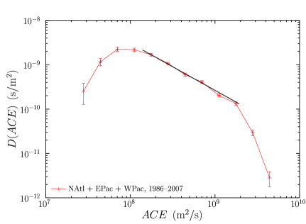
Figure 1: Probability density of tropical-cyclone dissipated energy, for the NAtl, EPac, and WPac basins, during 1986–2007, compressing 1212 storms. (a) $PDI$ probability density, $D(PDI)$, together with the number of tropical cyclones in each bin per year $n(PDI)$. A maximum-likelihood fit of the distribution between the values $3.2\cdot 10^{9}$ and $4.0\cdot 10^{10}$ m${}^{3}/$s² yields $\alpha=1.07\pm 0.06$ with a $p-$value $=99\pm 0.3\%$ (calculated generalizing the method of Ref. Clauset , with a resolution in the optimization of 10 points per decade). (b) $ACE$ probability density. A maximum-likelihood fit between the values $1.6\cdot 10^{8}$ and $2.0\cdot 10^{9}$ m${}^{2}/$s. yields $\alpha=1.10\pm 0.05$ with a $p-$value $=59\pm 1.6\%$.

As an illustration, we show in Fig. 1(a) the $PDI$ distribution for the Northern Hemisphere (excluding the Indian Ocean, i.e., only NAtl+EPac+WPac) for the years 1986 to 2007. Tropical depressions (storms whose maximum sustained surface wind speed does not exceed 34 knots), not included in the NAtl and EPac records, have been eliminated from our analysis of the WPac, for consistency. Of course, the results are in agreement with Ref. Corral_hurricanes , with an exponent $\alpha=1.07\pm 0.06$.

If instead of the $PDI$ we use the $ACE$ the results do not change in essence, yielding $\alpha=1.10\pm 0.05$, as displayed in Fig. 1(b). The reason for the coincidence of results between both variables is due to the fact that they are highly (though non-linearly) correlated. Figure 2 shows a scatter plot for the values of the $PDI$ versus the $ACE$, using the same data as above. A linear regresion applied to $\ln PDI$ versus $\ln ACE$ yields $PDI\propto ACE^{\gamma}$, with $\gamma\simeq 1.36$ and a correlation coefficient $\varrho=0.994$. If we write our probability distributions as $D(PDI)\propto 1/PDI^{1+\beta_{p}}$ and $D(ACE)\propto 1/ACE^{1+\beta_{a}}$, and introduce $PDI\propto ACE^{\gamma}$ in the identity relation $D(PDI)=D(ACE)dACE/dPDI$, one gets $\beta_{a}=\gamma\beta_{p}$, which implies that a power law with exponent $\alpha=1$ (i.e., $\beta=0$) is invariant under power-law changes of variables. These results are in good concordance with our numerical findings.

[scale=.55]fig_scatter.ps

Figure 2: Non-linear correlation between $PDI$ and $ACE$. The former variable is plotted versus the latter for all hurricanes, typhoons, and tropical storms occurring in the NAtl, EPac, and WPac for the period 1986–2007. A power-law correlation $PDI\propto ACE^{1.36}$ shows up, with a corresponding linear correlation coefficient (for the logarithm of the variables) $\rho=0.994$. The two regression lines are included, although they overlap.

[scale=.65]map0.ps

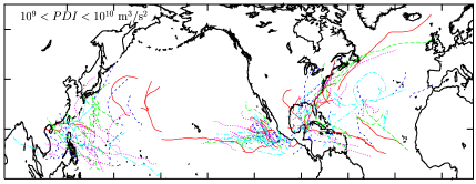
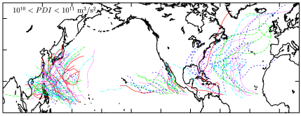
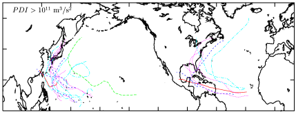
Figure 3: Trajectories of hurricanes, typhoons, and tropical storms (i.e., excluding tropical depressions) in the WPac, EPac, and NAtl, separated for different values of the $PDI$. Different line styles correspond to different years, from 2003 to 2007. The top panel points to the incompleteness of the record for the smallest $PDI$ values, whereas the bottom panel shows that the tropical cyclones with the largest $PDI$ values tend to travel through the whole basin.

An important issue is the deviation of the distribution from the power-law behavior for small and large energies. In the first case, the deviation is due to the scarcity of data referring to small storms. The best tracks of the National Hurricane Center (for NAtl and EPac) do not contain tropical depressions, so the data are truncated including only hurricanes (of category 1 at least) and tropical storms (maximum sustained surface wind speed larger than 34 knots but below hurricane category). In the case of the best tracks of the Joint Typhoon Warning Center some tropical depressions are included, but these are very few, only those ones which are consider “significant”. This artificial truncation of the data obviously makes the distribution depart from the power-law behavior for small values of the energy. The paths of the tropical cyclones of a small part of the record, just for the 5 year period 2003-2007, are shown in Fig. 3, separated in distinct $PDI$ ranges; the top panel shows how the set of storms with $PDI<10^{9}$ m${}^{3}/$s² seems certainly incomplete.

More fundamental is a decay faster than power law for large values of the energy. We suggest in Ref. Corral_hurricanes that this is due to a finite size effect: the spatial size of the basin is not big enough to sustain tropical cyclones with larger $PDI$ values (remember that the $PDI$ integrates $v_{t}^{3}$ over time, and time can be considered equivalent to space). Indeed, when a tropical cyclone in any of the basins considered reaches a $PDI$ of about $10^{11}$ m³/$s^{2}$ it is very likely that its evolution is affected by the boundaries of the basin, which are constituted essentially either by continental land or by a colder environment; this deprives the tropical cyclone from its source of energy in the form of warm water and provokes its attenuation and eventual death, see Fig. 3(d). Under the name “colder environment” we can compress both a low sea surface temperature (as it happens in high latitudes or with the cold California Current) or the presence of extratropical weather systems. In any case, this makes the boundaries of the basin be not fully “rigid” in contrast to condensed matter physics (even for the case of continental boundaries, there have been hurricanes that have jumped from the NAtl to the EPac).

Another relevant issue to take into account is up to what point the power law is the right distribution to fit the $PDI$ and $ACE$ distributions. We have shown in Ref. Corral_hurricanes that the power law provides indeed a good fit, but this does not exclude that other distributions can fit the data equally well, or even better. In fact, any power law in a finite domain (let us say, with the variable $x$ in between $m_{1}$ and $m_{2}$) can be fit also by a lognormal distribution, with a $\sigma$-parameter (the standard deviation of the underlying normal distribution) which tends to infinity. Indeed, the lognormal probability density,

$$D(x)\propto\frac{1}{x}\exp\left(-\frac{(\ln x-\mu)^{2}}{2\sigma^{2}}\right),$$

can be written as

$$D(x)\propto\frac{1}{e^{\mu}}\left(\frac{e^{\mu}}{x}\right)^{1+(\ln x-\mu)/(2\sigma^{2})}.$$

This is a kind of pseudo-power-law, with a pseudo-exponent $1+(\ln x-\mu)/\sigma^{2}$ that changes very slowly with $x$ if $\sigma$ is big enough. Taking $m_{1}\equiv e^{\mu+\sigma^{2}\epsilon_{1}}$ and $m_{2}\equiv e^{\mu+\sigma^{2}\epsilon_{2}}$, the pseudo-exponent changes from $1+\epsilon_{1}$ for $x=m_{1}$ to $1+\epsilon_{2}$ for $x=m_{2}$, and the extreme values $m_{1}$ and $m_{2}$ can be as large as desired if $\sigma$ is big enough. Note, anyhow, that the lognormal distribution has two parameters ($\mu$ and $\sigma$), whereas the power law has just one ($\alpha$). A similar argument can be presented for other long-tailed distributions. In conclusion, the choice of the right fit is a problem that cannot be solved only by means of the statistical analysis, and it is the physical knowledge which has to provide a criterion to select the most appropriate distribution. The rest of this work will justify the preferability of the power law as a physical model of tropical-cyclone dissipation distribution.

3 Power-Law Distribution of Earthquake Energies

The power-law distribution of energy dissipation in tropical cyclones is analogous to the well known Gutenberg-Richter law of earthquakes. Let us see how. This law states that, for a given spatial region and over a certain period of time, the number of earthquakes with magnitude larger than $M$ is about 10 times greater than the number of earthquakes with magnitude larger than $M+1$, which in its turn is 10 times greater than the number of earthquakes larger than $M+2$ and so on Kanamori_rpp . In mathematical terms, the number of earthquakes above $M$, denoted by $N(M)$, is a decreasing exponential function,

$$N(M)\propto 10^{-bM}$$

where the $b-$value is a parameter close to 1.

The cumulative distribution function of magnitudes, defined as $S(M)\equiv$ Prob[ magnitude value $\geq M$ ] is estimated directly from $N(M)$ as $S(M)=N(M)/\mathcal{N}$, where $\mathcal{N}$ is the total number of earthquakes considered, of any magnitude. It is obvious that the cumulative distribution is exponential, and therefore the density, given as $D(M)=-dS(M)/dM$, is an exponential too, with the same $b-$value. (This allows that, when working with magnitude distributions, one does not need to specify if one is measuring the density or the cumulative distribution, unfortunately. Of course, this is only acceptable for exponential distributions).

But magnitude is not a physical variable (it has no units). It is believed, at least as a first approximation, that the energy $E$ radiated in an earthquake is an exponential function of the magnitude, $E\propto 10^{3M/2}$ (with a proportionality factor between $10^{3}$ and $10^{5}$ Joules) Kanamori_rpp . Therefore, the energy probability density will be a power law,

$$D(E)=D(M)dM/dE\propto D(M)/E\propto 1/E^{1+2b/3}.$$

Note that, as in the case of tropical cyclones, we have used the same symbol for the density of energies and for the density of the logarithm, although the functional form of each one is not the same (power law versus exponential, respectively).

Summarizing, although the Gutenberg-Richter law implies an exponential distribution of the magnitudes of earthquakes, in terms of the radiated energy the Gutenberg-Richter law is given by a power law. Then, the fundamental difference in the structure of energy release between earthquakes and tropical cyclones is only quantitative and not qualitative, as both phenomena follow power-law distributions of energy with $\alpha\simeq 1.7$ in the first case and $\alpha\simeq 1.1$ for tropical cyclones. Another difference is the deviation from the power-law behavior at the largest values of the energy in tropical cyclones; in the case of earthquakes the existence or not of this boundary effect is not clear Kagan_calcutta ; Main_ng .

In fact, many other complex phenomena in the geosciences yield power-law distributions of energies, or, broadly speaking, “sizes”. These phenomena include, in addition to earthquakes and tropical cyclones: rainfall Peters_prl , landslides and rock avalanches Malamud_hazards ; Frette96 , forest fires Malamud_science , volcanic eruptions Lahaie , solar flares Arcangelis ; Baiesi_flares , the activity of the magnetosphere Wanliss , tsunamis Burroughs , and perhaps meteorite impacts Chapman . Nevertheless, the power laws are not totally ubiquitous, see for instance Ref. Corral_fires .

4 Relevance and Mechanisms for Power-Law Distributions

Which are the implications of having a power-law distribution, as it happens for the released energy of tropical cyclones, earthquakes and other phenomena just mentioned? In general, power-law distributions denote the presence of three main characteristics:

• Divergence of the mean value of the variable.

• Absence of a characteristic scale.

• Possible connection with criticality.

Let us explain each one.

4.1 Divergence of the mean value

Regarding the first issue, it is obvious that, if we consider the mean energy value, this fulfills $\langle E\rangle\equiv\int_{m}^{\infty}ED(E)dE=\infty$, if the power law exponent $\alpha$ is smaller than 2 (but larger than 1 for normalization), with $m$ the minimum value of the energy. Note that this is a property which is neither a characteristic of all power laws nor exclusive of some power laws (there are many other distributions which show this divergence, for instance, $D(E)\propto E^{-\alpha}\cos^{2}E$).

Obviously, from a physical point of view, the mean energy dissipated by a phenomenon as earthquakes or hurricanes cannot be infinite (the Earth has a finite energy content) and therefore the power-law behavior cannot be extrapolated to infinity. But if we do not know up to which maximum energy value the power law holds (which seems to be the case of earthquakes, but not that of tropical cyclones), the mean value of the energy is not defined and its calculation from any data set does not converge. What happens is that the scarce extreme events dominate the calculation of the average, as when they occur their contribution to the mean value is large enough to alter significantly this mean value. So, the fluctuations are the most significant trend of the energy, and not the mean value. In the case of tropical cyclones, we can only say that if it were not for the finite-size effects imposed by the boundaries of the basins, the mean released energy could not be calculated.

4.2 Lack of characteristic scale

In contrast to the first one, the second property, the absence of any characteristic scale for the energy release, is an exclusive property of power laws Christensen_Moloney . It is possible to show that a power-law function $g(x)\propto 1/x^{\alpha}$ (with $-\infty<\alpha<\infty$) is the only solution to the scale-invariance condition: $g(x)=cg(x/a),\,\forall x,\forall a$, where it turns out then that $c$ has to be related to $a$ by $c=1/a^{\alpha}$ (alternatively, fixing the relation between $a$ and $c$ determines the value of the exponent $\alpha$). This condition means that it does not matter in which scale we look at the variable $x$, we will see the same shape for the function $g(x)$. For example, let us take $a=1000$, then, when we write $x/a$ we are looking at $x$ at a scale that is 3 orders of magnitude smaller than the original one (we go from the scale of kilo-Joules to Joules, let us say); if we take $c=0.01$, which means that we are performing another linear transformation in the $y-$axis, we find that the corresponding scale-invariant function is $g(x)\propto 1/\sqrt[3]{x^{2}}$, indeed, $\alpha=-\log c/\log a=2/3$. Another example is given in Fig. 4.

[scale=.55]fig4a.ps

Figure 4: Illustration of the scale invariance of power laws. A power-law function with $\alpha=-0.5$ looks exactly the same at two different scales. The box in the top panel is enlarged in the bottom one, the scale factors of the scale transformation are $a=4$ and $c=1/a^{\alpha}=2$.

Nevertheless, there is a “little” problem regarding scale invariance of probability distributions: a function of the kind $g(x)\propto 1/x^{\alpha}$ cannot be a probability density for all $x$, even for just $x>0$, as $\int_{0}^{\infty}g(x)dx=\infty$, for all $\alpha$. In practice, it is necessary a small-energy cutoff $m$ if $\alpha\geq 1$ or a large-energy cutoff if $\alpha\leq 1$, so, the scale invariance only can exist for a range of $x$ and $a$, and not for all of them.

4.3 Criticality

One has to recognize that scale invariance is a rather strange property. How can it be that the relative proportion of the value of a physical observable at two different values of its variable, $g(x)/g(x/a)$, is the same ($=c$) at the milli-scale and at the Mega-scale (i.e., independent on $x$) if the values $x$ and $x/a$ take a constant proportion ($a$)? This means that the study of the function $g$ does not allow us to distinguish the scale of observation (in order words, $g$ cannot be used as an $x-$meter). It seems obvious that the same physics has to operate at very different scales.

In order to elucidate how scale invariance in energy distributions is achieved we need a model of the energy release. Let us have in mind the case of earthquakes, just to fix ideas. There, energy is released in tectonic faults in an avalanche-like process. The picture can be summarized as follows: stress in the Earth crust displays very small changes; sooner or later, at some point in the crust, the static friction cannot sustain a small variation in stress and a slip takes place; this local slip increases the stress in the neighboring area, where more slip can be induced in this way, and so on.

A very simple model of this process is given by a chain of dominoes: the slip at a fault patch is represented by the toppling of one piece; a sequence of topplings, until the end of the activity, constitutes an avalanche that represents an earthquake (or other phenomenon); and the energy released in the process will be proportional to the number of topplings, which is called the avalanche size. In the usual game, the toppling of one piece induces the toppling of the next and so on; this is the so-called domino effect and yields toppling events (avalanches) whose size is equal to the size of the system (the number of topplings equals the total number pieces). We arrive then to the so-called characteristic-earthquake model. But this is not what the data tells us; the Gutenberg-Richter law shows that there should be avalanches of all sizes, with no characteristic scale.

We need to modify the domino model. Instead of having that one toppling always induces just one toppling, let us consider that one toppling induces one toppling, or none, or may be two, or three, etc. That is, we have a random number of topplings, with the probability of the number of induced topplings given by the same probability distribution for all pieces. For this purpose it is convenient to imagine not a one-dimensional domino chain but an array of pieces. Mathematically, this is just an image of a simple branching process, introduced in science to describe in the first place the growth and extinction of populations.

The outcome of a branching process depends on the so-called branching ratio $B$, which is the average number of topplings induced directly by a single toppling (from one time step to the next) Harris ; Sornette_critical_book . It is clear that if $B>1$ the process will have a tendency to grow exponentially, giving rise to a system-spanning avalanche (although there is also a finite probability that the chain of topplings dies spontaneously); in contrast, if $B<1$, the activity attenuates fast, on average, and the size of the avalanches is small. However, if $B$ is precisely equal to one (with a standard deviation different than zero) these two tendencies compensate, and then we loose any characteristic scale in the size of the avalanches: they are power-law distributed, the concrete shape of the density being $D(s)\propto 1/s^{3/2}$, with $s$ the size of the avalanche (proportional to the energy). This case is called a critical branching process.

So, in principle, we have arrived at a reasonable model to generate power-law distributions, just adjusting the branching ratio to be equal to one. The next question in order to give an explanation of these phenomena is of course how the fine tuning of the branching ratio is achieved in nature. An answer is given by the idea of self-organized criticality proposed by Bak et al. in the 80’s Bak_book ; Jensen . The basic idea is the existence of a feedback mechanism that keeps the branching ratio close to one; if it is larger than one this produces large avalanches and in this case the branching ratio is reduced (the distance between the domino pieces is increased somehow); if the branching ratio is small, the avalanches are small, and then the branching ratio is increased Zapperi_branching .

The idea is better illustrated substituting the toppling of domino pieces by the toppling of grains in a sandpile BTW87 ; Christensen_oslo . The advantage of the sandpile is that after a large avalanche (which usually happens for high $B$), many grains leave the pile through its open boundaries (the pile is built over a finite support) and this decreases the average slope of the pile, making more difficult the toppling of the remaining grains and reducing then the branching ratio. On the contrary, when small avalanches predominate (low $B$) the grains do not reach the boundaries of the pile, and a subsequent slow addition of more grains increases the slope and also the branching ratio (as the toppling of the grains is facilitated by a steeper pile).

The ideal sandpile is a particular realization of one kind of systems called slowly driven, interaction-dominated threshold systems Jensen , whose three main ingredients are, as the name denotes: a slow energy input, an intermediate energy storage caused by local thresholds, and sudden bursty energy releases that spread through the system Peters_JH . The energy input comes from the slow addition of grains and the energy storage is in the form of potential energy of the metastable configurations of the grains, which are possible thanks to the thresholds built by the static friction between grains. When the input of grains makes one of the thresholds to be overpassed, some grains start to move, this helps other grains to overpass their thresholds, giving rise (or not) to an energy release in the form of an avalanche.

Earthquakes also fulfill this picture. In this case the slow energy input comes from the relative motion of the tectonic plates, this energy is stored in the form of stress in the faults, due again to the thresholds provided by static friction. When an increase in stress cannot be sustained by friction, energy is released and redistributed in the system, triggering an avalanche of slips, i.e, an earthquake.

Among the geophysical phenomena mentioned at the end of Sec. 3 as displaying power-law statistics in their energy release, most of them (rainfall, landslides, rock avalanches, forest fires, volcanic eruptions, magnetosphere activity, and solar flares) can be understood as self-organized critical systems, see Table 4.3. Perhaps, the only exceptions are tsunamis, which are not slowly driven (but driven by earthquakes, landslides, etc.), and may be meteorites. In the next section we will discuss if the evolution of tropical cyclones can be understood in these terms.

Table 1: Self-organized critical characteristics of diverse phenomena. All systems receive a slow driving of energy which is stored thanks to local thresholds; eventually, a sudden release of energy spreads through the system.

	sandpile	earthquakes	rainfall	tropical cyclones
driving		addition	motion of	solar	solar
	of grains	tectonic plates	radiation	radiation
storage of	gravitational	elastic	water in	heat of the sea
energy	potential energy	potential energy	atmosphere
threshold	friction	friction	saturation	sea surface temperaturea
spread of	toppling of	release	nucleation	wind
energy	grains	of stress	of drops

^a Plus a external trigger.

5 Criticality of Tropical Cyclones

Previously we have shown that the energy dissipated by tropical cyclones follows a power-law distribution. As other catastrophic phenomena also show this behavior, and as some of these other complex phenomena can be accommodated to the perspective of self-organized criticality, it is natural to investigate the possible connections between self-organized criticality and tropical cyclones.

In principle, we can guarantee that the broad requirements of self-organized criticality are fulfilled in tropical cyclones. Indeed, the tropical sea surface stores enormous quantities of energy, in the form of warm water. Naturally, this energy is slowly supplied to the sea by solar radiation. Moreover, a certain amount of stored energy is necessary previous to its release by a tropical cyclone, as if the sea surface temperature is below about $26^{\circ}$ C these storms cannot develop Gray_storms . However, when the tropical cyclone is at work, the release of energy is very rapid (even more rapid compared with the slow heating of the sea by the sun). This release is facilitated by the strong winds, which increase the evaporation of water from the sea and then also the release of energy, which in turn increase the strength of the winds; this is in some sense analogous to the chain-reaction nature of avalanches, in which part of the released energy is invested in facilitating further release. It is important to stress that tropical cyclones liberate vast amounts of heat from the tropical oceans; Emanuel estimates that quantity in more than $10^{22}$ Joules every year Emanuel_bams08 . Table 4.3 illustrates the energy flow of tropical cyclones comparing it with that of some well-known self-organized critical phenomena.

Nevertheless, there are also differences between tropical cyclones and earthquakes or sandpiles. In the latter cases, the release of energy spreads through the system in all possible directions, in principle. In contrast, a tropical cyclone attains a characteristic radius and moves in an irregular but close to one-dimensional path, carried by the predominant large-scale winds. Another difference is that favorable conditions, i.e., more than enough energy content in the sea, is not a sufficient condition for these storms to develop. As the experts know, some kind of perturbation is needed to trigger the genesis process, by means of easterly waves for example Emanuel_book . So, some kind of overheating or supercriticality seems to be present in the process. Curiously, recent research seems to indicate that most earthquakes do not occur “spontaneously” by the slow increase of the tectonic stress, rather, they are triggered by the passing of seismic waves Elst .

6 Tropical cyclone energy and climate change

The mutual influence between global warming and tropical cyclones constitutes a very complex issue. In recent years, many works have investigated the response of tropical cyclones to increased sea surface temperature and other changing climate indicators Emanuel_nature05 ; Goldenberg_Science ; Trenberth ; Landsea_comment ; Webster_Science ; Chan_comment ; Klotzbach ; Shepherd_Knutson ; Kossin ; Elsner08 ; Gray_comment ; Landsea_Science06 ; Landsea_Eos07 ; Aberson ; Elsner_Jagger . Most of these studies use measures that involve the change in the annual number of tropical cyclones, as for instance the $PDI$ defined originally by Emanuel Emanuel_nature05 . In contrast, the individual-cyclone $PDI$ probability distribution (introduced in the previous sections) is independent on the number of cyclones, and allows the comparison of the characteristics of single events in different years Corral_hurricanes . This has the advantage of avoiding the count of the number of storms, which is severely underestimated in old records.

But what can one expect from the response of a self-organized critical system under a change in external conditions? This kind of systems are supposed to show a robust behavior; after all, the critical point is an attractor of the dynamics, which means that perturbations in the parameters that define the system are usually not relevant. So, criticality, and therefore the power-law behavior, should hold independently of the changing of climatic conditions.

That was indeed the result of Ref. Corral_hurricanes , where it was shown that $D(PDI)\propto 1/PDI^{\alpha}$, both for periods of high or low tropical-cyclone activity or for periods of high or low sea surface temperature (in the NAtl and EPac). Does this mean that changing climate does not alter the distribution of the energy released by tropical cyclones? Not at all: although the power-law exponent $\alpha$ does not change (under the statistical uncertainties) the high$-PDI$ tail of the distribution does change. Let us approximate the distribution by means of the following formula, D(PDI) ∝exp(-PDI/a)PDIα, which covers both the power-law behavior for $PDI\ll a$ and the faster high$-PDI$ decrease, modeled here by an exponential, for $PDI\gg a$. The parameter $a$, called the cutoff, separates then both behaviors. A normalization constant, hidden under the proportionality symbol, also depends on $a$, but this dependence is not important in our argument.

The effect of an increase in sea surface temperature is just an increase in the value of $a$; so, the transition from power-law behavior to exponential decay occurs at a larger $PDI$ value (given by $a$). In other words, the $PDI$ values are shifted by a scale factor equal to the ratio of increase of $a$. As $a$ denotes the value of the $PDI$ for which tropical cyclones are affected by the boundaries of the basin, we can understand the increase in $a$ as an enlargement of the effective size of the basin; this is not surprising, higher sea surface temperature implies that the part of the ocean over which tropical cyclones can develop is larger.

[scale=.55]fig5a.ps

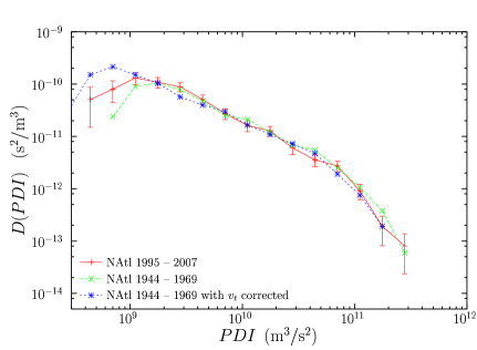
Figure 5: Probability density of tropical-cyclone $PDI$ for time periods with different levels of activity. (a) The comparison between 1971-1994 and 1995-2007 shows that in the latter period larger $PDI$ values are possible. (b) In contrast, the period 1944-1969 shows no significant differences with 1995-2007. Even, a correction of the speeds of the former period (subtracting 4 m/s Landsea93 ) does not change noticeably the results.

Figure 5(a) shows the $PDI$ distributions in the North Atlantic for the years 1971-1994 and 1995-2007. The first period corresponds predominantly to relatively low sea surface temperatures, whereas in the second period the temperatures are higher. We clearly see how the scale that delimits the boundary effects increases. In summary, the last years of the North Atlantic are characterized by larger hurricanes, in terms of dissipation of energy, in comparison with the period 1971-1994.

Nevertheless, going back beyond 1970 yields a different tendency, as then the hurricanes show a distribution very similar to that of recent years. In fact, Fig. 5(b) compares the $PDI$ distribution for the period 1944-1969 with the one corresponding to 1995-2007, showing no significant differences. Even a correction of old values of the speeds inspired in the work of Landsea Landsea93 ; Landsea_comment , in which they are decreased by an amount of 4 m/s, does not alter significantly the results.

7 Discussion

The criticality of tropical cyclones offers a new perspective for the understanding of this complex phenomenon. Naturally, many questions arise, and much more research will be necessary to answer them. First, we can wonder how this criticality relates to the results of Peters and Neelin Peters_np , who have recently proposed the criticality of the atmosphere for the transition to rainfall occurrence (i.e., the transition from no precipitation to precipitation). After all, tropical cyclones show, in addition to strong winds, enormous quantities of rainfall, and so they contribute to the precipitation data analyzed by Peters and Neelin. These authors showed that the state of the atmosphere, represented by its water-vapor content, is usually close to the onset of precipitation (this onset marks the critical point of the transition). However, tropical cyclones clearly surpass this onset of precipitation (O. Peters, private communication) and then it is not clear why they still retain critical characteristics.

A subsequent question is how the idea of criticality affects our vision of atmospheric processes, and, in particular, the concept of a chaotic weather Lorenz_book . It is true that both behaviors, chaos and criticality, share some characteristics, among them, an inherent unpredictability. But there are also fundamental differences. First, chaos usually appears in low-dimensional systems, i.e., systems described by a few non-linear differential equations, for instance, whereas criticality is the hallmark of a high number of strongly interacting degrees of freedom. And second, the unpredictability in chaos is described by the exponential separation of close trajectories (positive maximum Lyapunov exponent), whereas in a critical system this divergence should be a power law (with a zero maximum Lyapunov exponent, if one likes). This suggest that a reconsideration of the limits of predictability of the weather could give interesting outcomes Orrell .

8 Acknowledgements

The author was benefited by previous interaction with A. Ossó, made possible thanks to J. E. Llebot. Feedback from K. Emanuel, E. Fukada, J. Kossin, O. Peters, G. B. Raga, R. Romero, and A. Turiel was very valuable. Table 1 is based on a previous one by O. Peters and K. Christensen. Research projects 2009SGR-164, FIS2009-09508, and specially FIS2007-29088-E, from the EXPLORA - Ingenio 2010 program, have contributed in one form or another to the execution of the research.

References

- (1) In J. B. Elsner and T. H. Jagger, editors, Hurricanes and Climate Change. Springer, New York, 2009.
- (2) S. D. Aberson. Regimes or cycles in tropical cyclone activity in the North Atlantic. Bull. Am. Met. Soc., 90(1):39–43, 2009.
- (3) M. Baiesi, M. Paczuski, and A. L. Stella. Intensity thresholds and the statistics of the temporal occurrence of solar flares. Phys. Rev. Lett., 96:051103, 2006.
- (4) P. Bak. How Nature Works: The Science of Self-Organized Criticality. Copernicus, New York, 1996.
- (5) P. Bak, C. Tang, and K. Wiesenfeld. Self-organized criticality: an explanation of noise. Phys. Rev. Lett., 59:381–384, 1987.
- (6) G. D. Bell, M. S. Halpert, R. C. Schnell, R. W. Higgins, J. Lawrimore, V. E. Kousky, R. Tinker, W. Thiaw, M. Chelliah, and A. Artusa. Climate assessment for 1999. Bull. Am. Met. Soc., 81(6):S1–S50, 2000.
- (7) M. Bister and K. A. Emanuel. Dissipative heating and hurricane intensity. Meteorol. Atmos. Phys., 65:233–240, 1998.
- (8) S. M. Burroughs and S. F. Tebbens. Power-law scaling and probabilistic forecasting of tsunami runup heights. Pure Appl. Geophys., 162:331–342, 2005.
- (9) J. C. L. Chan. Comment on “Changes in tropical cyclone number, duration, and intensity in a warming environment”. Science, 311:1713b, 2006.
- (10) C. R. Chapman and D. Morrison. Cosmic Catastrophes. Plenum Press, New York, 1989.
- (11) K. Christensen, A. Corral, V. Frette, J. Feder, and T. Jøssang. Tracer dispersion in a self-organized critical system. Phys. Rev. Lett., 77:107–110, 1996.
- (12) K. Christensen and N. R. Moloney. Complexity and Criticality. Imperial College Press, London, 2005.
- (13) J.-H. Chu, C. R. Sampson, A. S. Levine, and E. Fukada. The Joint Typhoon Warning Center tropical cyclone best-tracks, 1945-2000. https://metocph.nmci.navy.mil/jtwc/besttracks/TCbtreport.html, 2002.
- (14) A. Clauset, C. R. Shalizi, and M. E. J. Newman. Power-law distributions in empirical data. SIAM Rev., 51:661–703, 2009.
- (15) A. Corral, A. Ossó, and J. E. Llebot. Scaling of tropical-cyclone dissipation. Nature Phys., 6:693–696, 2010.
- (16) A. Corral, L. Telesca, and R. Lasaponara. Scaling and correlations in the dynamics of forest-fire occurrence. Phys. Rev. E, 77:016101, 2008.
- (17) L. de Arcangelis, C. Godano, E. Lippiello, and M. Nicodemi. Universality in solar flare and earthquake occurrence. Phys. Rev. Lett., 96:051102, 2006.
- (18) J. B. Elsner, J. P. Kossin, and T. H. Jagger. The increasing intensity of the strongest tropical cyclones. Nature, 455:92–95, 2008.
- (19) K. Emanuel. Divine Wind: the History and Science of Hurricanes. Oxford University Press, New York, 2005.
- (20) K. Emanuel. Increasing destructiveness of tropical cyclones over the past 30 years. Nature, 436:686–688, 2005.
- (21) K. Emanuel. The hurricane-climate connection. Bull. Am. Met. Soc., (5):ES10–ES20, 2008.
- (22) V. Frette, K. Christensen, A. Malthe-Sørenssen, J. Feder, T. Jøssang, and P. Meakin. Avalanche dynamics in a pile of rice. Nature, 379:49–52, 1996.
- (23) S. B. Goldenberg, C. W. Landsea, A. M. Mestas-Nuñez, and W. M. Gray. The recent increase in Atlantic hurricane activity: Causes and implications. Science, 293:474–479, 2001.
- (24) W. M. Gray. General characteristics of tropical cyclones. In R. Pielke Jr. and R. Pielke Sr., editors, Storms, pages 145–163. Routledge, London, 2000.
- (25) W. M. Gray. Comments on “Increasing destructiveness of tropical cyclones over the past 30 years”. http://arxiv.org, 0601050, 2006.
- (26) W. M. Gray, C. W. Landsea, P. W. Mielke Jr., and K. J. Berry. Predicting Atlantic seasonal hurricane activity 6-11 months in advance. Wea. Forecast, 7:440–455, 1992.
- (27) T. E. Harris. The Theory of Branching Processes. Dover, New York, 1989.
- (28) S. Hergarten. Self-Organized Criticality in Earth Systems. Springer, Berlin, 2002.
- (29) B. R. Jarvinen, C. J. Neumann, and M. A. S. David. A tropical cyclone data tape for the North Atlantic basin, 1886-1983: contents, limitations, and uses. http://www.nhc.noaa.gov/pdf/NWS-NHC-1988-22.pdf, 1988.
- (30) H. J. Jensen. Self-Organized Criticality. Cambridge University Press, Cambridge, 1998.
- (31) Joint Typhoon Warning Center. https://metocph.nmci.navy.mil/jtwc/besttracks/index.html.
- (32) Y. Y. Kagan. Why does theoretical physics fail to explain and predict earthquake occurrence? In P. Bhattacharyya and B. K. Chakrabarti, editors, Modelling Critical and Catastrophic Phenomena in Geoscience, Lecture Notes in Physics, 705, pages 303–359. Springer, Berlin, 2006.
- (33) H. Kanamori and E. E. Brodsky. The physics of earthquakes. Rep. Prog. Phys., 67:1429–1496, 2004.
- (34) P. J. Klotzbach. Trends in global tropical cyclone activity over the past twenty years (1986 -2005). Geophys. Res. Lett., 33:L10805, 2006.
- (35) J. P. Kossin, K. R. Knapp, D. J. Vimont, R. J. Murnane, and B. A. Harper. A globally consistent reanalysis of hurricane variability and trends. Geophys. Res. Lett., 34:L04815, 2007.
- (36) F. Lahaie and J. R. Grasso. A fluid-rock interaction cellular automaton of volcano mechanics: Application to the Piton de la Fournaise. J. Geophys. Res., 103 B:9637–9650, 1998.
- (37) C. W. Landsea. A climatology of intense (or major) hurricanes. Mon. Weather Rev., 121:1703–1713, 1993.
- (38) C. W. Landsea. Hurricanes and global warming. Nature, 438:E11–E12, 2005.
- (39) C. W. Landsea. Counting Atlantic tropical cyclones back to 1900. Eos, 88 (18):197–202, 2007.
- (40) C. W. Landsea, B. A. Harper, K. Hoarau, and J. A. Knaff. Can we detect trends in extreme tropical cyclones? Science, 313:452–454, 2006.
- (41) E. N. Lorenz. The Essence of Chaos. University of Washington Press, Washington, 1993.
- (42) I. G. Main, L. Li, J. McCloskey, and M. Naylor. Effect of the Sumatran mega-earthquake on the global magnitude cut-off and event rate. Nature Geosci., 1:142, 2008.
- (43) B. D. Malamud. Tails of natural hazards. Phys. World, 17 (8):31–35, 2004.
- (44) B. D. Malamud, G. Morein, and D. L. Turcotte. Forest fires: An example of self-organized critical behavior. Science, 281:1840–1842, 1998.
- (45) National Hurricane Center. http://www.nhc.noaa.gov/tracks1851to2007atlreanal.txt, http://www.nhc.noaa.gov/tracks1949to2007epa.txt.
- (46) D. Orrell. Role of the metric in forecast error growth: how chaotic is the weather. Tellus, 54A:350–362, 2002.
- (47) O. Peters and K. Christensen. Rain viewed as relaxational events. J. Hidrol., 328:46–55, 2006.
- (48) O. Peters, C. Hertlein, and K. Christensen. A complexity view of rainfall. Phys. Rev. Lett., 88:018701, 2002.
- (49) O. Peters and J. D. Neelin. Critical phenomena in atmospheric precipitation. Nature Phys., 2:393–396, 2006.
- (50) J. M. Shepherd and T. Knutson. The current debate on the linkage between global warming and hurricanes. Geography Compass, 1:1–24, 2007.
- (51) D. Sornette. Critical Phenomena in Natural Sciences. Springer, Berlin, 2nd edition, 2004.
- (52) K. Trenberth. Uncertainty in hurricanes and global warming. Science, 308:1753–1754, 2005.
- (53) N. J. van der Elst and E. E. Brodsky. Connecting near and farfield earthquake triggering to dynamic strain. J. Geophys. Res., (submitted), 2010.
- (54) J. A. Wanliss and J. M. Weygand. Power law burst lifetime distribution of the SYM-H index. Geophys. Res. Lett., 34:L04107, 2007.
- (55) P. J. Webster, G. J. Holland, J. A. Curry, and H.-R. Chang. Changes in tropical cyclone number, duration, and intensity in a warming environment. Science, 309:1844–1846, 2005.
- (56) S. Zapperi, K. B. Lauritsen, and H. E. Stanley. Self-organized branching processes: Mean-field theory for avalanches. Phys. Rev. Lett., 75:4071–4074, 1995.