Variational and linearly-implicit integrators, with applications

Abstract

We show that symplectic and linearly-implicit integrators proposed by Zhang and Skeel [70] are variational linearizations of Newmark methods. When used in conjunction with penalty methods (i.e., methods that replace constraints by stiff potentials), these integrators permit coarse time-stepping of holonomically constrained mechanical systems and bypass the resolution of nonlinear systems. Although penalty methods are widely employed, an explicit link to Lagrange multiplier approaches appears to be lacking; such a link is now provided (in the context of two-scale flow convergence [61]). The variational formulation also allows efficient simulations of mechanical systems on Lie groups.

1 Introduction and main results

Integrators:

Symplectic integrators are popular for simulating mechanical systems due to their structure preserving properties (e.g., [18]). Implicit methods, on the other hand, allow accurate coarse time-stepping of a class of stiff or multiscale problems (e.g., [39, 14]). It is also a classical treatment to linearize implicit methods so that expensive nonlinear solves can be avoided (e.g., [4]). Although linearizations of most implicit symplectic methods are not symplectic, Zhang and Skeel found a family of symplectic and linearly-implicit integrators [70], which allows efficient and structure preserving simulations. We show that their method is not only symplectic but in fact variational.

Specifically, consider mechanical systems governed by Newton’s equation:

$$\dot{x}=v,\quad M\dot{v}=-\nabla V(x),$$ (1)

where $V\in\mathcal{C}^{2}(\mathbb{R}^{n})$ and $M$ is a $n\times n$ symmetric, positive-definite constant matrix.

If we consider the following discrete Lagrangian (see Section 2.1 for explanations):

$$\tilde{\mathcal{L}}_{d}(x_{k},x_{k+1},a_{k},a_{k+1})=h\Big{(}\frac{1}{2}\big{(}\frac{x_{k+1}-x_{k}}{h}\big{)}^{T}M\big{(}\frac{x_{k+1}-x_{k}}{h}\big{)}$$

$$-\frac{1}{2}\big{(}\beta h^{2}\frac{1}{2}a_{k}^{T}Ma_{k}+V(x_{k})+\beta h^{2}a_{k}^{T}\nabla V(x_{k})+\frac{1}{2}\beta^{2}h^{4}a_{k}^{T}\text{Hess}V(x_{k})a_{k}\big{)}$$

$$-\frac{1}{2}\big{(}\beta h^{2}\frac{1}{2}a_{k+1}^{T}Ma_{k+1}+V(x_{k+1})+\beta h^{2}a_{k+1}^{T}\nabla V(x_{k+1})+\frac{1}{2}\beta^{2}h^{4}a_{k+1}^{T}\text{Hess}V(x_{k+1})a_{k+1}\big{)}\Big{)},$$ (2)

then the Euler-Lagrange equation of the variational principle

$$\delta\sum_{k=1}^{N}\tilde{\mathcal{L}}_{d}(x_{k},x_{k+1},a_{k},a_{k+1})=0$$

yields the following symplectic method (originally stated in Section 3 in [70]):

Integrator 1.

Zhang and Skeel’s symplectic method (Z&S):

$$\begin{cases}x_{k+1}&=x_{k}+hv_{k}+\frac{1}{2}h^{2}f_{k}\\ v_{k+1}&=v_{k}+\frac{1}{2}h(f_{k}+f_{k+1})\\ a_{k}&=-M^{-1}\nabla V(x_{k})-M^{-1}\emph{Hess}V(x_{k})\beta h^{2}a_{k}\\ f_{k}&=a_{k}-\frac{1}{2}\beta^{2}h^{4}M^{-1}a_{k}\cdot V^{(3)}(x_{k})\cdot a_{k}\end{cases}$$ (3)

where $V^{(3)}(\cdot)$ is a 3rd-order tensor corresponding to 3rd-derivative of $V$, the symbol $\cdot$ stands for tensor contraction, and therefore $a_{k}\cdot V^{(3)}(x_{k})\cdot a_{k}$ is again a vector.

For computational efficiency, $a_{k}$ should be obtained by solving a symmetric linear system instead of inverting a matrix. In this sense, Z&S is linearly implicit.

Theorem 1.1.

Z&S is:

1. unconditionally linearly stable if $\beta\geq 1/4$.

2. variational (and thus symplectic and conserving momentum-maps).

3. 2nd-order convergent (if stable) and can be made arbitrarily high order convergent.

4. symmetric (“time-reversible”).

Showing Z&S is variational ensures, due to a discrete Noether theorem (e.g., [41] and [18]), that it also preserves momentum maps that correspond to system symmetries. This additional preservation property is desired in mechanical system simulations. The variational formulation also leads to a possible extension to Lie groups (Section 4.5).

Constrained dynamics:

One of our motivations for studying Z&S originates from a need for coarse time-steppings in penalty methods for constrained dynamics.

To model constrained dynamics, let

$$\mathcal{S}(q(t)):=\int_{a}^{b}\frac{1}{2}\dot{q}(t)^{T}M\dot{q}(t)-V(q(t))\,dt$$ (4)

be the action associated with system (1). Under a holonomic constraint $g(q)=0$, the system evolution coincides with the critical trajectory on the constraint manifold, i.e., the solution of:

$$\delta\mathcal{S}/\delta q=0\text{ and for all $t$, }q(t)\in g^{-1}(0).$$ (5)

This trajectory can also be obtained by solving the differential algebraic system

$$\begin{cases}M\ddot{q}=-\nabla V(q)+\lambda^{T}\nabla g(q)\\ g(q)=0\end{cases}$$ (6)

Penalty methods approximate rigid constraints by stiff potentials; this is a classical idea and we refer to [51, 59, 62, 48] for a non-comprehensive list of references. More precisely, modify the potential energy $V(q)$ to $V(q)+\frac{1}{2}\omega^{2}g(q)^{T}g(q)$, then the solution of (5) is approximated by the solution of the following unconstrained mechanical system:

$$M\ddot{q}^{\omega}=-\nabla V(q^{\omega})-\omega^{2}g(q^{\omega})^{T}\nabla g(q^{\omega}),$$ (7)

where $\omega$ is large enough. Paraphrasing [48], the problem is, “as a result of stiffness, the numerical differential equation solver takes very small time steps, using a large amount of computing time without getting much done”. Z&S alleviates this problem because it can use coarse time-steps and do not solve nonlinear systems (see Section 1.2).

On a related matter, although penalty methods are widely employed and proved convergent to constrained dynamics (see Section 1.1), a quantitative analysis of its link to Lagrange multiplier approach (6) appeared to be lacking. We show that the solution of (7) converges to that of (6) as $\omega\rightarrow\infty$ in the sense of two-scale Flow convergence (see Definition 1.1 in [61]). More precisely, we have (explained in Section 3; throughout this paper, ‘bounded’ means having a norm bounded by an $\omega$-independent constant):

Theorem 1.2.

Denote by $q^{\omega}(t)$ the solution to (7) with $q^{\omega}(0)=q_{0}$ and $\dot{q}^{\omega}(0)=\dot{q}_{0}$ (where $g(q_{0})=0$ and $\frac{d}{dt}g(q_{0})=\nabla g(q_{0})\cdot\dot{q}_{0}=0$). Suppose that $M$ is non-singular, $V(\cdot)$ is bounded from below, $V(q)$ diverges towards infinity as $|q|\rightarrow\infty$, $V(\cdot)$ and $g(\cdot)$ are $C^{2}$ with bounded derivatives, and for all $q\in g^{-1}(0)$, $\nabla g(q)$ has a constant rank equal to the codimension of the constraint manifold, then

$$\lambda(t):=-\lim_{T\rightarrow 0}\lim_{\omega\rightarrow\infty}\frac{1}{T}\int_{t}^{t+T}\omega^{2}g(q^{\omega}(s))\,ds$$ (8)

exists. Also, the solution $q(t)$ of

$$\begin{cases}M\ddot{q}(t)=-\nabla V(q(t))+\lambda(t)^{T}\nabla g(q(t))\\ g(q(t))=0,\qquad q(0)=q_{0},\qquad\dot{q}(0)=\dot{q}_{0}\end{cases}$$ (9)

exists and satisfies

$$q^{\omega}\xrightarrow{F}q$$ (10)

in the sense of two-scale Flow convergence [61], i.e., for all bounded $t\geq 0$ and all bounded and uniformly Lipschitz continuous test function $\varphi$,

$$\lim_{T\rightarrow 0}\lim_{\omega\rightarrow\infty}\frac{1}{T}\int_{t}^{t+T}\varphi(q^{\omega}(s))-\varphi(q(s))\,ds=0$$ (11)

Outline of the paper:

Section 2 derives Z&S from a variational principle, relates it to Newmark integrators, and discusses its properties. Section 3 illustrates how penalty methods converge to Lagrange multiplier approach. Section 4 applies the method to constrained systems (pendula and water molecular dynamics), a non-constrained model of DNA division, and a mechanical system on SO(3) illustrating the benefits of a variational formulation.

1.1 On penalty methods

The penalty strategy of replacing holonomic constraints by stiff potentials is widely used. For example, it is a common treatment in computer graphics (e.g., [62, 67, 48]).

It is known that the penalized solution converges to constrained dynamics in $C^{1}$ topology, as long as its initial condition is in tangent bundle of the constraint manifold. We refer to, e.g., the pioneering work of [51, 59], to [7, 5, 56] for recent progress, and to Chapter XIV.3 of [18] for a review.

The reverse point of view has also been employed, particularly in molecular dynamics, where stiff oscillatory molecular bonds are replaced by rigid constraints for the purpose of allowing larger time-steps (e.g., [15, 54]). If the initial velocity is not in the tangent plane then a correction potential might also be required to account for the non-zero normal energy (e.g., [15, 49, 55]). The Fixman potential [15] is a classical example of such a correction, in particular when investigating thermodynamic properties of molecular systems (see e.g., [3]); on the other hand, [6] suggests that Fixman might not be the right correction for deterministic systems.

1.2 One constrained dynamics

Other popular constrained dynamics methods include: generalized coordinates on the constraint manifold (e.g., [27]) and Lagrange multipliers (e.g., SHAKE [52], RATTLE [2], SETTLE [21], LINCS [44], M-SHAKE [34]). The equivalence between these two approaches is well-established (e.g., [66]). These numerical methods allow an $o(1)$ integration step, but they also require solving nonlinear systems at each step. Unfortunately, linearization of these methods are no longer symplectic, and therefore resorting to linearization for a speed-up is at the risk of losing long-time accuracy.

The advantage of using a penalty approach depends on the system: if the system has a large number of coupled constraints, then an integration of the penalized system, even with small steps, would still be faster than generalized coordinate and Lagrange multiplier methods, which require solving high dimensional nonlinear systems.

Z&S provides a compromise by allowing large integration steps ($o(1)$, independent of $\omega$) with limited cost of a linear solve per iteration. It remains accurate when applied to penalized system (7), even though the $o(1)$ step does not resolve stiffness of the equation. This is because stiffness in this system results in fast oscillations non-tangent to a stable slow manifold (Section 3). Although implicit methods damp high frequencies in oscillations (e.g., [19]), the approximation of fast oscillations by slower ones (as in [39]) is sufficient for the approximation of slow dynamics on the constraint manifold.

We refer to M-SHAKE [34] for an example of recent developments to the Lagrange multiplier method. While M-SHAKE is limited to systems with distance constraints, Z&S combined with penalty method can implement arbitrary holonomic constraints.

2 Z&S: structure-preserving and stable integrators

2.1 Derivation from Newmark integrators

The Newmark family of algorithms are extensively used in structural dynamics [46]:

Integrator 2.

Newmark:

$$\begin{cases}q_{k+1}&=q_{k}+h\dot{q}_{k}+\frac{h^{2}}{2}[(1-2\beta)a_{k}+2\beta a_{k+1}]\\ \dot{q}_{k+1}&=\dot{q}_{k}+h[(1-\gamma)a_{k}+\gamma a_{k+1}]\\ a_{k}&=-M^{-1}\nabla V(q_{k})\end{cases}$$ (12)

Newmark is generally implicit when $\beta\neq 0$. When $\gamma=1/2$, it is 2nd-order accurate and variational [30], and we restrict ourselves to this case in this paper. Integrator 12 does not preserve the canonical symplectic form, and it was shown [58, 41] that if one pushes forward the update map by a coordinate transform $\eta:TQ\rightarrow TQ$ defined as

$$(x,v):=\eta(q,\dot{q})=(q+\beta h^{2}M^{-1}\nabla V(q),\dot{q})\quad,$$ (13)

then we obtain an integrator that preserves the canonical symplectic form on $T^{*}Q$:

Integrator 3.

Push-forward Newmark:

$$\begin{cases}x_{k+1}&=x_{k}+hv_{k}+\frac{1}{2}h^{2}a_{k}\\ v_{k+1}&=v_{k}+\frac{1}{2}h(a_{k}+a_{k+1})\\ a_{k}&=-M^{-1}\nabla V(x_{k}+\beta h^{2}a_{k})\end{cases}$$ (14)

These two methods are unconditionally linearly stable if $\beta\geq 1/4$ [11, 58]. Newmark with $\beta\geq 1/4$ is known to be nonlinearly stable under specific conditions [24], and Push-forward Newmark is known to be stable near stable fixed points in non-resonant nonlinear settings [57]. Nevertheless, there are nonlinear cases in which Newmark is no longer stable [12, 35]. In fact, few convergent methods are unconditionally stable for arbitrary nonlinear systems to the authors’ knowledge (see also [68]).

Now, consider the following discrete Lagrangian (see [41] for a review of variational integrators and [1] for one of many excellent reviews of analytical mechanics):

$$\mathcal{L}_{d}(x_{k},x_{k+1},a_{k},a_{k+1})=h\Big{(}\frac{1}{2}\big{(}\frac{x_{k+1}-x_{k}}{h}\big{)}^{T}M\big{(}\frac{x_{k+1}-x_{k}}{h}\big{)}-\frac{1}{2}\big{(}\beta h^{2}\frac{1}{2}a_{k}^{T}Ma_{k}+V(x_{k}+\beta h^{2}a_{k})\big{)}$$

$$\qquad\qquad-\frac{1}{2}\big{(}\beta h^{2}\frac{1}{2}a_{k+1}^{T}Ma_{k+1}+V(x_{k+1}+\beta h^{2}a_{k+1})\big{)}\Big{)},$$ (15)

then, (14) is the associated Euler-Lagrange equation, i.e., the critical point of discretized action $\sum_{k}\mathcal{L}_{d}(x_{k},x_{k+1},a_{k},a_{k+1})$. Note this variational formulation is explicit and distinct from the one implicitly defined in [41].

However, (15) is still implicit. Therefore we use a 2nd order Taylor expansion of (15) and derive (2). To obtain the corresponding discrete Euler-Lagrange equation, we compute $\partial\tilde{\mathcal{L}}_{d}/\partial a_{k}=0$, which leads to

$$Ma_{k}+\nabla V(x_{k})+\beta h^{2}\text{Hess}V(x_{k})a_{k}=0.$$ (16)

We then compute the discrete Legendre transform (see [41] for notation and terminology), which introduces the momentum and leads to

$$\begin{cases}p_{k}&=-D_{1}L_{d}(x_{k},x_{k+1},a_{k},a_{k+1})\\ &=M\frac{x_{k+1}-x_{k}}{h}+\frac{h}{2}\left(-Ma_{k}+\frac{1}{2}\beta^{2}h^{4}a_{k}\cdot V^{(3)}(x_{k})\cdot a_{k}\right)\\ p_{k+1}&=D_{2}L_{d}(x_{k},x_{k+1},a_{k},a_{k+1})\\ &=M\frac{x_{k+1}-x_{k}}{h}-\frac{h}{2}\left(-Ma_{k+1}+\frac{1}{2}\beta^{2}h^{4}a_{k+1}\cdot V^{(3)}(x_{k+1})\cdot a_{k+1}\right)\end{cases}$$ (17)

Since the velocity and momentum are related via $v_{k}=M^{-1}p_{k}$, we obtain the Z&S update (3).

Because the new discrete Lagrangian $\tilde{\mathcal{L}}_{d}$ is quadratic in $a$, nonlinear solves in Push-forward Newmark are replaced by linear solves in Z&S. Consequently, Z&S exhibits a speed advantage. Numerical illustrations of this advantage are in Section 4.

2.2 On Z&S

Linearizing equations:

Z&S is obtained as the linearization of Push-forward Newmark update map combined with a small correction. More precisely, the Taylor expansion of Line 3 of (14) leads to (16), and Lines 1-2 in (14) can be rewritten in terms of momentum as

$$\begin{cases}p_{k}&=-D_{1}L_{d}(x_{k},x_{k+1},a_{k},a_{k+1})\\ &=M\frac{x_{k+1}-x_{k}}{h}+\frac{h}{2}\left(-Ma_{k}\right)\\ p_{k+1}&=D_{2}L_{d}(x_{k},x_{k+1},a_{k},a_{k+1})\\ &=M\frac{x_{k+1}-x_{k}}{h}-\frac{h}{2}\left(-Ma_{k+1}\right)\end{cases}$$

The difference are two $\mathcal{O}(h^{5})$ terms (corresponding to $\frac{1}{4}\beta^{2}h^{5}a\cdot V^{(3)}(x)\cdot a$). To be consistent with the literature, we summarize this variant using velocity instead of momentum:

Integrator 4.

Zhang and Skeel’s method simplified (Z&Ss):

$$\begin{cases}x_{k+1}&=x_{k}+hv_{k}+\frac{1}{2}h^{2}a_{k}\\ v_{k+1}&=v_{k}+\frac{1}{2}h(a_{k}+a_{k+1})\\ a_{k}&=-(M+\emph{Hess}V(x_{k})\beta h^{2})^{-1}\nabla V(x_{k})\end{cases}$$ (18)

Theorem 2.1.

Z&Ss is:

1. unconditionally linearly stable if $\beta\geq 1/4$.

2. symplectic, if the $n\times n$ matrix $M+\emph{Hess}V(x)\beta h^{2}$ commutes with the $n\times n$ matrix $V^{(3)}(x)\cdot(M+\emph{Hess}V(x)\beta h^{2})^{-1}\cdot\nabla V(x)$ ($\cdot$ is tensor contraction).

3. 2nd-order convergent (if stable) and can be made arbitrarily high order convergent.

4. symmetric (“time-reversible”).

Z&Ss is not always symplectic due to the removal of $\mathcal{O}(h^{5})$ terms. However, it requires no high-order tensor operations and is thus a good choice for high-dimensional problems.

Partial Newton solve:

Line 3 of Z&Ss can be viewed as executing only the first step of a Newton solver for the nonlinear equation $a_{k}=-M^{-1}\nabla V(x_{k}+\beta h^{2}a_{k})$.

Preconditioning, filtering and regularization:

The factor of $(M+\text{Hess}V(x)\beta h^{2})^{-1}$ in front of $\nabla V(x)$ can be thought as an optimization preconditioner or a way to filter [22, 13] / regularize [16, 53] high frequency oscillations.

2.3 Properties

(Proofs of results introduced in this paragraph are standard and available online at http://www.math.gatech.edu/~mtao/TaOw14_supplemental.pdf).

Theorem 2.2 (Stability).

Z&S (Integrator 3) is unconditionally linearly stable if and only if $\beta\geq 1/4$.

The proof of the unconditional linearly stability (for $\beta\geq 1/4$) of Integrators 18 and 3 are similar. If the potential is of form $V(x)=V_{0}(x)+\epsilon^{-1}V_{1}(x)$, then the following modification of Z&Ss is unconditionally linearly stable as long as $\beta>1/4+\mathcal{O}(\epsilon)$:

Integrator 5.

Simplified Z&Ss for stiff systems ($\epsilon^{-1}\gg 1$):

$$\begin{cases}x_{k+1}&=x_{k}+hv_{k}+\frac{1}{2}h^{2}a_{k}\\ v_{k+1}&=v_{k}+\frac{1}{2}h(a_{k}+a_{k+1})\\ a_{k}&=-M^{-1}(\nabla V_{0}(x_{k})+\epsilon^{-1}\nabla V_{1}(x_{k}))-M^{-1}\epsilon^{-1}\emph{Hess}V_{1}(x_{k})\beta h^{2}a_{k}\end{cases}$$ (19)

Theorem 2.3 (Consistency).

Consider an integrator for (1) given by:

$$\begin{cases}x_{k+1}&=x_{k}+hv_{k}+\frac{1}{2}h^{2}a_{k}\\ v_{k+1}&=v_{k}+\frac{1}{2}h(a_{k}+a_{k+1}+h^{4}g(x_{k})+h^{4}g(x_{k+1}))\\ a_{k}&=-M^{-1}\nabla V(x_{k})-M^{-1}f(x_{k})h^{2}a_{k}\end{cases},$$ (20)

where $f,g\in\mathcal{C}(Q)$ are arbitrary functions. If $V\in\mathcal{C}^{3}(Q)$, this integrator has 3rd order truncation error.

Corollary 2.1.

Z&S (Integrator 3), Z&Ss (Integrator 18) and simplified Z&Ss for stiff systems (Integrator 19) are 2nd order convergent, provided stability.

Symmetry (i.e., time-reversibility) is one desired property of numerical integrators, because it leads to good long time performance (see for instance [18] or [37]).

Theorem 2.4 (Symmetry / Time-Reversibility).

Let $f\in\mathcal{C}^{1}(Q)$ is an arbitrary function. The integrator defined by

$$\begin{cases}x_{k+1}&=x_{k}+hv_{k}+\frac{1}{2}h^{2}f_{k}\\ v_{k+1}&=v_{k}+\frac{1}{2}h(f_{k}+f_{k+1})\\ f_{k}&=f(x_{k})\end{cases},$$ (21)

is symmetric (time-reversible).

Corollary 2.2.

Z&S (Integrator 3) is symmetric (time-reversible).

Remark 2.1.

Arbitrary high order Z&S can be obtained using standard splitting schemes as in [69, 45, 18]. A 4th-order example is provided in the supplemental material.

Theorem 2.5.

Z&S (Integrator 3) is symplectic.

Lemma 2.1 (Symplecticity).

Consider an integrator given by (21). If $f\in\mathcal{C}^{1}(Q)$ is a function with symmetric Jacobian, then this integrator is symplectic.

Remark 2.2.

The commutation condition in Theorem 2.1 ensures a symmetric Jacobian and hence the symplecticity of Z&Ss. Two very special cases where this condition is satisfied are: when the system contains only 1 degree of freedom, or when $\text{Hess}(V)$ can be diagonalized by a matrix independent of $x$.

Remark 2.3.

Fully-nonlinear implicit symplectic methods (e.g., midpoint or Newmark) are not exactly symplectic due to numerical errors in nonlinear solves, which are oftentimes much larger than those in linear solves.

3 Lagrange multiplier methods as limits of penalty methods

Lagrange multiplier and penalty methods respectively simulate (6) and (7). It is known (Section 1.1 and 1.2) that both are equivalent to constrained dynamics (in the $\omega\rightarrow\infty$ limit). We now quantify the equivalence between themselves.

First observe that this equivalence is not necessarily achieved via

$$\lambda(t)=-\lim_{\omega\rightarrow\infty}\omega^{2}g(q^{\omega}(t))$$ (22)

Consider for instance $V=0$, $g(q)=q$, $q^{\omega}(0)=1/\omega^{2}$ and $p^{\omega}(0)=0$; (7) leads to $q^{\omega}(t)=\cos(\omega t)/\omega^{2}$, and (6) yields $q(t)=0$ and $\lambda(t)=0$, but then (22) cannot hold because $\lim_{\omega\rightarrow\infty}\omega^{2}g(q^{\omega}(t))$ does not exist.

The appropriate notion of equivalence is provided Theorem 11. The idea is as follows: energy conservation implies that $g(q^{\omega})$ is at most $\mathcal{O}(1/\omega)$ (see Lemma 6.1). In fact, $g(q^{\omega})$ can be further shown to be $\mathcal{O}(1/\omega^{2})$ (see Remark 6.1 or [31]), and constraints are satisfied with small errors that oscillate rapidly. To describe the Lagrange multiplier system (6) as a limit of penalized systems (7), the convergence of these fast oscillations should be understood in a weak sense, whereas slow dynamics on the constrained manifold converges strongly. Thus we employ two-scale Flow convergence (Eq.11) for this description. Convergence is first proved for flat constraint manifold (Lemma 41), and then local charts are patched together (see Appendix); this leads to Theorem 11.

Remark 3.1.

If the limit in (22) exists, then (8) simplifies to (22) and two-scale F-convergence becomes strong convergence. However, we are not aware of a practical example where such a limit exists.

4 Application examples

Z&S (Integrator 3) is applied in Sections 4.1,4.2 and 4.4; Section 4.3 employs simplified Z&Ss for stiff system (Integrator 19) due to its efficiency for high-dimensional systems; Section 4.5 is based on variational formulation (2).

Speed comparisons are provided in terms of running times (using Matlab 7.7 on an Intel Core 2 Duo 2.4G laptop, with nonlinear solver of ‘fsolve’); however, these numbers are machine and platform dependent (e.g., Matlab is very well-optimized for linear algebra), and should serve only as a qualitative illustration of efficiencies.

4.1 Double pendulum

Implementation:

One way to represent planar double pendulum is to use 4 degrees of freedom and 2 nonlinear constraints. Using the notations of (7), we have

$$M=\begin{bmatrix}m_{1}&0&0&0\\ 0&m_{1}&0&0\\ 0&0&m_{2}&0\\ 0&0&0&m_{2}\end{bmatrix},\qquad\begin{aligned} &V(x_{1},y_{1},x_{2},y_{2})=-\text{g}y_{1}-\text{g}y_{2},\\ &g(x_{1},y_{1},x_{2},y_{2})=\begin{bmatrix}x_{1}^{2}+y_{1}^{2}-L_{1}^{2}\\ (x_{2}-x_{1})^{2}+(y_{2}-y_{1})^{2}-L_{2}^{2}\end{bmatrix}.\end{aligned}$$

For simplicity, we adopt a dimensionless convention and assume $m_{1}=m_{2}=\text{g}=1$.

The Z&S simulation of the penalized system (7) is straightforward. SHAKE [52] is used as the Lagrangian multiplier method in our experiments; it is nonlinearly implicit.

Symplectic integration in generalized coordinates $\theta,\phi$ ($x_{1}=L_{1}\sin\theta$, $y_{1}=-L_{1}\cos\theta$, $x_{2}=L_{1}\sin\theta+L_{2}\sin\phi$, $y_{2}=-L_{1}\cos\theta-L_{2}\cos\phi$) is also implicit. This is because, after writing down the Lagrangian, one will note a position-dependent mass matrix of

$$\tilde{M}(\theta,\phi)=\begin{bmatrix}2L_{1}^{2}&L_{1}L_{2}(\cos\theta\cos\phi+\sin\theta\sin\phi)\\ L_{1}L_{2}(\cos\theta\cos\phi+\sin\theta\sin\phi)&L_{2}^{2}\end{bmatrix},$$ (23)

Consequently, even the most well known “explicit” variational integrators such as variational Euler (i.e., leapfrog) and Velocity-Verlet, will be implicit.

Note although $g$ is quadratic, the penalized ODE is cubically nonlinear.

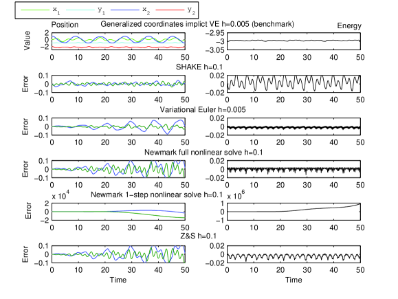
Figure 1: Errors of SHAKE, Variational Euler on the penalized system, Newmark (with nonlinear systems fully solved), linearly-implicit Newmark (with only 1st iteration of nonlinear solve at each step), and Z&S. Benchmark is provided by small step Variational Euler in generalized coordinates. Initial conditions are $x_{1}(0)=0,y_{1}(0)=-1,x_{2}(0)=1,y_{2}(0)=-2$, zero momenta; $L_{1}=1$ and $L_{2}=\sqrt{2}$. $\omega=20$ in Rows 3-6. $\beta=0.4$. Row 3 uses $h=0.1/\omega$ for stability, and Row 2,4,5,6 use a 20x bigger $h=0.1$. Position errors are only shown on $x_{2}$ and $y_{2}$ for readability.

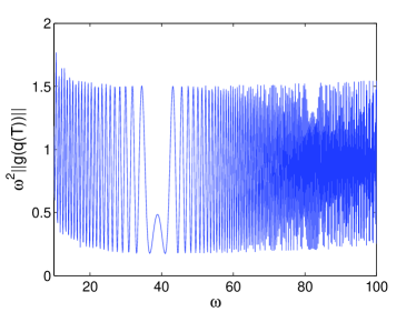
(a) $\omega^{2}\|g(q(T))\|$ numerically computed as a function of $\omega$. $T=50$ fixed.

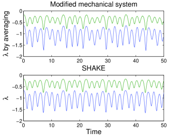
(b) Lagrange multipliers computed by (8) from $\omega=20$ penalized system and by SHAKE. The integral in (8) is approximated by empirical average over time window of width 0.2.

Figure 2: Satisfaction of constraints and Lagrangian multiplier. Z&S with $h=0.01$ is used (for smooth curve; Verlet would require $h=0.001$ for stability); other parameters are same as in Figure 1.

Results:

Figure 1 illustrates errors of different methods. Newmark (Integrator 12) with only 1st step of nonlinear solve (Row 5) has a large error due to the loss of symplecticity, even though the method is still consistent. On the contrary, Z&S (Row 6) yields small errors almost identical to those of fully-nonlinear-solve Newmark (Row 4).

Z&S produces larger error than SHAKE, because there is modeling error due to finite $\omega$ in addition to integration error (Row 3). We chose an intermediate $\omega$, which is sufficiently large to approximate the constraints, yet small enough to show that the penalized system is only an approximation. A larger $\omega$ leads to a more accurate approximation, but if it is too large, e.g., $\omega=2000$ (i.e., a stiffness of $\omega^{2}=4\times 10^{6}$), instability occurs in all Z&S, original Newmark, and implicit midpoint due to strong nonlinearity.

If $\omega$ is finite, the approximation error is predicted to be $\mathcal{O}(\omega^{-2})$ (Remark 6.1). See Figure 2(a) for a numerical illustration. Figure 2(b) compares the Lagrange multiplier computed by SHAKE with the one obtained from the penalized system via Theorem 11. There is no strong convergence but only a 2-scale F-convergence.

It is known that the double pendulum contains a chaotic region (e.g., [50]). Variational integrator is desired for simulating such systems [10, 42]. None of our symplectic simulations (Row 1,2,3,4,6) led to numerical leakage between regular and chaotic regions.

Generalized coordinate implicit VE (benchmark), SHAKE, Variational Euler, Newmark with full nonlinear solve, Newmark with one-step nonlinear solve, and Z&S respectively spent 91.3, 3.8, 1.0, 5.3, 0.2 (2.6 if $\text{Hess}V$ is not analytically provided but approximated by the nonlinear solver), and 0.4 seconds on the above simulation.

4.2 A simple high-dimensional example: a chain of many pendula

Consider a chain of $n$ pendula, which approximates a continuous rope. The system is similarly modeled by (7) with

$$M=\begin{bmatrix}1&0&\cdots&0&0\\ 0&1&\cdots&0&0\\ \vdots&\vdots&\ddots&\vdots&\vdots\\ 0&0&\cdots&1&0\\ 0&0&\cdots&0&1\end{bmatrix},\quad\begin{aligned} &V(x_{1},y_{1},\cdots,x_{n},y_{n})=-\sum_{i=1}^{n}y_{i},\\ &g(x_{1},y_{1},\cdots,x_{n},y_{n})=\begin{bmatrix}x_{1}^{2}+y_{1}^{2}-L_{1}^{2}\\ (x_{2}-x_{1})^{2}+(y_{2}-y_{1})^{2}-L_{2}^{2}\\ \vdots\\ (x_{n}-x_{n-1})^{2}+(y_{n}-y_{n-1})^{2}-L_{n}^{2}\end{bmatrix}.\end{aligned}$$

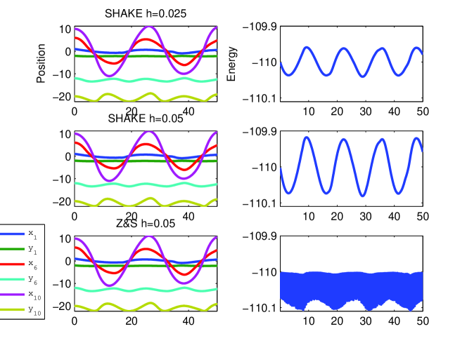
Figure 3: Simulations by SHAKE with $h=0.05$ and $h=0.025$ and by Z&S with $h=0.05$ on $\omega=20$ penalized system. $n=10$; $x_{i}(0)=i,y_{i}(0)=-2i$ for $i=1,\ldots,n$ and initial momenta are zero; $L_{i}=\sqrt{5}$; $\beta=0.4$. For clarity, not all degrees of freedom are shown.

Figure 3 shows good agreement between SHAKE and Z&S (trajectories instead of errors are shown due to lack of accurate benchmark — an analytical solution is unavailable, and Lagrange multiplier formulations and generalized coordinate approaches involve solving large nonlinear systems). SHAKE with $h=0.025$, $h=0.05$, and Z&S with $h=0.05$ respectively spent 16.5, 8.1, and 1.1 seconds in these simulations.

4.3 Molecular dynamics of water cluster

Consider the dynamics of water molecules, each interacting with others via non-bonded interactions of electrostatic and van der Waals forces (both highly nonlinear).

Water model:

Use the popular TIP3P model (e.g., [28])). Let $q_{ai}$ and $p_{ai}$ be position and momentum of $a$th molecule’s $i$th atom (both 3-vectors). The Hamiltonian is:

$$\mathcal{H}=\sum_{a=1}^{N}\sum_{i=1}^{3}\frac{1}{2}p_{ai}^{T}m_{i}^{-1}p_{ai}+\sum_{a=1}^{N-1}\sum_{b=a+1}^{N}\left(\sum_{i=1}^{3}\sum_{j=1}^{3}\frac{K_{c}Q_{i}Q_{j}}{r_{ai,bj}}+\frac{A}{r_{a2,b2}^{12}}-\frac{C}{r_{a2,b2}^{6}}\right),$$ (24)

where $r_{ai,bj}:=\|q_{ai}-q_{bj}\|$ is inter-atom distance, $m_{1}=m_{3}$ are hydrogen mass and $m_{2}$ oxygen, $K_{c}$ is electrostatic constant, $Q_{i}$ is partial charge of atom $i$ relative to electron charge, $A$ and $C$ are Lennard-Jones constants that approximate van der Waals forces.

In this TIP3P model (or many other prevailing models such as SPC, BF, TIPS2, and TIP4P, which are discussed in, e.g., [28, 64]), each water molecule is considered as a rigid body, with two O-H bond lengths and H-O-H bond angle fixed as constants $r_{OH}$ and $\alpha_{HOH}$. Detailed values of these model parameters could be found in, e.g., [28].

Therefore, the following vectorial constraint enforces the geometry of molecules:

$$g(q)=\begin{bmatrix}(q_{11}-q_{12})(q_{11}-q_{12})^{T}-r_{OH}^{2}\\ (q_{13}-q_{12})(q_{13}-q_{12})^{T}-r_{OH}^{2}\\ (q_{11}-q_{13})(q_{11}-q_{13})^{T}-r_{HH}^{2}\\ \vdots\\ (q_{N1}-q_{N2})(q_{N1}-q_{N2})^{T}-r_{OH}^{2}\\ (q_{N3}-q_{N2})(q_{N3}-q_{N2})^{T}-r_{OH}^{2}\\ (q_{N1}-q_{N3})(q_{N1}-q_{N3})^{T}-r_{HH}^{2}\end{bmatrix},$$ (25)

where $r_{HH}:=2r_{OH}\sin(\alpha_{HOH}/2)$ is a constant. This leads to penalized Hamiltonian

$$\tilde{\mathcal{H}}=\mathcal{H}+\frac{1}{2}\omega^{2}\sum_{a=1}^{N}\left((r_{a1,a2}^{2}-r_{OH}^{2})^{2}+(r_{a3,a2}^{2}-r_{OH}^{2})^{2}+(r_{a1,a3}^{2}-r_{HH}^{2})^{2}\right).$$ (26)

Constant temperature simulation:

Constant temperature simulations are of practical importance because (i) thermal fluctuations are an indispensable component of molecular dynamics, and (ii) the N-body system is chaotic and its long-time deterministic simulation has limited predictive power. We use Langevin dynamics (e.g., [54]) as our constant temperature model.

In this model, molecules experience perturbation by noise and dissipation due to friction, and the dynamics can be expressed by the following SDEs:

$$\begin{cases}dq=\frac{\partial\tilde{\mathcal{H}}}{\partial p}\,dt\\ dp=-\frac{\partial\tilde{\mathcal{H}}}{\partial q}\,dt-\gamma\frac{\partial\tilde{\mathcal{H}}}{\partial p}\,dt+\sqrt{2\gamma\beta^{-1}}dW\end{cases},$$ (27)

where $W$ is a $9N$-dimensional Wiener process, $\beta^{-1}>0$ is the constant temperature, and $\gamma>0$ is dissipation strength. The system admits an invariant measure of Boltzmann-Gibbs (BG; also known as the canonical ensemble), given by:

$$\pi(q,p)=Z^{-1}\exp(-\beta\tilde{\mathcal{H}}),$$ (28)

where $Z=\int_{\mathbb{R}^{18N}}\exp(-\beta\tilde{\mathcal{H}})\,dq\,dp$ is the partition function.

To simulate (27), we use the Geometric Langevin Algorithm (GLA; see [9]). GLA allows for an extension of Hamiltonian integrators to Langevin integrators. It is a splitting scheme, based on composing the one-step update of a determinstic integrator with the exact flow of an Ornstein-Uhlenbeck process (OU for short, given by $dp=-\gamma M^{-1}p\,dt+\sqrt{2\gamma\beta^{-1}}dW$, i.e., driftless noise and friction). It has been shown [9] that if the deterministic integrator is symplectic, then GLA not only provides a good approximation of trajectories but also of BG (the invariant distribution). In this example, the deterministic building block is simplified Z&Ss (Integrator 19) or SHAKE.

Constant temperature molecular dynamics is a rich research field, and our investigation will only be numerical. The thermodynamic properties of a system with strong restraint may not be equivalent to those of a constrained system (e.g., [3]); the Fixman potential is a classical way to correct the difference (see [47] for debate on the validity of this correction). Proving that a numerical method samples a good approximation of the invariant distribution is nontrivial. [9] combines ergodicity with the backward error analysis of symplectic integrators to show that the invariant distribution is preserved with a high order of accuracy. It is conjectured (Remark 2.1 in [9]) that SHAKE+GLA approximately samples a constrained BG distribution

$$\hat{\pi}(q,p)=\hat{Z}^{-1}\exp(-\beta\mathcal{H}),$$ (29)

where $\hat{Z}=\int_{T^{*}g^{-1}(0)}\exp(-\beta\mathcal{H})\,dq\,dp$. Relating (28) and (29) is left as a future investigation. See [65, 3, 20, 38] for more about finite temperature constrained dynamics.

Numerical results:

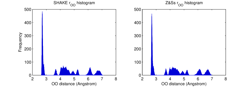
Figure 4: Empirical OO radial distribution in 7-water cluster obtained by long time ($T=10000$) simulations of SHAKE and simplified Z&Ss.

One quantity of interest in water cluster is the distribution of interatomic oxygen-oxygen distances in the thermal equilibrium limit, also known as the OO radial distribution [28]. To illustrate the accuracy of Z&S in sampling BG, Figure 4 shows histograms obtained by long time simulations of SHAKE and simplified Z&Ss (Integrator (19)) that approximate this distribution. We chose a system of size $N=7$ (i.e., $63$ degrees of freedom) so that peaks in the distribution could be clearly distinguished. SHAKE required 13472 secs, including 12284 secs on nonlinear solves (with tolerances of $10^{-6}$ on variable and $10^{-10}$ on function value), whereas simplified Z&Ss used 1549 secs, including 67 secs on linear solves. Parameters are $\omega=20$, $h=0.05$ in both simulations, $\gamma=0.01$ and $\beta=50$.

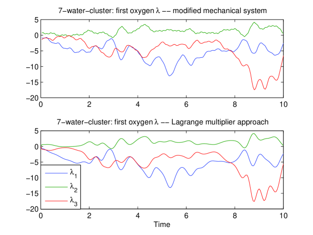
Figure 5: Lagrange multipliers from the penalized system (simplified Z&Ss) and by SHAKE. Only 1st oxygen atom is shown, and illustration is terminated before chaos. Empirical average uses a time window of width 0.2. $\omega$ temporarily enlarged to $500$ for clearer visualization of details.

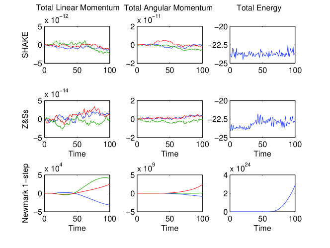
Figure 6: Energy, linear and angular momentum preservation by simplified Z&Ss, SHAKE, and partially-solved Newmark. $h=0.05$ for all. For clarity plots are drawn with a 20:1 downsample rate.

We also provide two deterministic simulations (with noise and friction turned off; other parameters remains unchanged unless indicated otherwise): (i) Figure 5 compares Lagrange multipliers computed by SHAKE and from the penalized system to illustrate Theorem 11. (ii) Figure 6 compares simplified Z&Ss, SHAKE, and partially solved Newmark (non-symplectic) in terms of energy and momentum conservations. Simplified Z&Ss lost symplecticity due to simplification, but it still exhibits improved preservation properties comparing to partially solved Newmark.

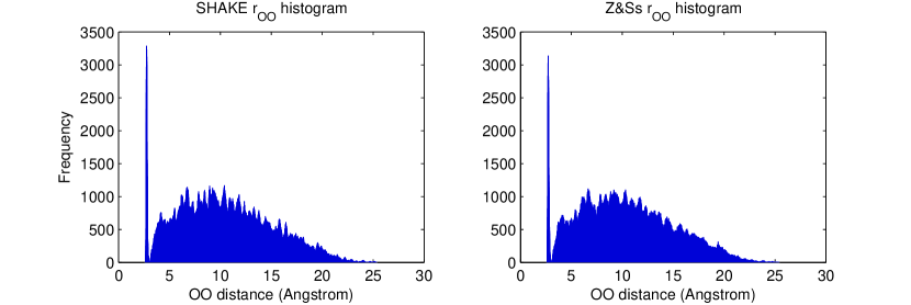
Figure 7: Empirical OO radial distribution in 100-water cluster obtained by simulations of SHAKE and simplified Z&Ss till $T=1000$.

To test scalability, we increase $N$ to $100$ ($900$ degrees of freedom) and illustrate results in Figure 7. SHAKE spent 42234 secs, including 14272 secs on solving nonlinear systems, and $\sim$28000 secs on computing $V$ and $\nabla V$, whereas simplified Z&Ss spent 30059 secs, including 319 secs on solving linear systems, and $\sim$29000 secs on $V$, $\nabla V$ and $\text{Hess}\,V$.

Efficiency of force evaluation:

Although simplified Z&Ss accelerates updates by linearization, for large systems the computational bottleneck is likely to be on force evaluations but not updates. Fortunately, significant progress has been made to accelerate force evaluations, such as the fast multipole method [17], or simply the idea of ignoring weak long-range forces. We did not employ any of them, but they can be used in adjunct to simplified Z&Ss.

Times spent on force evaluations by SHAKE and simplified Z&Ss are comparable; Hessian computations in simplified Z&Ss didn’t incur much overhead. This is because the potential is a function of relative distances $r_{ij}=\|x_{i}-x_{j}\|$. For such $f$,

$$\frac{\partial^{2}f(r)}{\partial x_{i}\partial x_{j}}=\frac{\partial r}{\partial x_{i}}\frac{\partial^{2}f}{\partial r^{2}}\frac{\partial r}{\partial x_{j}}+\frac{\partial f}{\partial r}\frac{\partial^{2}r}{\partial x_{i}\partial x_{j}},$$ (30)

but $\frac{\partial r}{\partial x}$ and $\frac{\partial f}{\partial r}$ are already computed when calculating the gradient, $\frac{\partial^{2}r}{\partial x_{i}\partial x_{j}}$ is cheap to obtain, and $\frac{\partial^{2}f}{\partial r^{2}}$ is the only new component of computation but it is a scalar. In addition, nonlinear solver (e.g., Newton) in Lagrange multiplier or generalized coordinate methods requires the Hessian too because the equation to solve involves $\nabla V$.

The linear system associated with the Hessian can also be solved in $\mathcal{O}(N)$ time. This is because the Hessian is dominated by block diagonal due to localized stiff penalty terms in (26). Simplified Z&Ss further reduces the Hessian to completely block-diagonal, and linear solves are executed molecule by molecule. Similar efficiency can be obtained for polymers as long as the number of bonds is at the same order as the number of atoms.

4.4 Coarse time-stepping of a DNA model

We now show how Z&S accelerates the simulation of an unconstrained multiscale system. Consider the simple DNA model proposed in [43] and further studied, e.g., in [63, 33]. The displacement angle of the $k^{\text{th}}$ base in one strand, $\theta_{k}$, follows

$$\ddot{\theta}_{k}=\theta_{k+1}-2\theta_{k}+\theta_{k-1}-\epsilon U^{\prime}(\theta_{k}),$$ (31)

where $U(\theta)=(\exp(-a[1-\cos(\theta)-x_{0}])-1)^{2}$ is a Morse potential modeling complementary base pairings between two DNA strands, and linear force models the tendency of alignment between neighboring bases. Unitless parameters are $a=7$, $x_{0}=0.3$, $\epsilon=1/1400$, and the number of base-pairs $N=200$ [63]. Two stable configurations are given by minima of $U$ and correspond to closed double strands. Nonlinearity in this system is critical, for it leads to transitions between metastable states that correspond to the opening of double strands. We simulate such transitions with initial positions $\theta_{k}=0.8+0.1\xi_{k}$ ($\xi_{k}$ i.i.d. standard norm), which is near a stable configuration, and initial momenta $\dot{\theta}_{k}=\cos(4\pi k/N)/\sqrt{N}$, which facilitates the opening-up [63].

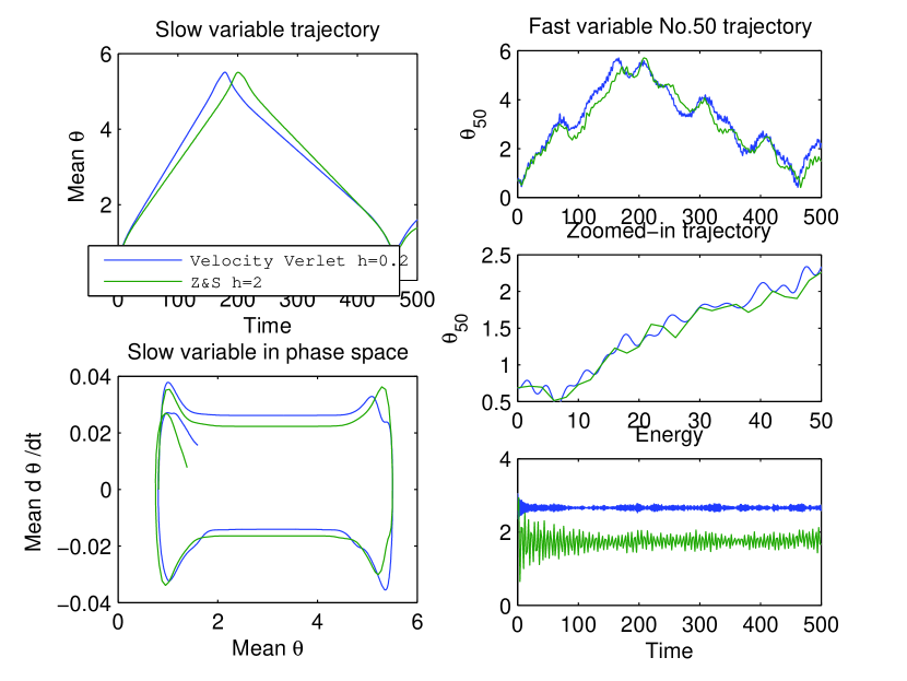
Figure 8: DNA ($N=200$ base-pairs) conformational transitions by Z&S and Velocity-Verlet.

It is known [63] that $\bar{\theta}=\sum\theta_{k}/N$ is a slow variable and can be used as a reaction parameter, whereas individual $\theta_{k}$’s are fast variables. Figure 8 presents simulations by Velocity-Verlet (benchmark) and Z&S ($\beta=0.3$) in these variables. The phase portrait shows that the DNA transits between meta-stable configurations $\theta=\text{arccos}(0.7)\approx 0.795$ and $\theta=2\pi-\text{arccos}(0.7)\approx 5.49$. Note these are long time simulations and the system is chaotic [43].

The Z&S energy is lower than the benchmark because fast oscillations are damped by large time-steps. Both $h=0.2$ in Velocity-Verlet and $h=2$ in Z&S are near stability limits. The methods respectively used 23.26 and 3.24 seconds CPU time.

4.5 Lie group integration

Formulating Z&S as a variational principle allows us to generalize the method to mechanical systems on Lie groups.

Consider a prototypical example of magnetized 3D rigid body with identity inertia matrix immersed in a constant magnetic field. The configuration space is $Q=\text{SO}(3)$. Denote by $R(t)\in Q$ the (generalized) rigid body position; in coordinates it is a $3\times 3$ matrix satisfying $R^{T}R=I$. Suppose when $R=I$ both the magnetic field and the dipole are in $z$-direction, then the potential energy can be written as $V(R)=\langle\mu Re_{3},Be_{3}\rangle=B\mu e_{3}^{T}R^{-1}e_{3}$, where $B$ and $\mu$ are field strength and dipole moment, and $e_{3}=\begin{bmatrix}0&0&1\end{bmatrix}^{T}$.

Let $\Omega(t)\in\mathbb{R}^{3}$ be convective angular velocity of the body, then the kinetic energy is $\frac{1}{2}\Omega^{T}\Omega$. Introduce an isomorphism between $\mathbb{R}^{3}$ and $\mathfrak{so}(3)$ (the Lie algebra of $\text{SO}(3)$) by

$$\Omega\mapsto\hat{\Omega}=\begin{bmatrix}0&-\Omega_{3}&\Omega_{2}\\ \Omega_{3}&0&-\Omega_{1}\\ -\Omega_{2}&\Omega_{1}&0\end{bmatrix}.$$

Then $\dot{R}=R\hat{\Omega}$. It is known [40] that dynamics of this mechanical system can be obtained from either of the following equivalent variational principles:

• $$\delta\int_{0}^{T}L(R,\dot{R})dt=0,$$ (32)

  with arbitrary variations of $R(t)\in Q$.

• $$\delta\int_{0}^{T}l(R,\xi)dt=0,$$ (33)

  with variations in the form $\delta\xi=\dot{\eta}+\text{ad}_{\xi}\eta$ under $R\in Q$ and $\xi=R^{-1}\dot{R}$.

For our system, $L(R,\dot{R})=\frac{1}{4}\text{tr}(\dot{R}^{T}\dot{R})-B\mu e_{3}^{T}R^{-1}e_{3}$ and $l(R,\hat{\Omega})=\frac{1}{2}\Omega^{T}\Omega-B\mu e_{3}^{T}R^{-1}e_{3}$ (note $\Omega^{T}\Omega=\frac{1}{2}\text{tr}(\hat{\Omega}^{T}\hat{\Omega})$).

We propose to simulate the system by modifying (32). The result is compared to a benchmark derived from (33) via Hamilton-Pontryagin princple, backward Variational Euler discretization, and Cayley approximation of the exponential map (see [25, 18] for Cayley approximation, [8] for the benchmark method, and [26, 36] for examples of other Lie group integrators). The benchmark uses update rules:

$$\begin{cases}R_{k+1}&=R_{k}\left(I-h\hat{\Omega}_{k+1}/2\right)^{-1}\left(I+h\hat{\Omega}_{k+1}/2\right)\\ \hat{\Omega}_{k+1}&=\hat{\Omega}_{k}+\frac{h^{2}}{4}\left(\hat{\Omega}_{k+1}^{T}\hat{\Omega}_{k+1}\hat{\Omega}_{k+1}^{T}-\hat{\Omega}_{k}^{T}\hat{\Omega}_{k}\hat{\Omega}_{k}^{T}\right)+hR_{k}\frac{\partial l}{\partial R}(R_{k},\hat{\Omega}_{k+1}).\end{cases}$$ (34)

Note $R$ is in a 3-dimensional manifold, and the differential in the last term shouldn’t be computed as partial derivative with respect to 9 Cartesian coordinates of $R$, otherwise the last term won’t be in $\mathfrak{so}(3)$. Instead, we follow [23] and obtain

$$hR_{k}\frac{\partial l}{\partial R}(R_{k},\hat{\Omega}_{k+1})=hB\mu R_{k}\frac{-e_{3}^{T}R_{k}^{-1}e_{3}}{\partial R_{k}}=hB\mu{\left((R_{k}^{-1}e_{3})\times e_{3}\right)}^{\wedge}.$$ (35)

(34) is variational and thus numerically energy and momentum preserving. Thanks to Cayley approximation, it also preserves the SO(3) structure in the sense that $R_{k}^{T}R_{k}=I$ up to arithmetic error. However, variational methods of this type are intrinsically nonlinearly implicit due to curved geometry when $Q$ is noncommutative (e.g., [8, 32]).

Our goal is to avoid expensive nonlinear solves and bypass force evaluations that require geometric calculations (such as (35)). To do so, we first add penalization to (32):

$$\delta\int_{0}^{T}\frac{1}{4}\text{tr}(\dot{R}^{T}\dot{R})-B\mu R(3,3)+\frac{1}{2}\omega^{2}\text{tr}((R^{T}R-I)^{T}(R^{T}R-I))dt=0,$$

where $R\in\text{SO}(3)$ is relaxed to $R\in\mathbb{R}^{3\times 3}$. We then discretize the action as follows:

$$\mathcal{L}_{d}(R_{k},R_{k+1},a_{k})=\text{tr}\left(\frac{1}{4}\left(\frac{R_{k+1}-R_{k}}{h}\right)^{T}\left(\frac{R_{k+1}-R_{k}}{h}\right)-\beta h^{2}\frac{1}{2}a_{k}^{T}a_{k}\right)$$

$$\qquad-B\mu e_{3}^{T}(R_{k}+\beta h^{2}a_{k})e_{3}-\text{tr}\left(\frac{1}{2}\omega^{2}\left(\left((R_{k}+\beta h^{2}a_{k})^{T}(R_{k}+\beta h^{2}a_{k})-I\right)^{2}\right)\right)$$ (36)

Finally, we truncate terms that are higher than 2nd-order in $a_{k}$. After using trace identities $\text{tr}(AB)=\text{tr}(BA)$ and $\text{tr}(A^{T})=\text{tr}(A)$, the truncated action simplifies to

$$\tilde{\mathcal{L}}_{d}(R_{k},R_{k+1},a_{k})=\text{tr}\left(\frac{1}{4}\left(\frac{R_{k+1}-R_{k}}{h}\right)^{T}\left(\frac{R_{k+1}-R_{k}}{h}\right)-\beta h^{2}\frac{1}{2}a_{k}^{T}a_{k}\right)$$

$$\qquad-B\mu e_{3}^{T}(R_{k}+\beta h^{2}a_{k})e_{3}-\text{tr}\Bigg{(}\frac{1}{2}\omega^{2}\Big{(}(R_{k}^{T}R_{k}-I)^{2}+4\beta h^{2}(R_{k}^{T}R_{k}R_{k}^{T}-R_{k}^{T})a_{k}$$

$$\qquad\qquad\qquad\qquad+2\beta^{2}h^{4}(a_{k}^{T}a_{k}R_{k}^{T}R_{k}+R_{k}^{T}a_{k}R_{k}^{T}a_{k}+a_{k}^{T}R_{k}R_{k}^{T}a_{k}-a_{k}^{T}a_{k})\Big{)}\Bigg{)}.$$

Unconstrained variation of this action with respect to $a_{k}$ gives

$$a_{k}=-B\mu e_{3}e_{3}^{T}-2\omega^{2}\left(R_{k}R_{k}^{T}R_{k}-R_{k}+\beta h^{2}(a_{k}R_{k}^{T}R_{k}+R_{k}a_{k}^{T}R_{k}+R_{k}R_{k}^{T}a_{k}-a_{k})\right).$$ (37)

Standard variational integrator construction leads to

$$p_{k}=-D_{1}\tilde{\mathcal{L}}_{d}(R_{k},R_{k+1},a_{k}),\qquad p_{k+1}=D_{2}\tilde{\mathcal{L}}_{d}(R_{k},R_{k+1},a_{k}).$$

Let $f_{k}=a_{k}+2\omega^{2}\beta^{2}h^{4}\left(a_{k}^{T}a_{k}R_{k}^{T}+a_{k}^{T}R_{k}a_{k}^{T}+R_{k}^{T}a_{k}a_{k}^{T}\right)$ and use (37) for simplification, then the above becomes

$$\begin{cases}p_{k+1}&=p_{k}+hf_{k}\\ R_{k+1}&=R_{k}+2hp_{k+1}\end{cases}.$$

These are our variational linearized SO(3) integrator. Note (36) is based on a 1st-order quadrature; 2nd-order trapezoidal rule would lead to

$$\begin{cases}p_{k+1/2}&=p_{k}+\frac{h}{2}f_{k}\\ R_{k+1}&=R_{k}+2hp_{k+1}\\ p_{k+1}&=p_{k}+\frac{h}{2}f_{k+1}\end{cases}.$$

These are similar to Z&S updates (Integrator 3) although Z&S works in $\mathbb{R}^{n}$. Some may question the usefulness of a variational formulation, because one can vectorize $R$ into $9$-dimension, view the penalized system as Newton’s equation, and then use Z&S. In Z&S updates (3), however, $V^{(3)}$ is essentially a 6-tensor, and its brute-force calculation in coordinates, as well as its contractions with $a$ from both left and right, will be unpleasant. A variational approach minimizes the involvement of coordinates and reduces the effort.

Figure 9: Snapshots of magnetized rigid body dynamics. Red and black arrows represent magnetic field and dipole.

Figure 9 demonstrates benchmark ($h=0.0001$) and variational Z&S simulations ($h=0.1$, $\omega=10$, $\beta=0.4$); their difference, regarded as our method’s error, is quantified in Figure 10(a); error of the benchmark method with $h=0.1$ is also provided in Figure 10(b) as a comparison. The full simulation is available at http://youtu.be/29deMRDRsuU. Initial conditions are $R(0)=I$ and $\Omega(0)=[1;0.2;0.1]$.

Our method and variational Euler with both $h=0.1$ respectively spent 0.03 and 1.45 seconds on computations. However, variational Lie group integrator is much better at preserving the Lie group structure. Applicabilities of the two approaches are disjoint: for example, variational Z&S generally suits computer graphics better, where real time rendering requires high efficiency, while demand on accuracy is moderate (as long as the result looks good); to orient satellites (e.g., [29]), on the other hand, one should choose variational Lie group integrators over variational Z&S, and it is worth CPU hours to precompute trajectories with high fidelity.

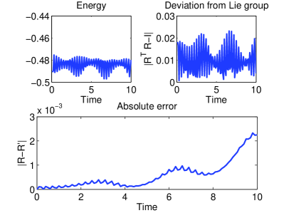
(a) Variational Z&S ($h=0.1$)

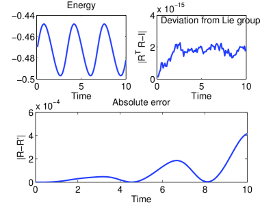
(b) Variational Euler on Lie group ($h=0.1$)

Figure 10: Preservation of energy, Lie group structure, and deviation from benchmark trajectory $R^{\prime}$.

5 Acknowledgement

This work was supported by NSF grant CMMI-092600, a generous gift from UTRC, and Courant Instructorship from New York University. We thank Mathieu Desbrun for motivation and discussions, Joel Tropp and Eitan Grinspun for discussions, Carmen Sirois for proofreading the manuscript, and anonymous reviewers for comments.

6 Appendix

Lemma 6.1.

Consider (7). If $V$ is bounded from below, then there is a constant $C$, such that $\|g(q^{\omega}(s))\|\leq C/\omega$ for all $s$. Moreover, if $V(q)$ diverges to infinity as $|q|\rightarrow\infty$, then there is a constant $\tilde{C}$ such that $\|q^{\omega}(s)\|\leq\tilde{C}$.

Proof.

Note the energy $[\dot{q}^{\omega}]^{T}M\dot{q}^{\omega}/2+V(q^{\omega})+\omega^{2}g(q^{\omega})^{T}g(q^{\omega})$ in the penalized system (7) is conserved and determined by initial condition. Therefore, $V(\cdot)$ being bounded from below and $g^{T}g\geq 0$ imply that $\omega^{2}g(q^{\omega})^{T}g(q^{\omega})=\mathcal{O}(1)$. Hence $g(q^{\omega}(s))=\mathcal{O}(1/\omega)$.

By a similar energy argument, since $[\dot{q}^{\omega}]^{T}M\dot{q}^{\omega}/2\geq 0$ and $g(q^{\omega})^{T}g(q^{\omega})\geq 0$, $V(q^{\omega})$ is bounded from above too, which implies that $q^{\omega}$ remains bounded. ∎

Lemma 6.2.

Consider the solution to a conserved mechanical system

$$\begin{cases}\ddot{x}^{\omega}=f_{1}(x^{\omega},y^{\omega})\\ \ddot{y}^{\omega}=f_{2}(x^{\omega},y^{\omega})-\omega^{2}g(y^{\omega})^{T}\nabla g(y^{\omega})\end{cases},$$ (38)

where $x^{\omega}$ and $y^{\omega}$ are vectors, and $x^{\omega}(0)=x_{0}$, $\dot{x}^{\omega}(0)=\dot{x}_{0}$, $y^{\omega}(0)=y_{0}$, $\dot{y}^{\omega}(0)=\dot{y}_{0}$. Suppose $f_{1}$, $f_{2}$ and $\nabla g$ are $C^{1}$ with bounded derivatives, $x^{\omega}$ and $y^{\omega}$ are bounded, $g(y_{0})=0$ and $\frac{d}{dt}g(y_{0})=0$, and $g(\cdot)$ has a non-degenerate Jacobian in a neighborhood of $y_{0}$, then

$$\lambda(t):=-\lim_{T\rightarrow 0}\lim_{\omega\rightarrow\infty}\frac{1}{T}\int_{t}^{t+T}\omega^{2}g(y^{\omega}(s))\,ds$$ (39)

exists and is finite. Denote by $x(t)$, $y(t)$ the solution to

$$\begin{cases}\ddot{x}=f_{1}(x,y)\\ \ddot{y}=f_{2}(x,y)+\lambda^{T}\nabla g(y)\\ g(y)=0\end{cases}$$ (40)

with the same initial conditions $x_{0},\dot{x}_{0},y_{0},\dot{y}_{0}$, then as $\omega\rightarrow\infty$,

$$\begin{cases}x^{\omega}\rightarrow x\\ y^{\omega}\xrightarrow{F}y\\ g(y^{\omega})\rightarrow 0\end{cases}$$ (41)

Proof.

We employ the multiscale averaging framework described in [61] to demonstrate the convergence. Here $x^{\omega}$ is a slow variable and its evolution corresponds to the constrained dynamics. $y^{\omega}$ is a fast variable corresponding to a fluctuating deviation from the constraint manifold at a characteristic timescale of $\mathcal{O}(1/\omega)$, and it lies in the normal bundle of the constraint manifold.

First, consider the linear constraint case in which $g(y)=Cy^{T}$ for some non-singular $C$ (the affine case can be similarly treated by shifting $y$). $y$ dynamics is governed by

$$\ddot{y}^{\omega}=f_{2}(x^{\omega},y^{\omega})-\omega^{2}y^{\omega}C^{T}C.$$ (42)

This is a forced harmonic oscillator, and its solution can be written as:

$$y^{\omega}(t)=\int_{0}^{t}f_{2}(x^{\omega}(s),y^{\omega}(s))\sin(\omega\tilde{C}s)\tilde{C}^{-1}/\omega\,ds,$$ (43)

where $\tilde{C}=\sqrt{C^{T}C}$ is the well-defined matrix square root, and matrix sin is defined either by Taylor expansion or diagonalization. Note there is no propagation of initial condition because $y^{\omega}(0)=0$.

It can be shown from (43) (for instance, by Lemma 3.8 in [60]; the idea is that an addition $1/\omega$ comes from the $\sin$ due to integration by parts) that $y^{\omega}(t)$ is $\mathcal{O}(\omega^{-2})$ at least up to $t=o(1)$, and $y^{\omega}$ is asymptotically periodic (because (42) is asymptotically linear) and hence locally ergodic on energy shell (with Dirac ergodic measure).

Since $y^{\omega}$ is locally ergodic on energy shell, (39) well-defines $\lambda$, and Theorem 1.2 in [61] guarantees that the effective equation for (42) is

$$\ddot{y}=f_{2}(x^{\omega},y)+\lambda^{T}C,$$ (44)

in the sense that $y^{\omega}\xrightarrow{F}y$ and $x^{\omega}\rightarrow x$. Notice that the convergence on $x$ is in the strong sense, i.e., $\lim_{\omega\rightarrow\infty}x^{\omega}(t)\rightarrow x(t)$ for all bounded $t>0$. This is because $x$ is purely slow, for which case, F-convergence implies strong convergence.

Now consider a fully nonlinear $g(\cdot)$ with a non-degenerate Jacobian. Lemma 6.1 gives that $g(y^{\omega})=\mathcal{O}(1/\omega)$. Since $y^{\omega}$ is by assumption bounded, inverting $g$ leads to $y^{\omega}-y_{0}=\mathcal{O}(1/\omega)$. Consequently, the dynamics of $y^{\omega}$ approaches that of a forced oscillator (with equilibrium at $y_{0}$) at a $\mathcal{O}(1/\omega)$ timescale, because $g(\cdot)$ is approximated by its first order Taylor expansion:

$$\ddot{y^{\omega}} =f_{2}(x^{\omega},y^{\omega})-\omega^{2}g(y^{\omega})^{T}\nabla g(y^{\omega})$$

$$=f_{2}(x^{\omega},y^{\omega})-\omega^{2}(\nabla g(y_{0})(y^{\omega}-y_{0})^{T}+\mathcal{O}(\omega^{-2}))^{T}(\nabla g(y_{0})+\text{Hess}\,g(y_{0})(y^{\omega}-y_{0})^{T}+\mathcal{O}(\omega^{-2}))$$

$$=f_{2}(x^{\omega},y^{\omega})-\omega^{2}(y^{\omega}-y_{0})\nabla g(y_{0})^{T}\nabla g(y_{0})+\mathcal{O}(1),$$

where nonlinearity $f_{2}+\mathcal{O}(1)$ again manifests as a slow force, which is dominated by the linear term that leads to asymptotically periodic oscillations. Hence, similar to the linear case, $y^{\omega}$ is locally ergodic on energy shell, the Lagrange multiplier $\lambda$ is well-defined, and the solution $x^{\omega}$, $y^{\omega}$ F-converges to the effective solution $x$, $y$. ∎

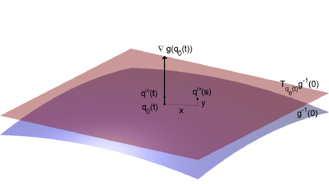
Figure 11: Multiscale geometry of penalized constrained dynamics – $x$ and $y$ are slow and fast.

Sketch of the proof of Theorem 11. (Figure 11 illustrates the notations used in the proof to help understand the geometry.) Since $g(q^{\omega})$ is at most $\mathcal{O}(1/\omega)$ (Lemma 6.1), $q^{\omega}$ is close to the constraint manifold $g^{-1}(0)$ in the sense that if we define for all $t$:

$$q_{0}(t):=\min_{q\in g^{-1}(0)}\|q-q^{\omega}(t)\|$$ (45)

then $q^{\omega}(t)-q_{0}(t)=\mathcal{O}(1/\omega)$. Indeed, given that $\nabla g$ has the maximum rank, $\nabla g(q_{0}(t))$ spans the normal section (i.e., the subspace perpendicular to the tangent subspace) of the constraint manifold, in which $q^{\omega}(t)-q_{0}(t)$ also lies. Moreover, $g$ restricted to each normal section is an isomorphism, and both the restricted map and its inverse have bounded norms due to the boundedness of $q^{\omega}$ (i.e., compactness of the solution space) — this is why $g(q^{\omega})=\mathcal{O}(1/\omega)$ implies $q^{\omega}(t)-q_{0}(t)=\mathcal{O}(1/\omega)$.

The idea is that since $q^{\omega}$ is close enough, the constraint manifold can be locally viewed as a flat subspace, and F-convergence for this case has been proved in Lemma 41. More precisely, there exists a linear isomorphism $A_{q_{0}(t)}$, such that

$$A_{q_{0}(t)}(q^{\omega}(t)-q_{0}(t))=\begin{bmatrix}0\\ y\end{bmatrix}$$ (46)

where $y$ is a vector with codimension of $g^{-1}(0)$ and $0$ is a null vector.

For $q^{\omega}(s)$ with $s-t=\mathcal{O}(1/\omega)$, we will have a full-dimensional representation:

$$A_{q_{0}(t)}(q^{\omega}(s)-q_{0}(t))=\begin{bmatrix}x\\ y\end{bmatrix},$$ (47)

and $x$ and $y$ will respectively be the slow and fast variables, representing the constrained dynamics and fluctuations away from the constraint manifold (analogous to Lemma 41). This is because

$$\frac{d^{2}}{ds^{2}}\begin{bmatrix}x\\ y\end{bmatrix} =A_{q_{0}(t)}(-\nabla V(q^{\omega}(s))-\omega^{2}g(q^{\omega}(s))\nabla g(q^{\omega}(s)))$$

$$=\begin{bmatrix}f_{1}(x,y)\\ f_{2}(x,y)\end{bmatrix}+\begin{bmatrix}\mathcal{O}(1)\\ -\omega^{2}\tilde{g}(y)\nabla\tilde{g}(y)+\mathcal{O}(1)\end{bmatrix},$$ (48)

where $f_{1}$ and $f_{2}$ are defined as $A_{q_{0}(t)}(-\nabla V(q^{\omega}(s))$. The $\mathcal{O}(1)$ in the 1st row of the right hand side of (48) is because $A_{q_{0}(t)}$ rotates the normal section to the y-direction, i.e.,

$$A_{q_{0}(t)}\nabla g(q^{\omega}(s))=A_{q_{0}(t)}(\nabla g(q_{0})+\mathcal{O}(1/\omega))=\begin{bmatrix}0\\ *\end{bmatrix}+\mathcal{O}(1/\omega),$$ (49)

where $*$ is some non-zero expression, and certainly $\mathcal{O}(1/\omega)=\mathcal{O}(1)$.

The $\mathcal{O}(1)$ in the 2nd row of the right hand side of (48) can also be intuitively obtained by using an analogous geometric argument, together with Taylor expansion.

Since (48) corresponds to the locally flat system (38), Lemma (41) proved the existence of an equivalent Lagrange multiplier as well as the F-convergence towards it. Moreover, (48) and the global dynamics near the curved constraint manifold (7) is linked via a coordinate transformation $q^{\omega}\mapsto A_{q_{0}}(q^{\omega}-q_{0})$, which, naturally, is slowly varying as $q_{0}$ changes. Since averaging via F-convergence (Theorem 1.2 in [61]) still works if the slow and fast variables are images of the original variable under a slowly varying diffeomorphism, the global dynamics (7) is F-convergent to a solution of (9). Notice that $g(q(t))=0$ in (9) is automatically satisfied, because $\lim_{\omega\rightarrow\infty}g(q^{\omega}(t))=0$.

Finally, the solution to (9) is also the solution to (6). This is by the existence and uniqueness of the solution to differential algebraic equations with initial conditions.

(Only main lines of the proof are provided; details are similar to analysis in [61, 60]). $\blacksquare$

Remark 6.1.

The above proofs show that $g(q^{\omega}(s))$ is not only $\mathcal{O}(\omega^{-1})$ but $\mathcal{O}(\omega^{-2})$.

References

- [1] R. Abraham and J. E. Marsden, Foundations of Mechanics, American Mathematical Society, 2nd ed., 2008.
- [2] H. C. Andersen, Rattle: A “velocity” version of the shake algorithm for molecular dynamics calculations, J. Comput. Phys, 52 (1983), pp. 24–34.
- [3] J. Bajars, J. Frank, and B. Leimkuhler, Stochastic-dynamical thermostats for constraints and stiff restraints, The European Physical Journal Special Topics, 200 (2011), pp. 131–152.
- [4] R. M. Beam and R. Warming, An implicit finite-difference algorithm for hyperbolic systems in conservation-law form, Journal of Computational Physics, 22 (1976), pp. 87 – 110.
- [5] F. Bornemann, Homogenization in time of singularly perturbed mechanical systems, vol. 1687 of Lecture Notes in Mathematics, Springer, Berlin, Heidelberg, New York, 1998.
- [6] F. A. Bornemann and C. Schütte, A mathematical approach to smoothed molecular dynamics: Correcting potentials for freezing bond angles, Konrad-Zuse-Zentrum für Informationstechnik Berlin, 1995.
- [7] , Homogenization of hamiltonian systems with a strong constraining potential, Physica D: Nonlinear Phenomena, 102 (1997), pp. 57–77.
- [8] N. Bou-Rabee and J. E. Marsden, Hamilton–Pontryagin integrators on Lie groups part I: Introduction and structure-preserving properties, Foundations of Computational Mathematics, 9 (2009), pp. 197–219.
- [9] N. Bou-Rabee and H. Owhadi, Long-run accuracy of variational integrators in the stochastic context, SIAM J. Numer. Anal., 48 (2010), pp. 278–297.
- [10] P. J. Channell and C. Scovel, Symplectic integration of hamiltonian systems, Nonlinearity, 3 (1990), p. 231.
- [11] F. Chiba and T. Kako, Newmark’s method and discrete energy applied to resistive mhd equation, Vietnam J. Math., 30 (2002), pp. 501–520.
- [12] S. Erlicher, L. Bonaventura, and O. S. Bursi, The analysis of the Generalized method for non-linear dynamic problems, Comput. Mech., 28 (2002), pp. 83–104.
- [13] E. Faou and B. Grebert, Hamiltonian interpolation of splitting approximations for nonlinear PDEs, Foundations of Computational Mathematics, 11 (2011), pp. 381–415.
- [14] F. Filbet and S. Jin, A class of asymptotic preserving schemes for kinetic equations and related problems with stiff sources, (2010). arXiv:0905.1378. Accepted by J. Comput. Phys.
- [15] M. Fixman, Classical statistical mechanics of constraints: A theorem and application to polymers, Proc. Nat. Acad. Sci. USA, 71-8 (1974), pp. 3050–3053.
- [16] B. García-Archilla, J. M. Sanz-Serna, and R. D. Skeel, Long-time-step methods for oscillatory differential equations, SIAM J. Sci. Comput., 20 (1999), pp. 930–963.
- [17] L. F. Greengard and V. Rokhlin, A fast algorithm for particle simulations, J. Comput. Phys, 73 (1987), pp. 325–348.
- [18] E. Hairer, C. Lubich, and G. Wanner, Geometric Numerical Integration: Structure-Preserving Algorithms for Ordinary Differential Equations, Springer, Berlin Heidelberg New York, second ed., 2006.
- [19] E. Hairer and G. Wanner, Solving ordinary differential equations II, Springer, 2nd ed., 1996.
- [20] C. Hartmann, An ergodic sampling scheme for constrained hamiltonian systems with applications to molecular dynamics, Journal of Statistical Physics, 130 (2008), pp. 687–711.
- [21] B. Hess, H. Bekker, H. J. C. Berendsen, and J. G. E. M. Fraaije, LINCS: A linear constraint solver for molecular simulations, J. Comput. Chem., 18 (1997), pp. 1463–1472.
- [22] J. S. Hesthaven, S. Gottlieb, and D. Gottlieb, Spectral Methods for Time-Dependent Problems, vol. 21 of Cambridge Monographs on Applied and Computational Mathematics, Cambridge University Press, United Kingdom, 2007.
- [23] D. D. Holm, J. E. Marsden, and T. S. Ratiu, The euler–poincaré equations and semidirect products with applications to continuum theories, Advances in Mathematics, 137 (1998), pp. 1–81.
- [24] T. J. R. Hughes, A note on the stability of newmark’s algorithm in nonlinear structural dynamics, Int. J. Numer. Meth. Eng., 11 (1977), pp. 383–386.
- [25] A. Iserles, On Cayley-transform methods for the discretization of Lie-group equations, Found. Comput. Math., 1 (2001), pp. 129–160.
- [26] A. Iserles, H. Z. Munthe-Kaas, S. P. Nørsett, and A. Zanna, Lie-group methods, Acta Numerica 2000, 9 (2000), pp. 215–365.
- [27] A. Jain, N. Vaidehi, and G. Rodriguez, A fast recursive algorithm for molecular dynamics simulation, J. Comput. Phys, 106 (1993), pp. 258–268.
- [28] W. L. Jorgensen, J. Chandrasekhar, J. D. Madura, R. W. Impey, and M. L. Klein, Comparison of simple potential functions for simulating liquid water, J. Chem. Phys., 79 (1983), p. 926.
- [29] O. Junge and S. Ober-Blobaum, Optimal reconfiguration of formation flying satellites, in Decision and Control, 2005 and 2005 European Control Conference. CDC-ECC’05. 44th IEEE Conference on, IEEE, 2005, pp. 66–71.
- [30] C. Kane, J. E. Marsden, M. Ortiz, and M. West, Variational integrators and the Newmark algorithm for conservative and dissipative mechanical systems, Int. J. Numer. Meth. Eng., 49 (2000), pp. 1295–1325.
- [31] J. Kevorkian and J. D. Cole, Multiple scale and singular perturbation methods, vol. 114 of Applied Mathematical Sciences, Springer-Verlag, New York, 1996.
- [32] M. Kobilarov, K. Crane, and M. Desbrun, Lie group integrators for animation and control of vehicles, ACM Transactions on Graphics, 28 (2009), p. 16.
- [33] W. Koon, H. Owhadi, M. Tao, and T. Yanao, Control of a model of DNA division via parametric resonance. arXiv:1211.4064. Submitted, 2012.
- [34] V. Kräutler, W. F. van Gunsteren, and P. H. H nenberger, A fast SHAKE algorithm to solve distance constraint equations for small molecules in molecular dynamics simulations, J. Comput. Chem., 22 (2001), pp. 501–508.
- [35] D. Kuhl and E. Ramm, Constraint energy momentum algorithm and its application to non-linear dynamics of shells, Computer Methods in Applied Mechanics and Engineering, 136 (1996), pp. 293 – 315.
- [36] T. Lee, M. Leok, and N. H. McClamroch, Lie group variational integrators for the full body problem, Computer Methods in Applied Mechanics and Engineering, 196 (2007), pp. 2907–2924.
- [37] B. Leimkuhler and S. Reich, Simulating Hamiltonian dynamics, vol. 14 of Cambridge Monographs on Applied and Computational Mathematics, Cambridge University Press, Cambridge, 2004.
- [38] T. Lelièvre, M. Rousset, and G. Stoltz, Langevin dynamics with constraints and computation of free energy differences, Mathematics of Computation, 81 (2012), pp. 2071–2125.
- [39] T. Li, A. Abdulle, and W. E, Effectiveness of implicit methods for stiff stochastic differential equations, Commun. Comput. Phys., 3 (2008), pp. 295–307.
- [40] J. E. Marsden and T. S. Ratiu, Introduction to Mechanics and Symmetry, Springer, 2nd ed., 2010.
- [41] J. E. Marsden and M. West, Discrete mechanics and variational integrators, Acta Numerica, (2001), pp. 357–514.
- [42] R. I. McLachlan and P. Atela, The accuracy of symplectic integrators, Nonlinearity, 5 (1992), p. 541.
- [43] I. Mezić, On the dynamics of molecular conformation, Proc. Natl. Acad. Sci., 103 (2006), pp. 7542–7547.
- [44] S. Miyamoto and P. A. Kollman, Settle: An analytical version of the SHAKE and RATTLE algorithm for rigid water models, J. Comput. Chem., 13 (1992), pp. 952–962.
- [45] F. Neri, Lie algebras and canonical integration, tech. report, Department of Physics, University of Maryland, 1988.
- [46] N. M. Newmark, A method of computation for structural dynamics, Proc. ASCE, 85 (1959), pp. 67–94.
- [47] D. Perchak, J. Skolnick, and R. Yaris, Dynamics of rigid and flexible constraints for polymers. Effect of the Fixman potential, Macromolecules, 18 (1985), pp. 519–525.
- [48] J. C. Platt and A. H. Barr, Constraints methods for flexible models, SIGGRAPH Comput. Graph., 22 (1988), pp. 279–288.
- [49] S. Reich, Smoothed dynamics of highly oscillatory Hamiltonian systems, Physica D: Nonlinear Phenomena, 89 (1995), pp. 28–42.
- [50] P. H. Richter and H.-J. Scholz, Stochastic phenomena and chaotic behaviour in complex systems, Springer-Verlag, Berlin and New York, 1984.
- [51] H. Rubin and P. Ungar, Motion under a strong constraining force, Communications on Pure and Applied Mathematics, 10 (1957), pp. 65–87.
- [52] J.-P. Ryckaert, G. Ciccotti, and H. J. C. Berendsen, Numerical integration of the cartesian equations of motion of a system with constraints: molecular dynamics of n-alkanes, J. Comput. Phys, 23 (1977), pp. 327–341.
- [53] J. M. Sanz-Serna, Mollified impulse methods for highly oscillatory differential equations, SIAM J. Numer. Anal., 46 (2) (2008), pp. 1040–1059.
- [54] T. Schlick, Molecular Modeling and Simulation, Springer, 2nd ed., 2010.
- [55] C. Schütte and F. A. Bornemann, Homogenization approach to smoothed molecular dynamics, Nonlinear analysis, theory, methods & applications, 30 (1997), pp. 1805–1814.
- [56] J. Shatah and C. Zeng, Periodic solutions for Hamiltonian systems under strong constraining forces, Journal of Differential Equations, 186 (2002), pp. 572–585.
- [57] R. D. Skeel and K. Srinivas, Nonlinear stability analysis of area-preserving integrators, SIAM J. Numer. Anal., 38 (2000), pp. 129–148.
- [58] R. D. Skeel, G. Zhang, and T. Schlick, A family of symplectic integrators: Stability, accuracy, and molecular dynamics applications, SIAM J. Sci. Comput., 18 (1997), pp. 203–222.
- [59] F. Takens, Motion under the influence of a strong constraining force, in Global theory of dynamical systems, Springer, 1980, pp. 425–445.
- [60] M. Tao, H. Owhadi, and J. E. Marsden, From efficient symplectic exponentiation of matrices to symplectic integration of high-dimensional Hamiltonian systems with slowly varying quadratic stiff potentials, Appl. Math. Res. Express, 2011, pp. 242–280.
- [61] , Nonintrusive and structure preserving multiscale integration of stiff ODEs, SDEs and Hamiltonian systems with hidden slow dynamics via flow averaging, Multiscale Model. Simul., 8 (2010), pp. 1269–1324.
- [62] D. Terzopoulos, J. Platt, A. Barr, and K. Fleischer, Elastically deformable models, SIGGRAPH Comput. Graph., 21 (1987), pp. 205–214.
- [63] P. D. Toit, I. Mezić, and J. Marsden, Coupled oscillator models with no scale separation, Phys. D, 238 (2009), pp. 490–501.
- [64] D. van der Spoel, P. J. van Maaren, and H. J. C. Berendsen, A systematic study of water models for molecular simulation: Derivation of water models optimized for use with a reaction field, J. Chem. Phys., 108 (1998), p. 10220.
- [65] E. Vanden-Eijnden and G. Ciccotti, Second-order integrators for Langevin equations with holonomic constraints, Chem. Phys. Lett., 429 (2006), pp. 310–316.
- [66] J. M. Wendlandt and J. E. Marsden, Mechanical integrators derived from a discrete variational principle, Phys. D, 106 (1997), pp. 223–246.
- [67] A. Witkin, K. Fleischer, and A. Barr, Energy constraints on parameterized models, SIGGRAPH Comput. Graph., 21 (1987), pp. 225–232.
- [68] W. L. Wood and M. E. Oduor, Stability properties of some algorithms for the solution of nonlinear dynamic vibration equations, Commun. Appl. Numer. Methods, 4 (1988), pp. 205–212.
- [69] H. Yoshida, Construction of higher order symplectic integrators, Phys. Lett. A, 150 (1990), pp. 262–268.
- [70] M. Zhang and R. D. Skeel, Cheap implicit symplectic integrators, Applied Numerical Mathematics, 25 (1997), pp. 297–302.