A Simple Parallelization Scheme for Extensive Air Shower Simulations

Abstract

A simple method for the parallelization of extensive air shower simulations is described. A shower is simulated at fixed steps in altitude. At each step, daughter particles below a specified energy threshold are siphoned off and tabulated for further simulation. Once the entire shower has been tabulated, the resulting list of particles is concatenated and divided into separate list files where each possesses a similar projected computation time. These lists are then placed on a computation cluster where the simulation can be completed in a piecemeal fashion as computing resources become available. Once the simulation is complete, the outputs are reassembled as a complete air shower simulation. The original simulation program (in this case CORSIKA) is in no way altered for this procedure. Verification is obtained by comparisons of $10^{16.5}$ eV showers produced with and without parallelization.

1 Introduction

In the past 50 years, much progress has been made in the understanding of Extensive Air Showers (EAS) associated with Ultra-High Energy Cosmic Rays (UHECRs). However, the historical difference in energy determination between Surface Detection (SD) [1][2][3][4] and Fluorescence Detection (FD) [5][6][7] has yet to be resolved. In its hybrid mode, the Pierre Auger experiment [8] reports a 30% discrepancy for simulation based energy determination between SD and FD for events observed in hybrid operation mode [9].

We posit that this discrepancy could be better understood if it were not for the fact that it has been computationally infeasible to simulate large numbers of EAS with primary energy $>10^{18}$ eV without utilizing statistical thinning methods that fully simulate only a small representative fraction of the EAS. These thinned simulations certainly can be adequate for calculating longitudinal profiles [10] and average lateral distributions [11]. However, they neither capture the full breadth of fluctuations at the distance scale of individual surface detector counters nor do they provide all of the specific particle information necessary to properly estimate counter energy deposition and the consequent electronic response.

Non-thinned simulations of UHECRs are very computationally intensive. Using a single modern CPU core, the simulation of the EAS for a single $10^{17}$ eV proton requires on the order of $1$ day. Simulation times increase more or less linearly with energy. Extrapolated to the logical extreme, this implies that, without continued progress in computational ability, the simulation of the largest UHECR observation reported thus far ($3.2\times 10^{20}$ eV [5]) could span the better part of a decade.

One solution for this computational deficiency is parallelization. By dividing the task between many different CPU cores, a simulation that previously would have taken years to conclude can be completed in days or even hours. By employing scoring strategies to optimize the division of labor, it is possible to simulate even the largest observed EAS with nothing more than the spare computational power that inadvertently arises in the scheduling of large jobs on computational clusters.

This paper is the first of three to describe methods used in the Telescope Array (TA) Collaboration [12, 13] to simulate EAS as seen by the TA surface detector (TASD). The second paper will deal with “dethinning,” that is, replacing the shower particles eliminated in the thinning process. The third paper will describe the simulation of the TASD response to EAS and show comparisons between the actual TASD data and a spectral set of simulated EAS.

2 Parallelization Overview

Simulation programs for EAS are particularly well-suited for parallelization because they do not contain self-interaction. That is, the individual daughter particles in the shower interact exclusively with atmospheric medium and not with each other. Thus, each EAS can be thought of as the superposition of many smaller sub-showers. Parallelization can then be carried out in the following steps:

1. Initially, a single computer is utilized to separate the EAS simulation into many smaller, more manageable, simulations by running the simulation repeatedly through small steps in atmospheric depth.

2. At each step, the simulation output is sorted with particles above a nominal upper threshold being passed back through the simulation. Particles below a lower variable threshold are discarded and the rest of the output is appended to a master list.

3. Eventually, all of the simulated particles fall below the nominal upper threshold. The master list contains all the input parameter sets necessary for a series of simulations that can be superimposed to reconstitute the the original EAS.

4. The master list is then divided into sub-lists and divided amongst a larger number of computers either manually or via clustering.

5. When all of the sub-list simulations are finished, the final total simulation can then be reassembled.

A critical aspect of this procedure is that the actual simulation source code is in no way altered. All aspects of parallelization are achieved by translating each generation of simulation output files into the next generation of simulation input files via a series of scripts and compiled programs under the direction of a master script which explicitly tracks spatial and temporal information for each component simulation.

3 Parallelization Application

While this is, in principle, a fairly straightforward procedure, it is important to consider how this procedure works in practice for a particular simulation package. For this purpose, we use CORSIKA v6.960 [14]. High energy hadronic interactions are modeled by QGSJET-II-03 [15], low energy hadronic interactions are modeled by FLUKA2008.3c [16, 17], and electromagnetic interactions are modeled by EGS4 [18].

As a first step, a CORSIKA “input card” is created for the primary particle. While this input card can encompass a wide range of CORSIKA options, there are some important constraints:

1. There is only one EAS in the simulation run.

2. The starting point of the arrival time scale is set to the first interaction. This greatly simplifies tracking time offsets later in the procedure

3. The zenith angle of the primary particle does not exceed $60^{\circ}$. This constraint is necessary in order to keep the primary zenith angles of the secondary EAS below $70^{\circ}$. Above $70^{\circ}$, CORSIKA uses a curved earth model which greatly complicates the propagation of temporal and spatial offsets through the parallelization.

4. The observation level is set high in the atmosphere (e.g. 80 km). By doing so, we minimize the simulation time for the linear stage of the procedure.

5. The ground level core location is set to have the same x-y coordinate system as the EAS.

Once an input card is created, it is submitted to the CORSIKA simulation package. The particles in the simulated output are then each assigned a score, $T_{i}$ which corresponds to the maximum time necessary to simulate a complete EAS down to the final observation level for that particle. The value of $T_{i}$ was determined using the following relation:

$$T_{i}\propto E_{i}\times e^{t_{si}/\tau},$$ (1)

where $E_{i}$ is the energy of the particle, $t_{si}$ is the atmosphere slant depth between the position of the particle and the ground, and $\tau=50$ g/cm². While this is a crude estimate of simulation time at best, it is fairly accurate insofar as the EAS maximum does not occur too far above the ground.

The particles are then divided into two categories: $T_{i}>T_{max}$ and $T_{i}<T_{max}$, where $T_{max}$ is the maximum time to completion for individual jobs in parallel portion of this process. Particles where $T_{i}<T_{max}$ are added to a master list. Each line of the list contains: $T_{i}$, particle type, energy, trajectory, position, time, and random number seeds.

For particles where $T_{i}>T_{max}$, the time and position are noted in a separate file and a new CORSIKA input card is generated. The new card has an observation level 50 g/cm² lower in slant depth than the starting altitude. The resulting set of input cards is then submitted to the CORSIKA package for simulation. The resulting particles have their times and positions offset by the initial values recorded above. This process undergoes many iterations until there are no particles where $T_{i}>T_{max}$.

Once the shower is decomposed into particles where $T_{i}<T_{max}$, a cut is applied on particles where $E_{i}<t_{vi}*(1$ MeV$\cdot$cm²/g) with $t_{vi}$ being the vertical depth between the particle and the ground level. This eliminates particles which are sufficiently low in energy that subsequent propagation would not be expected to persist to ground level due to either ionization and/or further EAS production. The resulting list of particles is then sorted into sub-lists where $\sum_{i}T_{i}\simeq T_{max}$.

The simulation can now be carried out in a parallel fashion. For each sub-list, CORSIKA input cards are created for each individual particle. This differs from the non-parallel portion above in that every EAS is simulated all the way to ground level. Once the EAS are simulated for every particle, the time and position offsets for each particle is applied to the respective CORSIKA output file and then all the EAS from the sub-list are concatenated into a single CORSIKA output file. From there, the final step is to further concatenate the concatenated sub-list outputs from the parallel jobs into a single CORSIKA output file.

The predominate advantage of this procedure lies in its inherent flexibility. Because each sub-list is independent in its execution, the simulation can proceed on whatever number of computational nodes is available and even on multiple systems. Because the size of each sub-list can be controlled by simply increasing or decreasing $T_{max}$ it is very simple to make use of whatever excess capacity might be available due to scheduling gaps in a large computational cluster. Furthermore, it would be trivial to adapt this method to volunteer computing.

4 Parallelization Validation

The parallelization method is validated by comparing pairs of EAS simulated with the same input parameters both with and without parallelization. For comparison purposes, we initiated with a $10^{16.5}$ eV proton at a fixed height of first interaction of 30 km. This comparatively low primary energy was chosen due to the time required to generate EAS without parallelization. Four different primary zenith angles were selected: $0^{\circ}$, $30^{\circ}$, $45^{\circ}$, and $60^{\circ}$. In Figures 1-4,

(a)

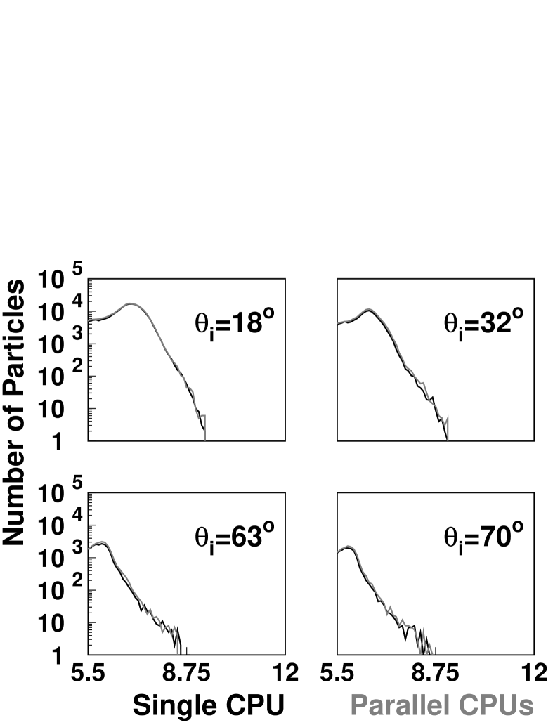
(b)

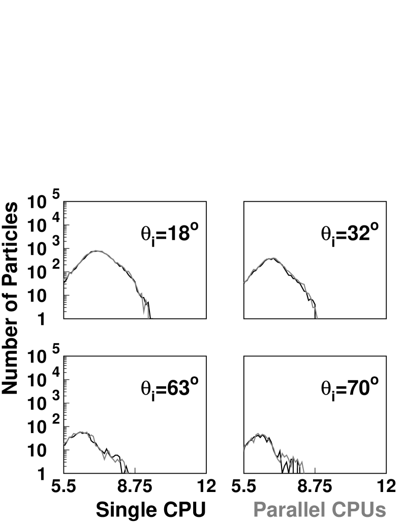
(c)

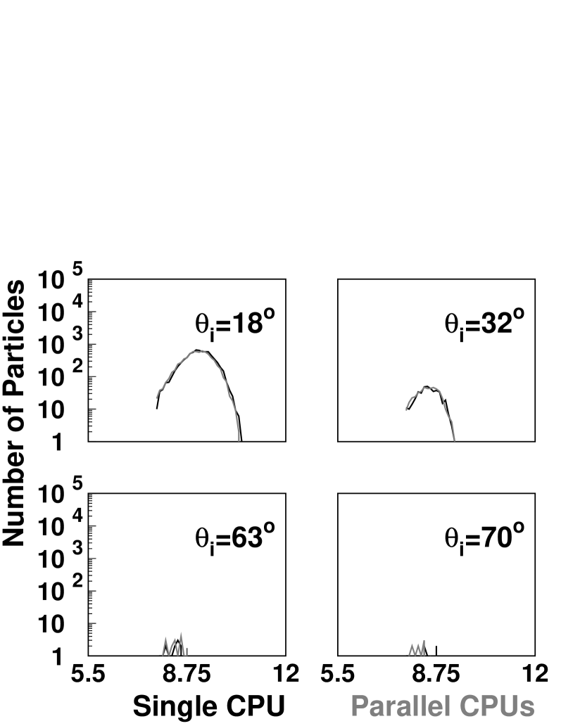
Figure 1: Comparison of secondary particle spectra for two protonic showers (one generated with a single CPU and one generated in parallel with many CPUs) with primary energy $E_{0}=10^{16.5}$ eV and primary zenith angle $\theta_{0}=0^{\circ}$. For each shower, simulated particles whose ground position was within a region enclosed by shower rotation angles $\Phi=[-30^{\circ},30^{\circ}]$ and lateral distances $r=[500{\rm m},1000{\rm m}]$ were tabulated with respect to particle type, incident angle with respect to the ground, $\theta_{i}$, and kinetic energy. The resulting spectra are shown in $\cos\theta_{i}=0.1$ increment bins for a) photons, b) electrons and positrons, and c) muons. For each histogram, good agreement is observed between simulations generated linearly (black) and via parallelization (gray).

(a)

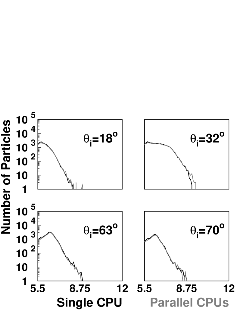
(b)

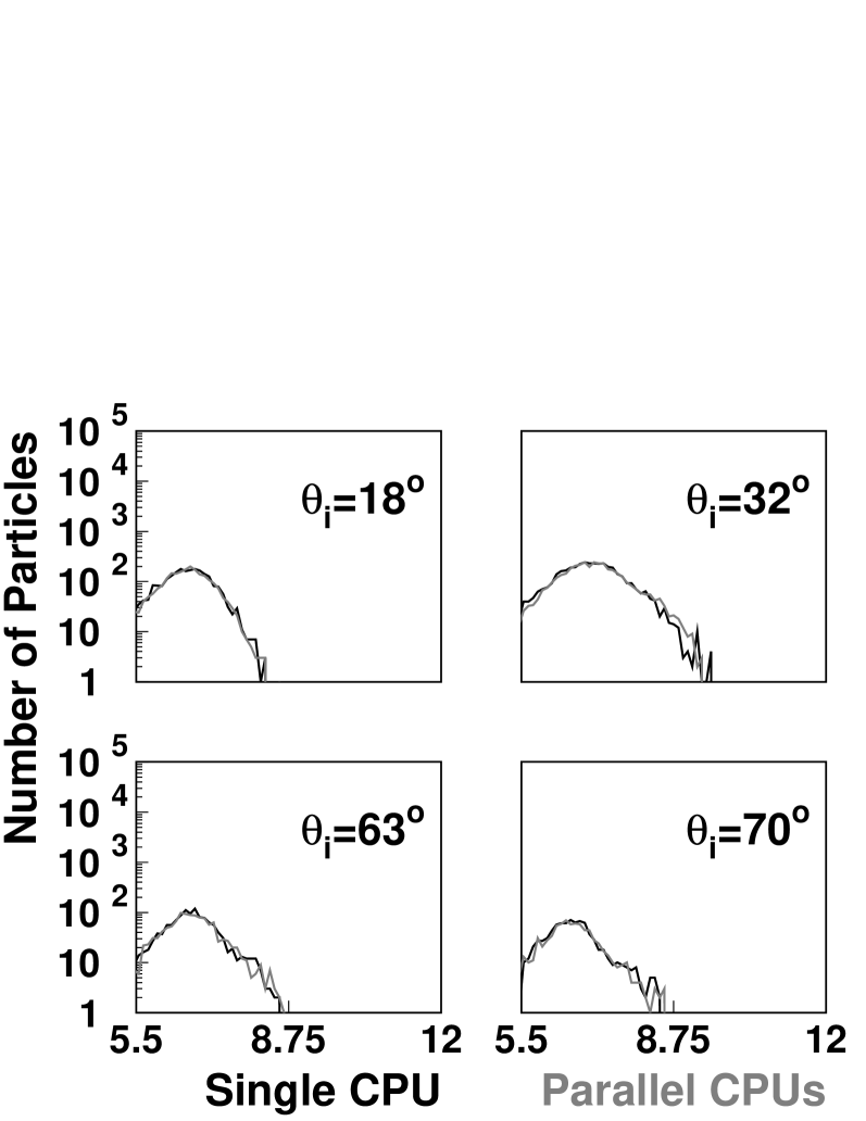
(c)

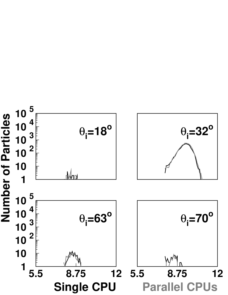
Figure 2: Comparison of secondary particle spectra for two protonic showers (one generated with a single CPU and one generated in parallel with many CPUs) with primary energy $E_{0}=10^{16.5}$ eV and primary zenith angle $\theta_{0}=30^{\circ}$. For each shower, simulated particles whose ground position was within a region enclosed by shower rotation angles $\Phi=[-30^{\circ},30^{\circ}]$ and lateral distances $r=[500{\rm m},1000{\rm m}]$ were tabulated with respect to particle type, incident angle with respect to the ground, $\theta_{i}$, and kinetic energy. The resulting spectra are shown in $\cos\theta_{i}=0.1$ increment bins for a) photons, b) electrons and positrons, and c) muons. For each histogram, good agreement is observed between simulations generated linearly (black) and via parallelization (gray).

(a)

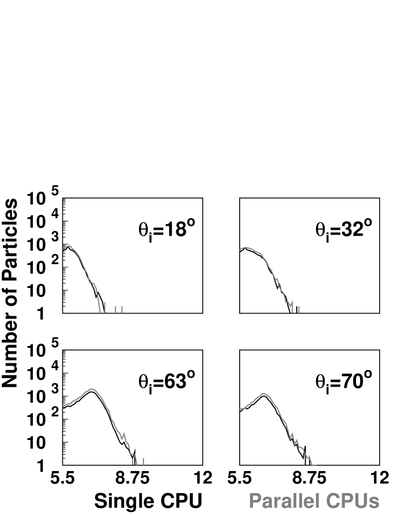
(b)

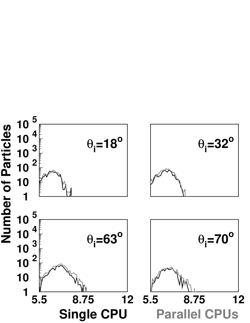
(c)

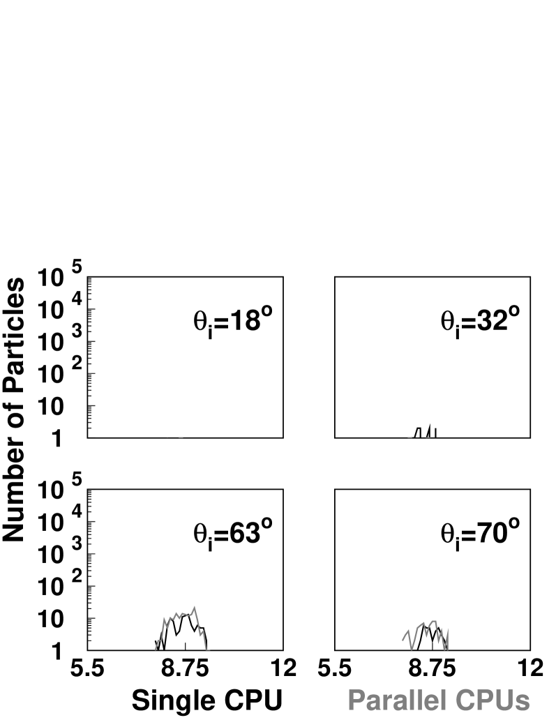
Figure 3: Comparison of secondary particle spectra for two protonic showers (one generated with a single CPU and one generated in parallel with many CPUs) with primary energy $E_{0}=10^{16.5}$ eV and primary zenith angle $\theta_{0}=45^{\circ}$. For each shower, simulated particles whose ground position was within a region enclosed by shower rotation angles $\Phi=[-30^{\circ},30^{\circ}]$ and lateral distances $r=[500{\rm m},1000{\rm m}]$ were tabulated with respect to particle type, incident angle with respect to the ground, $\theta_{i}$, and kinetic energy. The resulting spectra are shown in $\cos\theta_{i}=0.1$ increment bins for a) photons, b) electrons and positrons, and c) muons. For each histogram, good agreement is observed between simulations generated linearly (black) and via parallelization (gray).

(a)

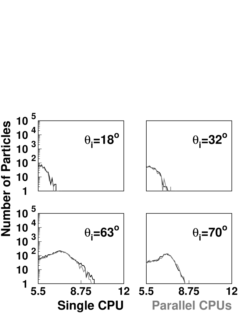
(b)

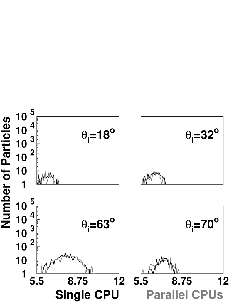
(c)

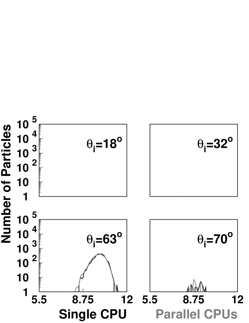
Figure 4: Comparison of secondary particle spectra for two protonic EAS simulations (one generated with a single CPU and one generated in parallel with many CPUs) with primary energy $E_{0}=10^{16.5}$ eV and primary zenith angle $\theta_{0}=60^{\circ}$. For each shower, simulated particles whose ground position was within a region enclosed by shower rotation angles $\Phi=[-30^{\circ},30^{\circ}]$ and lateral distances $r=[500{\rm m},1000{\rm m}]$ were tabulated with respect to particle type, incident angle with respect to the ground, $\theta_{i}$, and kinetic energy. The resulting spectra are shown in $\cos\theta_{i}=0.1$ increment bins for a) photons, b) electrons and positrons, and c) muons. For each histogram, good agreement is observed between simulations generated linearly (black) and via parallelization (gray).

we show comparisons of secondary spectra from CORSIKA EAS simulated with and without parallelization. While the same random number seeds were used for the single-process simulations and the top level of the parallelized simulations, this can only guarantee that the interactions down to the first observation level of the parallelization scheme (in this case 29 km) will be the same for the two simulations. Taking this built-in discrepancy into account, the simulations with and without parallelization agree remarkably well for Figures 1-4.

Another comparison that can be performed is to consider secondary particle arrival times for specific points at the ground observation level. For this purpose, we consider a ring in the plane normal to the EAS trajectory that intersects the ground at the shower core with a radius of 300 m and 2 m thickness. The ring is then further divided azimuthally into $\sim 1000$ 2-meter long segments. These segments are then projected onto the ground. For each segment, we tabulate the arrival time, $t_{0}$, of the first particle for each segment and the time, $t_{1/2}$, when 50% of the total particle flux for a given segment has arrived. These times are then corrected for the time offset between the positions of each segment on the ground and the plane normal to the EAS. In Figure 5,

(a)

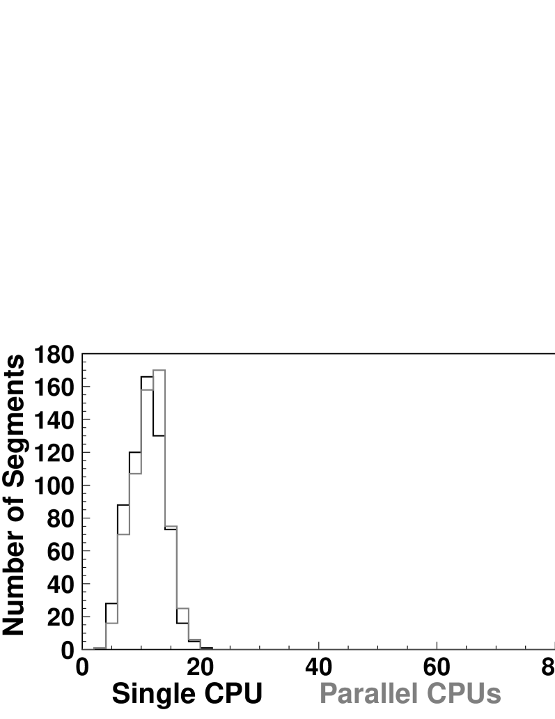
(b)

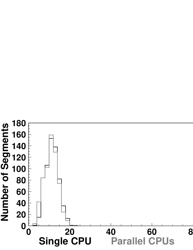
(c)

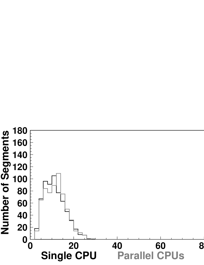
(d)

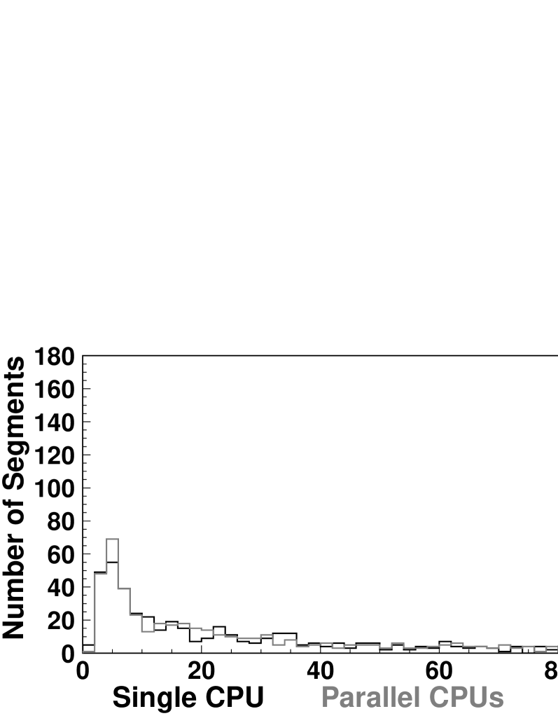
Figure 5: Comparison of distribution of initial arrival times, $t_{0}$, for $2\times 2$ m segments in plane normal to shower trajectory for $10^{16.5}$ eV protonic EAS simulations with primary zenith angles of a) $0^{\circ}$, b) $30^{\circ}$, c) $45^{\circ}$, and d) $60^{\circ}$. In each case, $t_{0}$ was measured for segments 200 m lateral distance from the shower core. For each histogram, good agreement in both mean value and variance are observed between simulations generated linearly (black) and via parallelization (gray).

we see comparative histograms of $t_{0}$ for all four simulation pairs described above. Figure 6

(a)

(b)

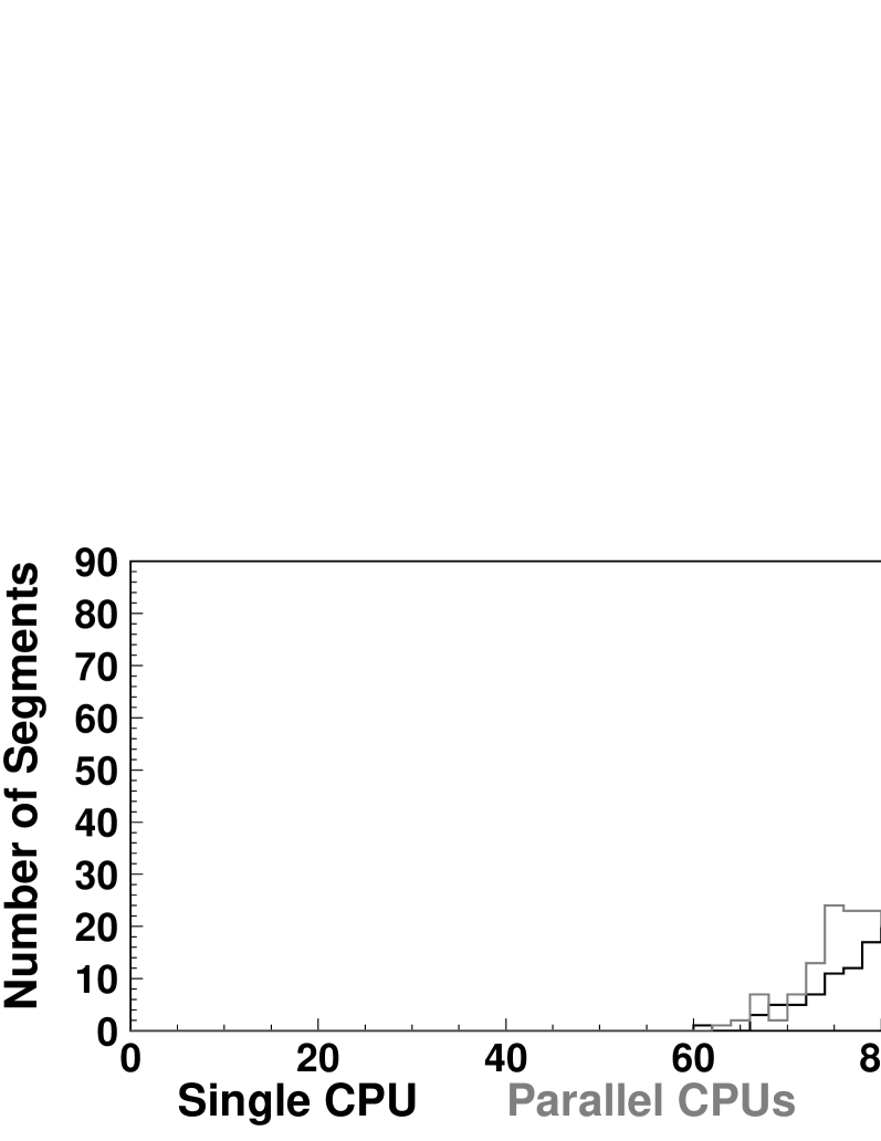
(c)

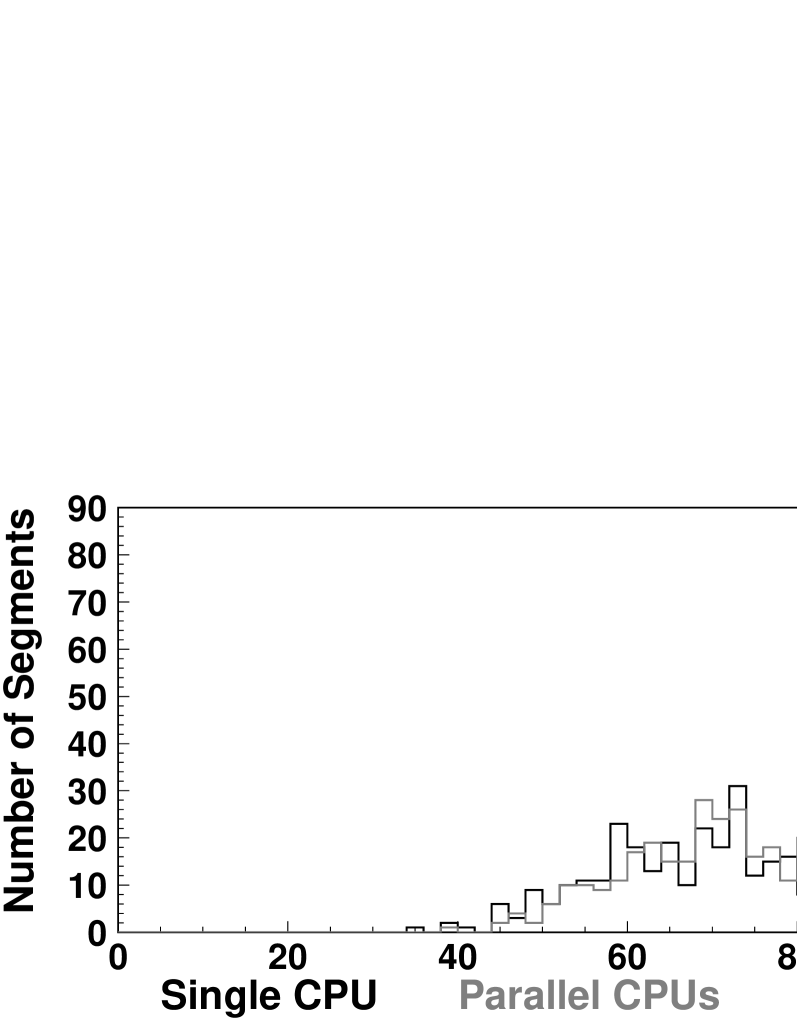
(d)

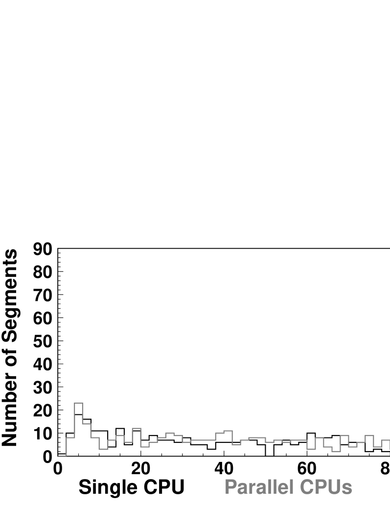
Figure 6: Comparison of distribution of median arrival times, $t_{1/2}$, for $2\times 2$ m segments in plane normal to shower trajectory for $10^{16.5}$ eV protonic EAS simulations with primary zenith angles of a) $0^{\circ}$, b) $30^{\circ}$, c) $45^{\circ}$, and d) $60^{\circ}$. In each case, $t_{1/2}$ was measured for segments 200 m lateral distance from the shower core. For each histogram, good agreement in both mean value and variance are observed between simulations generated linearly (black) and via parallelization (gray).

shows the same histogram comparisons for $t_{1/2}$. For both the $t_{0}$ and $t_{1/2}$ comparisons, we see good agreement.

5 Conclusion

Our parallelization technique yields results that are completely equivalent to the conventional linear method. The technique’s advantages include:

1. No modification to the underlying simulation routines is necessary for this method. In the case of CORSIKA, scripts and binaries were used that were entirely external to CORSIKA itself.

2. This technique is highly scalable. Simulations have been successfully executed on systems with more than 3,000 concurrent computational cores.

3. There is also a great deal of flexibility. Because each job within a simulation is functionally independent and the duration of each job can be specified, it’s possible to utilize a wide range of different computational resources.

There is one major caveat. While simulations that would have previously taken thousands of hours to complete can now be divided into thousands of jobs that each take hours to complete, the net use of computational resources is conserved. With our current resources, while it is now feasible to simulate 100 showers with primary energies above $10^{19}$ eV, it is not feasible to simulate the tens of thousands of showers necessary for a sufficient study of detector response and acceptance for a UHECR surface array. Parallelization does, however, provide the means to acquire a large reference library of EAS simulations for the purpose of developing further techniques.

6 Acknowledgments

This work was supported by the U.S. National Science Foundation awards PHY-0601915, PHY-0703893, PHY-0758342, and PHY-0848320 (Utah) and PHY-0649681 (Rutgers). The simulations presented herein have only been possible due to the availability of computational resources at the Center for High Performance Computing at the University of Utah which is gratefully acknowledged. A portion of the computational resources for this project has been provided by the U.S. National Institutes of Health (Grant # NCRR 1 S10 RR17214-01) on the Arches Metacluster, administered by the University of Utah Center for High Performance Computing.

References

- [1] J. Linsley, L. Scarsi, B. Rossi, Energy spectrum and structure of large air showers, J. Phys. Soc. Japan (Supp. A-III) 17 (1962) 91.
- [2] M. Ave, J. Knapp, J. Lloyd-Evans, M. Marchesini, A. A. Watson, The energy spectrum of cosmic rays above eV as measured with the Haverah Park Array, Astropart. Phys. 19 (2003) 47–60. arXiv:astro-ph/0112253.
- [3] A. V. Glushkov, M. I. Pravdin, Energy spectrum and anisotropy of cosmic rays with eV from Yakutsk EAS array data, J. Exp. Theor. Phys. 101 (2005) 88–97. doi:10.1134/1.2010665.
- [4] S. Yoshida, et al., The cosmic ray energy spectrum above eV measured by the Akeno Giant Air Shower Array, Astropart. Phys. 3 (1995) 105–124.
- [5] D. J. Bird, et al., The cosmic ray energy spectrum observed by the Fly’s Eye, Astrophys. J. 424 (1994) 491–502.
- [6] R. U. Abbasi, et al., Observation of the GZK cutoff by the HiRes experiment, Phys. Rev. Lett. 100 (2008) 101101. arXiv:astro-ph/0703099, doi:10.1103/PhysRevLett.100.101101.
- [7] R. U. Abbasi, et al., Measurement of the flux of ultra high energy cosmic rays by the stereo technique, Astropart. Phys. 32 (2009) 53–60. arXiv:0904.4500, doi:10.1016/j.astropartphys.2009.06.001.
- [8] J. Abraham, et al., Properties and performance of the prototype instrument for the Pierre Auger Observatory, Nucl. Instrum. Meth. A523 (2004) 50–95. doi:10.1016/j.nima.2003.12.012.
- [9] R. Engel, Test of hadronic interaction models with data from the Pierre Auger Observatory, in: Proceedings of the 30th ICRC, Vol. 4, Merida, 2007, pp. 385–388. arXiv:0706.1921.
- [10] C. L. Pryke, A comparative study of the depth of maximum of simulated air shower longitudinal profiles, Astropart. Phys. 14 (2001) 319–328. arXiv:astro-ph/0003442, doi:10.1016/S0927-6505(00)00132-8.
- [11] D. S. Gorbunov, G. I. Rubtsov, S. V. Troitsky, Air-shower simulations with and without thinning: Artificial fluctuations and their suppression, Phys. Rev. D76 (2007) 043004. arXiv:astro-ph/0703546, doi:10.1103/PhysRevD.76.043004.
- [12] H. Kawai, et al., Telescope Array Experiment, Nucl. Phys. Proc. Suppl. 175-176 (2008) 221–226. doi:10.1016/j.nuclphysbps.2007.11.002.
- [13] H. Tokuno, et al., The Telescope Array Experiment: Status and prospects, J. Phys. Conf. Ser. 120 (2008) 062027. doi:10.1088/1742-6596/120/6/062027.
- [14] D. Heck, G. Schatz, T. Thouw, J. Knapp, J. N. Capdevielle, CORSIKA: A Monte Carlo code to simulate extensive air showers, Tech. Rep. 6019, FZKA (1998).
- [15] S. Ostapchenko, QGSJET-II: Towards reliable description of very high energy hadronic interactions, Nucl. Phys. Proc. Suppl. 151 (2006) 143–146. arXiv:hep-ph/0412332, doi:10.1016/j.nuclphysbps.2005.07.026.
- [16] A. Ferrari, P. R. Sala, A. Fasso, J. Ranft, FLUKA: A multi-particle transport code (Program version 2005), Tech. Rep. 2005-010, CERN (2005).
- [17] G. Battistoni, et al., The FLUKA code: Description and benchmarking, AIP Conf. Proc. 896 (2007) 31–49. doi:10.1063/1.2720455.
- [18] W. R. Nelson, H. Hirayama, D. W. O. Rogers, The EGS4 code system, Tech. Rep. 0265, SLAC (1985).