The interior of axisymmetric and stationary black holes: Numerical and analytical studies

Abstract

We investigate the interior hyperbolic region of axisymmetric and stationary black holes surrounded by a matter distribution. First, we treat the corresponding initial value problem of the hyperbolic Einstein equations numerically in terms of a single-domain fully pseudo-spectral scheme. Thereafter, a rigorous mathematical approach is given, in which soliton methods are utilized to derive an explicit relation between the event horizon and an inner Cauchy horizon. This horizon arises as the boundary of the future domain of dependence of the event horizon. Our numerical studies provide strong evidence for the validity of the universal relation $A^{+}A^{-}=(8\pi J)^{2}$ where $A^{+}$ and $A^{-}$ are the areas of event and inner Cauchy horizon respectively, and $J$ denotes the angular momentum. With our analytical considerations we are able to prove this relation rigorously.

1 Introduction

Axisymmetric and stationary black hole space-times are characterized by the existence of two Killing vectors $\xi$ and $\eta$. Outside the black hole, these vectors can always be linearly combined to form a time-like vector. In contrast, any such non-trivial linear combination, taken in some interior neighborhood of the event horizon $\mathcal{H}^{+}$, inevitably leads to a space-like vector. The corresponding Einstein equations, expressed in Boyer-Lindquist-type coordinates, are elliptic in the black hole’s exterior and hyperbolic in its interior. It has been shown in [1] that for non-vanishing angular momentum $J$ of the black hole, there always exists a regular boundary of the future domain of dependence of the event horizon, the ‘inner Cauchy horizon’ $\mathcal{H}^{-}$.

In this contribution, we investigate the interior region of axisymmetric and stationary black holes which are surrounded by a matter distribution. The Einstein field equations are considered in Boyer-Lindquist-type, as well as Weyl coordinates, where they possess a well-defined behavior at the horizons. Note that in Boyer-Lindquist-type coordinates, the mathematical form of the field equations is the same at $\mathcal{H}^{+}$ and $\mathcal{H}^{-}$.

In section 2 we apply a fully pseudo-spectral method and solve the degenerate hyperbolic Einstein equations as an initial value problem. We expand the field quantities with respect to both spatial and time coordinates in terms of Chebyshev polynomials. Starting at the past Cauchy horizon $\mathcal{H}^{+}$, we evolve the data into the black hole interior up to the future Cauchy horizon $\mathcal{H}^{-}$. The data, found in this manner at $\mathcal{H}^{-}$, obey the remarkable property

$$A^{+}A^{-}=(8\pi J)^{2}\,,$$ (1)

where $A^{+}$ and $A^{-}$ are the areas of event and inner Cauchy horizon respectively. The numerical solutions possess the extreme accuracy known for spectral methods when applied to elliptic problems. In particular, the relation (1) was found to be valid up to 12 decimal digits.

In section 3 we review analytical work through which (1) was proved rigorously [1]. The corresponding techniques are based on ‘Bäcklund transformations’, a method known from soliton theory. We conclude this article with a discussion of generalized and related black hole properties in axisymmetry.

2 Numerical studies

In Boyer-Lindquist-type coordinates $(R,\theta,\varphi,t)$, the metric becomes singular at $R=\pm r_{\mathrm{h}}$,

$$\mathrm{d}s^{2}=\hat{\mu}\left(\frac{\mathrm{d}R^{2}}{R^{2}-r_{\mathrm{h}}^{2}}+\mathrm{d}\theta^{2}\right)+\hat{u}\sin^{2}\theta(\mathrm{d}\varphi^{2}-\omega\mathrm{d}t)^{2}-\frac{4}{\hat{u}}(R^{2}-r_{\mathrm{h}}^{2})\mathrm{d}t^{2}\,,$$ (2)

where $\pm r_{\mathrm{h}}$ denote the coordinate locations of the two horizons $\mathcal{H}^{\pm}$. The interior hyperbolic region of the black hole is characterized by

$$R\in(-r_{\mathrm{h}},r_{\mathrm{h}}),\qquad\theta\in[0,\pi]\,.$$ (3)

Here, the metric coefficients $\hat{\mu},\omega,\hat{u}$ depend on $R$ and $\theta$ only and are regular at $R=\pm r_{\mathrm{h}}$ (see [2, 3]). The corresponding hyperbolic Einstein equations read as follows:

$$(R^{2}-r_{\mathrm{h}}^{2})\tilde{u}_{,RR}+2R\tilde{u}_{,R}+\tilde{u}_{,\theta\theta}+\tilde{u}_{,\theta}\cot\theta = 1-\frac{\hat{u}^{2}}{8}\sin^{2}\!\theta\!\left(\omega_{,R}^{2}+\frac{\omega_{,\theta}^{2}}{R^{2}-r_{\mathrm{h}}^{2}}\right)\,,$$ (4)

$$(R^{2}-r_{\mathrm{h}}^{2})(\omega_{,RR}+4\omega_{,R}\tilde{u}_{,R})+\omega_{,\theta\theta} = -\,\omega_{,\theta}(3\cot\theta+4\tilde{u}_{,\theta})\,,$$ (5)

$$(R^{2}-r_{\mathrm{h}}^{2})\tilde{\mu}_{,RR}+R\tilde{\mu}_{,R}+\tilde{\mu}_{,\theta\theta} = \frac{\hat{u}^{2}}{16}\sin^{2}\!\theta\left(\omega_{,R}^{2}+\frac{\omega_{,\theta}^{2}}{R^{2}-r_{\mathrm{h}}^{2}}\right)+R\tilde{u}_{,R}$$ (6)

$$-(R^{2}-r_{\mathrm{h}}^{2})\tilde{u}_{,R}^{2}-\tilde{u}_{,\theta}(\tilde{u}_{,\theta}+\cot\theta),$$

where $\tilde{u}:=\frac{1}{2}\ln\left(\hat{u}/\hat{u}^{+}_{\mathrm{N}}\right)$ and $\tilde{\mu}:=\frac{1}{2}\ln\left(\hat{\mu}/\hat{u}^{+}_{\mathrm{N}}\right)$ with $\hat{u}^{+}_{\mathrm{N}}:=\hat{u}(R=r_{\mathrm{h}},\theta=0)$. Note that $\hat{\mu}$ does not enter in the equations (4, 5). An explicit solution of this system is given by the Kerr metric which describes a single rotating black hole in vacuum.

At $R=\pm r_{\mathrm{h}}$, the metric potentials have to obey the following boundary conditions (see [2, 3])

$$\mathcal{H}^{\pm}:\quad\left\{\begin{array}[]{l}\omega=\textrm{constant}=\omega^{\pm}\,,\\[11.38109pt] \pm\,2\,r_{\mathrm{h}}\,\tilde{u}_{,R}\,+\,\tilde{u}_{,\theta\theta}\,+\,\tilde{u}_{,\theta}\cot\theta=1-\frac{1}{8}\hat{u}^{2}\omega_{,R}^{2}\sin^{2}\theta\end{array}\right.$$ (7)

with the horizon angular velocities $\omega^{\pm}$.

Expressions for the black hole angular momentum $J$ and horizon areas $A^{\pm}$ have been discussed in [2, 3]. They are given by

$$\fl J = \frac{1}{8\pi}\oint\limits_{\mathcal{H^{\pm}}}\eta^{a;b}\mathrm{d}S_{ab}=-\frac{1}{16}\int\limits_{0}^{\pi}\hat{u}^{2}\omega_{,R}\big{|}_{\mathcal{H^{\pm}}}\sin^{3}\!\theta\,\mathrm{d}\theta,$$ (8)

$$\fl A^{\pm} = 2\pi\int\limits_{0}^{\pi}\sqrt{\hat{\mu}\hat{u}}\big{|}_{\mathcal{H^{\pm}}}\sin\theta\,\mathrm{d}\theta=4\pi\hat{u}^{\pm}_{\mathrm{N}},$$ (9)

where the ‘north pole’ values of $\hat{u}$ are denoted by

$$\hat{u}^{\pm}_{\mathrm{N}}=\hat{u}(R=\pm r_{\mathrm{h}},\theta=0).$$

Note that, for the area formula (9), we used the following relations:

$$\begin{array}[]{llcll}\mbox{At the Horizons $\mathcal{H}^{\pm}\,(R=\pm r_{\mathrm{h}})$}&:&\sqrt{\hat{\mu}\hat{u}}&=&\textrm{constant}\\[11.38109pt] \mbox{At the Rotation axis $(\sin\theta=0)$}&:&\hat{\mu}&=&\hat{u}\,.\end{array}$$ (10)

In our numerical scheme we solve the equations (4) and (5). The corresponding solutions provide us with the relevant information to compute $J$ and $A^{\pm}$.

As a first step, we express the metric coefficients $\tilde{u}$ and $\omega$ in terms of auxiliary potentials $U$ and $\Omega$:

$$\tilde{u}(R,\theta) = \tilde{u}^{+}(\theta)+(R-r_{\mathrm{h}})U(R,\theta)$$

$$\omega(R,\theta) = \omega^{+}+(R-r_{\mathrm{h}})\omega^{+}_{R}(\theta)+(R-r_{\mathrm{h}})^{2}\Omega(R,\theta)\,.$$

In this ansatz, we take into account the boundary condition $\omega(R=r_{\mathrm{h}},\theta)=\omega^{+}$. We prescribe freely a set of ‘initial’ data $\{\tilde{u}^{+}(\theta),\omega^{+},\omega^{+}_{R}(\theta)\}$ which is then evolved from $R=r_{\mathrm{h}}$ into the black hole interior up to $R=-r_{\mathrm{h}}$ via the equations (4) and (5) (see figure 1). Note that the second boundary condition in (7) fixes the first ‘time’ derivative $\tilde{u}_{,R}(r_{\mathrm{h}},\theta)$ in terms of $\tilde{u}^{+}(\theta)$ and $\omega^{+}_{R}(\theta)$, and hence $\tilde{u}_{,R}(r_{\mathrm{h}},\theta)$ cannot be prescribed freely.

\psfrag{Time direction}[tc][c]{{`Time' direction}}\psfrag{R}[b][r]{{$R$}}\psfrag{th}[r][t]{{$\theta$}}\psfrag{pi}[r][t]{{$\pi$}}\psfrag{0}[r][t]{{$0$}}\psfrag{-rh}[rt][b]{{-$r_{\mathrm{h}}$}}\psfrag{+rh}[ct][b]{{$r_{\mathrm{h}}$}}\includegraphics[width=256.0748pt,height=199.16928pt]{grid_inside.eps}

Figure 1: The interior hyperbolic black hole region with past $(R=r_{\mathrm{h}})$ and future ($R=-r_{\mathrm{h}}$) Cauchy horizons ${\mathcal{H}^{\pm}}$. The metric is determined as the solution to an initial value problem starting at $R=r_{\mathrm{h}}$ and evolving up to $R=-r_{\mathrm{h}}$. We indicate the location of the Gauss-Lobatto gridpoints on the spectral grid which is used in the pseudo-spectral collocation point method.

We have chosen a fully pseudo-spectral scheme [4] for the numerical integration of (4) and (5). In practice, we expand the functions $U$ and $\Omega$ with respect to Chebyshev polynomials:

$$U \approx \sum_{j=0}^{n}\sum_{k=0}^{n}c_{jk}^{(U)}T_{j}\left(\frac{R}{r_{\mathrm{h}}}\right)T_{k}\left(\frac{2}{\pi}\,\theta-1\right)$$ (11)

$$\Omega \approx \sum_{j=0}^{n}\sum_{k=0}^{n}c_{jk}^{(\Omega)}T_{j}\left(\frac{R}{r_{\mathrm{h}}}\right)T_{k}\left(\frac{2}{\pi}\,\theta-1\right)$$ (12)

and consider the field equations on an $n\times n$-‘spectral grid’ with Gauss-Lobatto gridpoints $(R_{j},\theta_{k})$ (see figure 1),

$$R_{j}=r_{\mathrm{h}}\cos\frac{\pi j}{n-1}\,,\qquad\theta_{k}=\pi\sin^{2}\frac{\pi k}{2(n-1)}\qquad(j,k=0,\ldots,n-1)\,.$$ (13)

The pseudo-spectral collocation point method provides an approximation of the values

$$U_{jk}=U\left(R_{j},\theta_{k}\right)\,,\quad\Omega_{jk}=\Omega\left(R_{j},\theta_{k}\right)$$ (14)

which we collect in the $2n^{2}$-dimensional vector

$${\bf f}=\left(\begin{array}[]{c}U_{00}\\[5.69054pt] \Omega_{00}\\[5.69054pt] \vdots\\[5.69054pt] U_{NN}\\[5.69054pt] \Omega_{NN}\end{array}\right)\,,\qquad N=n-1\,.$$ (15)

From any such vector ${\bf f}$ the spectral coefficients $c_{jk}^{(U)}$ and $c_{jk}^{(\Omega)}$ of $U$ and $\Omega$ can be computed. Moreover, the corresponding coefficients of first and second derivatives of $U$ and $\Omega$ are easily determined. Returning from coefficient to physical space, we can build vectors ${\bf f}_{,R},\ldots,{\bf f}_{,\theta\theta}$ containing the values of first and second derivatives $U_{,R},\Omega_{,R},\ldots,U_{,\theta\theta},\Omega_{,\theta\theta}$ at all collocation points $(R_{j},\theta_{k})$.

\psfrag{ut0}[B][b]{{\footnotesize$\tilde{u}^{+}$}}\psfrag{om1}[B][b]{{\footnotesize$r_{\mathrm{h}}^{2}\omega^{+}_{R}$}}\psfrag{th}[c][r]{{$\theta$}}\includegraphics[width=207.7052pt,height=142.26378pt]{utp.eps}

\psfrag{ut0}[B][b]{{\footnotesize$\tilde{u}^{+}$}}\psfrag{om1}[B][b]{{\footnotesize$r_{\mathrm{h}}^{2}\omega^{+}_{R}$}}\psfrag{th}[c][r]{{$\theta$}}\includegraphics[width=207.7052pt,height=142.26378pt]{omRp.eps}

\psfrag{ut0}[B][b]{{\footnotesize$\tilde{u}^{+}$}}\psfrag{om1}[B][b]{{\footnotesize$r_{\mathrm{h}}^{2}\omega^{+}_{R}$}}\psfrag{th}[c][r]{{$\theta$}}\psfrag{ut}[B][b]{{\footnotesize$\tilde{u}$}}\psfrag{om}[B][b]{{\footnotesize$r_{\mathrm{h}}\omega$}}\psfrag{th}[c][r]{{$\theta$}}\includegraphics[width=207.7052pt,height=142.26378pt]{utm.eps}

\psfrag{ut0}[B][b]{{\footnotesize$\tilde{u}^{+}$}}\psfrag{om1}[B][b]{{\footnotesize$r_{\mathrm{h}}^{2}\omega^{+}_{R}$}}\psfrag{th}[c][r]{{$\theta$}}\psfrag{ut}[B][b]{{\footnotesize$\tilde{u}$}}\psfrag{om}[B][b]{{\footnotesize$r_{\mathrm{h}}\omega$}}\psfrag{th}[c][r]{{$\theta$}}\includegraphics[width=207.7052pt,height=142.26378pt]{omm.eps}

Figure 2: Initial data for Kerr and non-Kerr solution (upper panels) and corresponding values at the future Cauchy horizon $\mathcal{H}^{-}$ (lower panels).

Now consider the system (4, 5) at $(R_{j},\theta_{k})$ and insert the relevant components of ${\bf f},{\bf f}_{,R},\ldots,{\bf f}_{,\theta\theta}$ into these equations. We obtain a non-linear algebraic system of equations of the form

$${\bf F(f)}=0\,,$$ (16)

where

$${\bf F}=\left(\begin{array}[]{c}F^{(U)}_{00}\\[5.69054pt] F^{(\Omega)}_{00}\\[5.69054pt] \vdots\\[5.69054pt] F^{(U)}_{NN}\\[5.69054pt] F^{(\Omega)}_{NN}\end{array}\right)\,.$$ (17)

Here, $F^{(U)}_{jk}$ and $F^{(\Omega)}_{jk}$ denote the difference of left and right hand sides of equations (4) and (5) respectively, taken at the collocation point $(R_{j},\theta_{k})$. The solution ${\bf f}$ of the discrete algebraic system (16) describes the spectral approximation of the solution to our hyperbolic initial value problem.

We find the vector ${\bf f}$ using a Newton-Raphson scheme,

$${\bf f}=\lim_{m\to\infty}{\bf f}_{m}\,,\quad{\bf f}_{m+1}={\bf f}_{m}-\left[{\bf J}({\bf f}_{m})\right]^{-1}{\bf F}\left({\bf f}_{m}\right)\,,$$ (18)

where the Jacobian matrix is given by

$${\bf J}=\frac{\partial{\bf F}}{\partial{\bf f}}\,.$$ (19)

Note that for the convergence of the scheme a ‘good’ initial guess ${\bf f}_{0}$ is necessary. For the first calculation, we take the corresponding coefficients of the Kerr solution for some specific parameters (say $J$ and $A^{+}$). We may then depart from the Kerr solution and gradually approach some new solution with a non-Kerr initial data set $\{\tilde{u}^{+}(\theta),\omega^{+},\omega^{+}_{R}(\theta)\}$.

In the following example we start with a Kerr black hole in which we prescribe the specific angular momentum $J/M^{2}=0.8$, where $M$ denotes the black hole mass. As explained above, we gradually depart from this solution and approach an initial data set in which we replace the initial function $u^{+}(\theta)$ by a constant (we take $\tilde{u}^{+}(\theta)=0.65$) but maintain $\omega^{+}$ and $\omega^{+}_{R}(\theta)$ as previously determined for the Kerr case of $J/M^{2}=0.8$. The initial data $\tilde{u}^{+}(\theta)$ and $\omega^{+}_{R}(\theta)$, as well as the functions $\tilde{u}$ and $\omega$, at $\mathcal{H}^{-}$, are displayed in figure 2. Here, the values at the inner Cauchy horizon $R=-r_{\mathrm{h}}$ emerge from the pseudo-spectral calculation.

The numerical test of relation (1) is exhibited in figure 3. It shows a convergence plot of the expression $\left|1-(8\pi J)^{2}/(A^{+}A^{-})\right|$ for our sample non-Kerr solution. We obtain a confirmation of the validity of (1) by 12 relevant decimal digits which is equivalent to the numerical round-off error.

\psfrag{|eq|}[B][b]{{$\left|1-(8\pi J)^{2}/(A^{+}A^{-})\right|$}}\psfrag{n}[c][c]{{\normalsize$n$}}\psfrag{ 5}[c][c]{{\normalsize$5$}}\psfrag{ 10}[c][c]{{\normalsize$10$}}\psfrag{ 15}[c][c]{{\normalsize$15$}}\psfrag{ 20}[c][c]{{\normalsize$20$}}\psfrag{ 25}[c][c]{{\normalsize$25$}}\psfrag{ 30}[c][c]{{\normalsize$30$}}\psfrag{ 35}[c][c]{{\normalsize$35$}}\psfrag{ 0.01}[c][c]{{\small$10^{-2}$}}\psfrag{ 0.001}[c][c]{{}}\psfrag{ 0.0001}[c][c]{{\small\quad$10^{-4}$}}\psfrag{ 1e-05}[c][c]{{}}\psfrag{ 1e-06}[c][c]{{\small\,\,$10^{-6}$}}\psfrag{ 1e-07}[c][c]{{}}\psfrag{ 1e-08}[c][c]{{\small\,\,$10^{-8}$}}\psfrag{ 1e-09}[c][c]{{}}\psfrag{ 1e-10}[c][c]{{\small\,\,\,\,\,$10^{-10}$}}\psfrag{ 1e-11}[c][c]{{}}\psfrag{ 1e-12}[c][c]{{\small\,\,\,\,\,$10^{-12}$}}\psfrag{ 1e-13}[c][c]{{}}\includegraphics[scale={0.8}]{Convergence.eps}

Figure 3: Numerical test of relation (1) for the non-Kerr example displayed in figure (2).

3 Analytical studies

This section about the analytical study of the interior hyperbolic black hole region, including the rigorous derivation of the equality (1), is a brief summary of earlier work that has been presented in [1].

3.1 Weyl coordinates

As a first step towards a strict mathematical treatment in terms of Bäcklund transformations, we introduce canonical Weyl coordinates $(\rho,\zeta,\varphi,t)$ in a small exterior vacuum vicinity of the black hole:

$$\rho^{2}=4(R^{2}-r_{\mathrm{h}}^{2})\sin^{2}\theta,\qquad\zeta=2R\cos\theta.$$ (20)

The corresponding line element reads as follows:

$$\mathrm{d}s^{2}=\mathrm{e}^{-2U}\left[\mathrm{e}^{2k}(\mathrm{d}\rho^{2}+\mathrm{d}\zeta^{2})+\rho^{2}\mathrm{d}\varphi^{2}\right]-\mathrm{e}^{2U}(\mathrm{d}t+a\mathrm{d}\varphi)^{2}\,.$$ (21)

Here, the metric potentials $U,k$ and $a$ are functions of $\rho$ and $\zeta$. The rotation axis ($\sin\theta=0$) is given by:

$$\rho=0,\qquad|\zeta|\geq 2r_{\mathrm{h}}\,,$$ (22)

and the exterior event horizon $\mathcal{H}^{+}$ is located at

$$\rho=0,-2r_{\mathrm{h}}\leq\zeta\leq 2r_{\mathrm{h}}\,.$$ (23)

The event horizon is a degenerate surface in Weyl coordinates. As the interior region is characterized by $|R|<r_{\mathrm{h}}$, the corresponding Weyl coordinate $\rho$ assumes imaginary values there. This means that the hyperbolic black hole region cannot be accessed in Weyl coordinates (see figure 4).

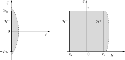
Figure 4: Portion of a black hole space-time in Weyl coordinates (left panel) and Boyer-Lindquist-type coordinates (right panel) (figure taken from [1]).

3.2 The Ernst equation

The complex Ernst potential $f$ combines the metric functions $U$ and $b$,

$$f=\mathrm{e}^{2U}+\mathrm{i}b\,,$$ (24)

where the twist potential $b$ is related to the coefficient $a$ via the relations:

$$a_{,\rho}=\rho\,\mathrm{e}^{-4U}b_{,\zeta},\qquad a_{,\zeta}=-\rho\,\mathrm{e}^{-4U}b_{,\rho}.$$ (25)

In Boyer-Lindquist-type coordinates, this relation reads as:

$$a_{,R}=-2\sin\theta\,\mathrm{e}^{-4U}b_{,\theta},\qquad a_{,\theta}=2(R^{2}-r_{\mathrm{h}}^{2})\sin\theta\,\mathrm{e}^{-4U}b_{,R}.$$ (26)

The vacuum Einstein equations (which are valid in a vicinity of $\mathcal{H}^{+}$) are equivalent to the Ernst equation [5] which reads in Weyl coordinates as

$$(\Re f)\left(f_{,\rho\rho}+f_{,\zeta\zeta}+\frac{1}{\rho}f_{,\rho}\right)=f_{,\rho}^{2}+f_{,\zeta}^{2}$$ (27)

and in Boyer-Lindquist-type coordinates:

$$(\Re f)\left[(R^{2}-r_{\mathrm{h}}^{2})f_{,RR}+2Rf_{,R}+f_{,\theta\theta}+\cot\theta f_{,\theta}\right]=(R^{2}-r_{\mathrm{h}}^{2})f_{,R}^{2}+f_{,\theta}^{2}.$$ (28)

Note that because of the degeneracy of $\mathcal{H}^{+}$ in Weyl coordinates, the potential $f$ is, for $\rho=0$, only a $C^{0}$-function in terms of $\zeta$. In contrast, for a regular black hole, $f$ is analytic with respect to the Boyer-Lindquist-type-coordinates $R$ and $\theta$.

3.3 Bäcklund transformation

The Ernst equation is, when written in Weyl coordinates, the integrability condition of an associated linear matrix problem [6, 7]. This is the great advantage of the Weyl coordinates with respect to the Boyer-Lindquist-type coordinates. The existence of this linear problem enables us to apply methods known from soliton theory. In this contribution, we are particularly interested in the so-called Bäcklund transformations through which new solutions from previously known ones are created [8]–[12]. As an example, the Kerr solution describing a rotating black hole in vacuum can be constructed from the flat Minkowski metric in this manner (see e. g. [10]).

In the following we use the Bäcklund transformation technique in order to write an arbitrary regular axisymmetric, stationary black hole solution $f$ in terms of an auxiliary ‘seed’ potential $f_{0}$. Here, $f_{0}$ describes a space-time without a black hole but with a completely regular central vacuum region. More specifically, $f_{0}$ is characterized by the following properties:

1. $f_{0}$ is defined in a vicinity of the axis section $\rho=0,|\zeta|\leq 2r_{\mathrm{h}}$.

2. In this vicinity, $f_{0}$ is an analytic function of $\rho$ and $\zeta$ and an even function of $\rho$.

3. For $\rho=0$ and $|\zeta|\leq 2r_{\mathrm{h}}$, the values of $f_{0}$ in terms of the event horizon values of $f$ are given by

   $$f_{0}=\frac{\mathrm{i}\left[2r_{\mathrm{h}}(b^{+}_{\mathrm{N}}+b^{+}_{\mathrm{S}})-(b^{+}_{\mathrm{N}}-b^{+}_{\mathrm{S}})\zeta\right]f+4r_{\mathrm{h}}b^{+}_{\mathrm{N}}b^{+}_{\mathrm{S}}}{4r_{\mathrm{h}}f-\mathrm{i}\left[2r_{\mathrm{h}}(b^{+}_{\mathrm{N}}+b^{+}_{\mathrm{S}})+(b^{+}_{\mathrm{N}}-b^{+}_{\mathrm{S}})\zeta\right]},$$ (29)

   where $b^{+}_{\mathrm{N}}=b(\rho=0,\zeta=2r_{\mathrm{h}})$ and $b^{+}_{\mathrm{S}}=b(\rho=0,\zeta=-2r_{\mathrm{h}})$ denote the twist potential values at north and south poles of $\mathcal{H}^{+}$.

Now, from this Ernst potential $f_{0}$ the original potential $f$ can be recovered by means of an appropriate Bäcklund transformation of the following form:

$$f=\frac{\left|\begin{array}[]{ccc}f_{0}&1&1\\ \bar{f}_{0}&\alpha_{1}\lambda_{1}&\alpha_{2}\lambda_{2}\\ f_{0}&\lambda_{1}^{2}&\lambda_{2}^{2}\end{array}\right|}{\left|\begin{array}[]{ccc}1&1&1\\ -1&\alpha_{1}\lambda_{1}&\alpha_{2}\lambda_{2}\\ 1&\lambda_{1}^{2}&\lambda_{2}^{2}\end{array}\right|},$$ (30)

where

$$\lambda_{j}=\sqrt{\frac{K_{j}-\mathrm{i}\bar{z}}{K_{j}+\mathrm{i}z}},\qquad j=1,2,\qquad K_{1}=-2r_{\mathrm{h}},\qquad K_{2}=2r_{\mathrm{h}}$$ (31)

with the complex coordinates $z=\rho+\mathrm{i}\zeta$, $\bar{z}=\rho-\mathrm{i}\zeta$, and $\alpha_{1}$, $\alpha_{2}$ are solutions to the Riccati equations

$$\alpha_{j,z} = -(\lambda_{j}\alpha_{j}^{2}+\alpha_{j})\frac{f_{0,z}}{f_{0}+\bar{f}_{0}}+(\alpha_{j}+\lambda_{j})\frac{\bar{f}_{0,z}}{f_{0}+\bar{f}_{0}},$$ (32)

$$\alpha_{j,\bar{z}} = -\left(\frac{1}{\lambda_{j}}\alpha_{j}^{2}+\alpha_{j}\right)\frac{f_{0,\bar{z}}}{f_{0}+\bar{f}_{0}}+\left(\alpha_{j}+\frac{1}{\lambda_{j}}\right)\frac{\bar{f}_{0,\bar{z}}}{f_{0}+\bar{f}_{0}}$$ (33)

with

$$\alpha_{j}\bar{\alpha}_{j}=1.$$ (34)

For a regular black hole, $f$ is analytic with respect to $R$ and $\cos\theta$ in an exterior vicinity of ${\cal H}^{+}$. Hence, we can expand it analytically into an interior vicinity of $\mathcal{H}^{+}$. A theorem by Chruściel (theorem 6.3 in [13]) assures that the potential $f$ exists as a regular solution of the interior Ernst equation for all values

$$(R,\cos\theta)\in(-r_{\mathrm{h}},r_{\mathrm{h}}]\times[-1,1]\,.$$ (35)

This region only excludes the Cauchy horizon $\mathcal{H}^{-}$ ($R=-r_{\mathrm{h}}$).

In the following derivation of the expression for $f$ at the interior boundary $R=-r_{\mathrm{h}}$, a crucial role is played by the fact that $f_{0}$ is even in $\rho$. In terms of the Boyer-Lindquist-type coordinates, this means that $f_{0}$ is an analytic function of $(R^{2}-r_{\mathrm{h}}^{2})\sin^{2}\!\theta$ and $R\cos\theta$. The analytic expansion of $f_{0}$ into the region $R<r_{\mathrm{h}}$ retains this property. Hence, $f_{0}$ taken at the boundaries of the inner hyperbolic region, can be expressed in terms of $f_{0}$ taken at $R=r_{\mathrm{h}}$. Specifically we obtain

$$f_{0}(R=\,-\,r_{\mathrm{h}}\,,\cos\theta)=f_{0}(R=\,+\,r_{\mathrm{h}}\,,-\cos\theta)=f_{0}(\rho=0,\zeta=-2r_{\mathrm{h}}\cos\theta)\,.\,$$ (36)

Also, it follows that $f_{0}$ is regularly defined in a sufficiently small vicinity of the boundary of the interior region, see figure 5.

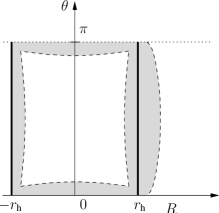
Figure 5: The seed function $f_{0}$ can be regularly defined in at least the grey areas (figure taken from [1]).

From the values of $f_{0}$ at these boundaries we can construct $f$ on $\mathcal{H}^{-}$ via the Bäcklund transformation, which is stated in the following.

Theorem 3.1.

Any Ernst potential $f$ of a regular, axisymmetric, and stationary black hole space-time with angular momentum $J\neq 0$, can be regularly extended into the interior of the black hole up to and including an interior Cauchy horizon, described by $R=-r_{\mathrm{h}}$ in Boyer-Lindquist-type coordinates $(R,\theta)$. The values of $f$ on the Cauchy horizon are given by

$$\fl f(R=-r_{\mathrm{h}},\cos\theta)=\frac{\mathrm{i}\left[\delta_{1}+\delta_{2}-(\delta_{1}-\delta_{2})\cos\theta\right]f_{0}(R=r_{\mathrm{h}},-\cos\theta)+2\delta_{1}\delta_{2}}{2f_{0}(R=r_{\mathrm{h}},-\cos\theta)-\mathrm{i}\left[\delta_{1}+\delta_{2}+(\delta_{1}-\delta_{2})\cos\theta\right]}$$ (37)

with

$$\delta_{1}=\frac{b^{+}_{\mathrm{S}}(b^{+}_{\mathrm{N}}-b^{+}_{\mathrm{S}})+2b^{+}_{\mathrm{N}}(b_{,\theta\theta})^{+}_{\mathrm{N}}}{b^{+}_{\mathrm{N}}-b^{+}_{\mathrm{S}}+2(b_{,\theta\theta})^{+}_{\mathrm{N}}},\qquad\delta_{2}=\frac{b^{+}_{\mathrm{N}}(b^{+}_{\mathrm{N}}-b^{+}_{\mathrm{S}})+2b^{+}_{\mathrm{S}}(b_{,\theta\theta})^{+}_{\mathrm{N}}}{b^{+}_{\mathrm{N}}-b^{+}_{\mathrm{S}}+2(b_{,\theta\theta})^{+}_{\mathrm{N}}}$$ (38)

where the scripts ‘+’ and ‘N/S’ indicate that the corresponding value of $b$ or its second $\theta$-derivative has to be taken at the event horizon’s north or south pole respectively. The values of the seed solution $f_{0}$ for $R=r_{\mathrm{h}}$ follow via f0 from $f$ on the event horizon.

Note that, for $J\to 0$, the Cauchy horizon becomes singular. In this case we have $|\delta_{1/2}|\to\infty$ and consequently $f|_{\mathcal{H}^{-}}$ diverges.

By virtue of the above theorem we are able to write the inner Cauchy horizon area $A^{-}$ completely in terms of Ernst expressions taken at the event horizon $\mathcal{H}^{+}$. As discussed in [1], the universal equality (1) arises in this manner. Moreover, the vanishing of $A^{-}$ is obtained in the limit $J\to 0$, i. e. when the Cauchy horizon becomes singular.

4 Discussion

In this contribution we discussed the interior hyperbolic region of axisymmetric and stationary black holes which are surrounded by a matter distribution. We first looked at the corresponding degenerate hyperbolic Einstein equations in terms of fully pseudo-spectral methods, and confirmed the validity of relation (1) to high precision.

In the second part of the article, we used the Bäcklund technique in order to write the black hole metric in terms of an auxiliary seed potential $f_{0}$ that does not describe a black hole but a completely regular central region. We first derived simple relations between the values of $f_{0}$ at the boundaries of the interior region, and then carried these relations over to the original black hole metric by virtue of an appropriate Bäcklund transformation. A particular consequence of this relation is the universal equality (1).

Note that the key point for this method to work is the fact that the two horizons $\mathcal{H}^{\pm}$ are connected by specific axis sections. Indeed, the linear matrix problem associated to the Ernst equation (see discussion at the beginning of section 3.3) simplifies considerably for $\rho=0$, that is, on the two horizons $\mathcal{H}^{\pm}$, and on the rotation axis ($\sin\theta=0$). An alternative derivation, analyzing the linear matrix problem directly at the several sections where $\rho=0$, was carried out in [14, 15] for the Einstein-Maxwell field. In that work, the corresponding steps yield the more general formula

$$(8\pi J)^{2}+(4\pi Q^{\,2})^{2}=A^{+}A^{-}$$

where $Q$ is the electric charge of the black hole.

It is interesting to remark that there are associated inequalities relating angular momentum and area of the black hole. In [16] (see also [17]) it was shown that for subextremal black holes (which possess trapped surfaces in every sufficiently small interior vicinity of the event horizon), the following inequalities hold:

$$A^{-}<\sqrt{(8\pi J)^{2}+(4\pi Q^{\,2})^{2}}<A^{+}.$$

In the case of pure Einsteinian gravity, this relation was proved in a different context, namely for non-stationary, axisymmetric, vacuum space-times [18]. In particular, the local inequality $A\geq 8\pi|J|$ was shown, where $A$ and $J$ are the area and angular momentum of any axially symmetric closed stable minimal surface in an axially symmetric maximal initial data.

We would like to thank S. Dain and P. T. Chruściel for illuminating discussions and Robert Thompson for commenting on the manuscript.

References

References

• [1] Ansorg M and Hennig J 2008 The inner Cauchy horizon of axisymmetric and stationary black holes with surrounding matter Class. Quant. Grav. 25 222001
• [2] Carter B 1973 Black hole equilibrium states, in Black Holes (Les Houches) ed C deWitt and B deWitt (London: Gordon and Breach) pp 57-214
• [3] Bardeen J M 1973 Rapidly rotating stars, disks, and black holes, in Black holes (Les Houches) ed C deWitt and B deWitt (London: Gordon and Breach) pp 241-289
• [4] Hennig J and Ansorg M 2009 A Fully Pseudospectral Scheme for Solving Singular Hyperbolic Equations Journal of Hyperbolic Differential Equations 6 161
• [5] Ernst F J 1968 New Formulation of the Axially Symmetric Gravitational Field Problem Phys. Rev. 167 1175
• [6] Neugebauer G 1979 Bäcklund transformations of axially symmetric stationary gravitational fields Journal of Physics A 12 L67
• [7] Neugebauer G 1980 A general integral of the axially symmetric stationary Einstein equations Journal of Physics A 13 L19
• [8] Harrison B K 1978 Bäcklund Transformation for the Ernst Equation of General Relativity Phys. Rev. Lett. 41 1197
• [9] Kramer D and Neugebauer G 1983 Bäcklund transformations in General Relativity in Proc. of the Int. Seminar on Solutions of Einstein’s Equations (Retzbach) ed Hoenselaers C and Dietz W (Berlin: Springer-Verlag) pp 1-25
• [10] Neugebauer G 1996 Gravitostatics and Rotating Bodies in Proc. of the 46th Scottish Universities Summer School in Physics (Aberdeen) ed Hall G S and Pulham J R (London: IOP) pp 61-81
• [11] Ansorg M. 2001 Differentially Rotating Disks of Dust: Arbitrary Rotation Law Gen. Rel. Grav. 33 309
• [12] Ansorg M., Kleinwächter A., Meinel R. and Neugebauer G. 2002 Dirichlet Boundary Value Problems of the Ernst Equation Phys. Rev. D 65 044006
• [13] Chruściel P T 1990 On space-times with $U(1)\times U(1)$ symmetric compact Cauchy surfaces Ann. Physics 202 100
• [14] Ansorg M and Hennig J 2009 Inner Cauchy horizon of axisymmetric and stationary black holes with surrounding matter in Einstein-Maxwell theory Phys. Rev. Lett. 102 221102
• [15] Hennig J and Ansorg M 2009 The inner Cauchy horizon of axisymmetric and stationary black holes with surrounding matter in Einstein-Maxwell theory: study in terms of soliton methods Annales Henri Poincare 10 1075
• [16] Hennig J, Cederbaum C and Ansorg M 2010 A universal inequality for axisymmetric and stationary black holes with surrounding matter in the Einstein-Maxwell theory Comm. Math. Phys. 293 449
• [17] Hennig J, Ansorg M. and Cederbaum C 2008 A universal inequality between angular momentum and horizon area for axisymmetric and stationary black holes with surrounding matter Class. Quant. Grav. 25 162002
• [18] Dain S and Reiris M Area - Angular momentum inequality for axisymmetric black holes arXiv:1102.5215