Hubble expansion and structure formation in the “running FLRW model” of the cosmic evolution

Abstract:

A new class of Friedmann-Lemaître-Robertson-Walker (FLRW) cosmological models with time-evolving fundamental parameters should emerge naturally from a description of the expansion of the universe based on the first principles of quantum field theory and string theory. Within this general paradigm, one expects that both the gravitational Newton’s coupling $G$ and the cosmological term $\Lambda$ should not be strictly constant but appear rather as smooth functions of the Hubble rate $H(t)$. This scenario (“running FLRW model”) predicts, in a natural way, the existence of dynamical dark energy without invoking the participation of extraneous scalar fields. In this paper, we perform a detailed study of some of these models in the light of the latest cosmological data, which serves to illustrate the phenomenological viability of the new dark energy paradigm as a serious alternative to the traditional scalar field approaches. By performing a joint likelihood analysis of the recent supernovae type Ia data (SNIa), the Cosmic Microwave Background (CMB) shift parameter, and the Baryonic Acoustic Oscillations (BAOs) traced by the Sloan Digital Sky Survey (SDSS), we put tight constraints on the main cosmological parameters. Furthermore, we derive the theoretically predicted dark-matter halo mass function and the corresponding redshift distribution of cluster-size halos for the “running” models studied. Despite the fact that these models closely reproduce the standard $\Lambda$CDM Hubble expansion, their normalization of the perturbation’s power-spectrum varies, imposing, in many cases, a significantly different cluster-size halo redshift distribution. This fact indicates that it should be relatively easy to distinguish between the “running” models and the $\Lambda$CDM using realistic future X-ray and Sunyaev-Zeldovich cluster surveys.

1 Introduction

The high-quality observations performed during the last two decades have enabled cosmologists to gain substantial confidence that modern cosmology is capable of quantitatively reproducing the details of the many observed cosmic phenomena [1, 2, 3], including the accelerated expansion of the universe at the present epoch [4]. The field of cosmology, therefore, is no longer a pure realm of philosophical speculation, but a rigorous branch of experimental physics. In view of this fact, the status of modern cosmology can be declared as very healthy and highly satisfactory from the point of view of the empirical sciences. Nevertheless, if we pause for a moment and make a deeper reflection, we soon come to realize that the ultimate understanding of these magnificent observations is still highly blurred, if not completely opaque, to the light of the first principles of fundamental theoretical physics, e.g. from the viewpoint of Quantum Field Theory (QFT) and string theory.

Indeed, we realize that what we have been able to do throughout the last decade is to furnish a rather precise numerical fit to the parameters of the Friedmann-Lemaître-Robertson-Walker (FLRW) model in the light of the most accurate observations, but at the moment these observational successes are not accompanied by a deeper theoretical insight into the meaning of the preciously collected data on dark matter (DM) and dark energy (DE). Needless to say, the resulting high quality of this combined fit (from independent data sources) speaks very well for the FLRW model as a likely correct starting point to understand the structure of our cosmos. However, it does not provide a single clue to the meaning of – or on the physical substratum lying underneath – the fitted energy density parameters at the present time $\Omega_{m}^{0}$ and $\Omega_{\Lambda}^{0}$ (except for the baryonic part $\Omega_{b}^{0}\simeq 0.04$, of course, which we know from primordial nucleosynthesis), nor does it explain why the geometric parameter $\Omega_{K}^{0}$ is comparatively much smaller. In practice, observations tell us that $\Omega_{m}^{0}\simeq 0.28$ and $\Omega_{\Lambda}^{0}\simeq 0.72$ (with $\Omega_{K}^{0}\lesssim 0.01$. It follows that most of the matter content of the universe is non-baryonic DM, and that the value of the cosmological constant density $\rho_{\Lambda}^{0}=\Lambda/(8\pi G)$, or, in general, the current dark energy (DE) density, is

$$\rho_{\Lambda}^{0}=\Omega_{\Lambda}^{0}\,\rho_{c}^{0}\simeq 6\,h^{2}\times 10^{-47}\,\rm{GeV}^{4}\simeq 3\times 10^{-47}\,\rm{GeV}^{4}\,,$$ (1)

where $\rho_{c}^{0}\simeq\left(3.0\,\sqrt{h}\times 10^{-12}\,\rm{GeV}\right)^{4}\sim 4\times 10^{-47}$ GeV⁴ is the present value of the critical density and $H_{0}=100\,h$ km/s/Mpc, with $h\simeq 0.704$, the current Hubble’s rate.

Despite the “scandal” of our having to admit full ignorance about the identity of most ($\sim 90\%$) of the matter budget of the universe, this trouble pales in comparison to the colossal enigma hidden behind the value (1). Understanding this value is perhaps the biggest scientific mystery of all times: “the cosmological constant problem” [5, 6], which manifests itself as the double conundrum of the tiny observed value of the cosmological constant (CC) in Einstein’s equations – the “old CC problem” [7] –, and also the puzzling fact that this value is so close to the current matter density (the “cosmic coincidence problem” [8]), including the mystery of a possible phantom behavior near our time. Solving these problems surely requires introducing new fundamental ideas of profound theoretical meaning and scope. Some promising new avenues have recently been proposed [9, 10, 11, 12, 13] – see also the recent alternative attempts [15, 16, 17, 18].

For a long time model builders have pursued an explanation of these cosmological puzzles in terms of dynamical scalar fields [19], later adapted into the idea of quintessence [20]. Quintessence was proposed without attempting to explain the smallness of the CC, but only to cope with some aspects of the cosmic coincidence problem [6]. These scalar field models ignore ab initio the huge vacuum energy from the Standard Model (SM) of strong and electroweak interactions, which is $55$ orders of magnitude larger than the measured value (1) — see [9] (section 2 and Appendix B) for a very detailed discussion. Moreover, quintessence models usually postulate a preposterously tiny mass for these scalar fields of the order of $10^{-33}$ eV, i.e. comparable to the current Hubble rate $H_{0}$. This is a great disadvantage, not to mention the fact that they are plagued with the same fine tuning problems as the original CC approach itself, as emphasized in [9].

From our point of view, a sensible possibility that should not be neglected is to think of a “dynamical $\Lambda$” or “effective vacuum energy” $\rho_{\Lambda{\rm eff}}$, where, rather than replacing $\Lambda$ by a collection of ad hoc ersatz fields, we stick to the idea that the CC term in Einstein’s equations is still a “true cosmological term”, although we permit that “the observable CC at each epoch” can be an effective quantity evolving with the expansion of the universe: $\rho_{\Lambda{\rm eff}}=\rho_{\Lambda{\rm eff}}(H)$, where $H$ is the Hubble rate. While the old phenomenological models for time-evolving CC  [21, 22] lacked of a fundamental motivation, a general dynamical $\Lambda$ approach within QFT has more recently been emphasized in [23, 24, 25, 26] and also in the past from the point of view of QFT in curved space-time – see   [12] and [27, 28, 29].

The more modern idea of a slowly running CC is based on the possibility that quantum effects in curved space-time [30] can be responsible for the renormalization group (RG) running of the vacuum energy. One can show that these models [14] are nicely compatible with the most recent experimental data [31], and this fact spurs us to further explore their impact both in the cosmological and astrophysical domain. We shall concentrate here on a class of RG models in which the vacuum energy is a function of cosmic time $t$ though the Hubble rate $H=H(t)$. An archetype example is the quantum field vacuum model based on the evolution law $\Lambda(H)=n_{0}+n_{2}\,H^{2}$. In Ref. [31] some of us have investigated the global dynamics of this cosmological model (together with various alternative $\Lambda(t)$ models), in the light of the most recent cosmological data. However, in that paper we assumed that the vacuum decayed into matter, whereas here we wish to explore the complementary possibility that matter is conserved thanks to a logarithmically variable gravitational coupling $G=G(H)$. This is very appealing because, if matter is conserved, then one cannot run into potential problems related with the fact that the vacuum energy could decay in part into baryons and photons, which would be of course undesirable. We shall call such FLRW-like model, with $G=G(H)$ and $\Lambda=\Lambda(H)$, the “running FLRW model” (hereafter $\Lambda_{t}G_{t}$CDM), in contrast to the “running $\Lambda$CDM model” (denoted $\Lambda_{t}$CDM) in which only $\Lambda$ evolves with time at the expense of maintaining an interaction with matter [28].

In this paper, we wish to test the two basic types of running models in the light of the most recent cosmological data on SNIa+BAO+CMB (i.e., distant type Ia supernovae, baryonic acoustic oscillations and cosmic microwave background anisotropies). The clustering properties of the vacuum energy can also be of high interest as they may help to shed some light on the fundamental issue of non-linear structure formation. The subject has been discussed for different DE models, although mainly based on scalar fields [32]-[33] (and references therein). A first study in this direction for running vacuum models was recently presented by some of us in [41]. In the current work, however, we emphasize on the implications for the formation and distribution of the collapsed cosmic structures (i.e. galaxy clusters) along the lines of the methods utilized in [31], which we apply here to the $\Lambda_{t}G_{t}$CDM model, and leave the presentation of the clustering effects in this model for a separate work. Therefore, we focus here on the study of the dark-matter halo mass function and the redshift distribution of cluster-size halos, and compare with the corresponding results for the $\Lambda_{t}G_{t}$CDM and the concordance $\Lambda$CDM model.

The paper is organized as follows. In the next section, we discuss some scenarios with variable $\Lambda$ and $G$. In Sect. 3, the FLRW model with running $G$ and $\Lambda$ (i.e. the $\Lambda_{t}G_{t}$CDM model) is introduced, while in Sect. 4 we review the $\Lambda_{t}$CDM model. The confrontation of these models with the latest cosmological data is made in Sect. 6, and their predictions concerning the formation of the galaxy cluster-size halos and the evolution of their abundance is presented in Sect. 7. In the last section, we deliver our conclusions. Finally, in an appendix we provide details of the calculation of the linearly extrapolated critical density for the RG models under consideration.

2 Models with time-evolving cosmological parameters

The idea that the vacuum energy should not be a ‘rigid’ quantity in cosmology is a most natural one [14]. It is difficult to conceive an expanding universe with a strictly constant CC energy density, $\rho_{\Lambda}=\Lambda/(8\pi\,G)$, namely one that has remained immutable since the origin of time. A smoothly-evolving vacuum energy $\rho_{\Lambda}=\rho_{\Lambda}(t)$ that inherits its time-dependence from cosmological functions such as the scale factor $a(t)$ or the Hubble rate $H(t)$, is not only a qualitatively more plausible and intuitive idea, but is also suggested by fundamental physics, in particular by quantum field theory (QFT) in curved space-time [30]. To implement this notion, it is not strictly necessary to resort to ad hoc scalar fields, as usually done in the literature (e.g. in quintessence formulations and the like [20]). A “running” $\Lambda$ term can be expected on very similar grounds as one expects (and observes) the running of couplings and masses with a physical energy scale in QFT.

Therefore, the guiding paradigm that we adopt in this paper is that the CC density should naturally be a function of the cosmic time $t$, or equivalently of the cosmological redshift $z$. The generalization of this possibility to all the cosmological parameters, with an eye on trying to explain many surprising features of the dark energy (DE) – such as the apparent phantom-like behavior near our time – has been put forward in [12]. Within this context, all the cosmological parameters are viewed as effective couplings whose running can be studied from the semi-classical formulation of QFT in curved space-time [30]. Interestingly enough, the possibility to derive this evolution from an effective action has also been addressed in some particular cases [23, 42]. Let us also remark that these ideas have been pursued in the literature from different points of view since long ago [43, 27, 28, 29, 44], and they have been recently re-examined both from the theoretical point of view [24] and also from the viewpoint of various kinds of possible phenomenological implications [31, 45, 41, 46, 47].

In this framework, the variation of “fundamental constants” such as $\Lambda$ and $G$ could emerge as an effective description of some deeper dynamics associated to QFT in curved space-time, or quantum gravity or even string theory, all of which share the powerful renormalization group (RG) approach. The latter entails the possibility to analyze the potential impact of the leading quantum effects from matter particles on the cosmological observables such as vacuum energy and gravitational coupling. These effects should eventually lead to definite time-evolution laws $\rho_{\Lambda}=\rho_{\Lambda}(t)\,,G=G(t)$. However, given a fundamental model based on QFT, the parameter $\rho_{\Lambda}$ will primarily depend on some cosmological functions (matter density $\rho_{m}$, Hubble expansion rate $H$, etc) which evolve with time or redshift. Similarly for the Newton coupling $G$. Therefore, in general we will have the two following functions of the cosmic time or the cosmological redshift [12]:

$$\rho_{\Lambda}(z)=\rho_{\Lambda}(\rho_{m}(z),H(z),...)\,,\ \ \ \ \ G(z)=G(\rho_{m}(z),H(z),...)\,.$$ (2)

Of course, other fundamental parameters could also be variable. For example, the fine structure constant has long been speculated as being potentially variable with the cosmic time (and therefore with the redshift) including some experimental evidences – see e.g.  [48]. This might also have an interpretation in terms of the RG at the level of the cosmological evolution. However, in this paper we concentrate purely on the potential variability of the most genuinely fundamental gravitational parameters of Einstein’s equations such as $\Lambda$ and $G$. The possibility that $G$ could be variable has been previously entertained in the literature, although most of these formulations are usually framed within the original Jordan and Brans-Dicke proposals [49] linked to the existence of a dynamical scalar field coupled to curvature.

The cosmological constant contribution to the curvature of space-time is represented by the $\Lambda\,g_{\mu\nu}$ term on the l.h.s. of Einstein’s equations, which can be absorbed on the r.h.s. of these equations:

$$R_{\mu\nu}-\frac{1}{2}g_{\mu\nu}R=8\pi G\ \tilde{T}_{\mu\nu}\,,$$ (3)

where the modified energy-momentum tensor is given by $\tilde{T}_{\mu\nu}\equiv T_{\mu\nu}+g_{\mu\nu}\,\rho_{\Lambda}$. Here $\rho_{\Lambda}=\Lambda/(8\pi G)$ is the vacuum energy density associated to the presence of $\Lambda$, and $T_{\mu\nu}$ is the ordinary energy-momentum tensor of isotropic matter and radiation. Modeling the expanding universe as a perfect fluid with velocity $4$-vector field $U^{\mu}$, we have $T_{\mu\nu}=-p_{m}\,g_{\mu\nu}+(\rho_{m}+p_{m})U_{\mu}U_{\nu}$, where $\rho_{m}$ is the proper isotropic density of matter-radiation and $p_{m}$ is the corresponding pressure. Clearly the modified $\tilde{T}_{\mu\nu}$ defined above takes the same form as ${T}_{\mu\nu}$ with $\tilde{\rho}=\rho_{m}+\rho_{\Lambda}$ and $\tilde{p}=p_{m}-\rho_{\Lambda}$. Therefore:

$$\tilde{T}_{\mu\nu}=-\tilde{p}\,g_{\mu\nu}+(\tilde{\rho}+\tilde{p})U_{\mu}U_{\nu}=(\rho_{\Lambda}-p_{m})\,g_{\mu\nu}+(\rho_{m}+p_{m})U_{\mu}U_{\nu}\,.$$ (4)

With this generalized energy-momentum tensor, and in the spatially flat FLRW metric $ds^{2}=dt^{2}-a^{2}(t)d\vec{x}^{2}$, the gravitational field equations boil down to Friedmann’s equation

$$H^{2}\equiv\left(\frac{\dot{a}}{a}\right)^{2}=\frac{8\pi\,G}{3}\tilde{\rho}=\frac{8\pi\,G}{3}\left(\rho_{m}+\rho_{\Lambda}\right)\,,$$ (5)

and the dynamical field equation for the scale factor:

$$\ddot{a}=-\frac{4\pi}{3}G\,(\tilde{\rho}+3\,\tilde{p})\,a=-\frac{4\pi}{3}G\,(\rho_{m}+3\,p_{m}-2\,\rho_{\Lambda})\,a\,.$$ (6)

Let us next contemplate the possibility that $G=G(t)$ and $\rho_{\Lambda}=\rho_{\Lambda}(t)$ can be both functions of the cosmic time. This is allowed by the Cosmological Principle embodied in the FLRW metric. The Bianchi identities (which insure the covariance of the theory) then imply $\bigtriangledown^{\mu}\,\left({G\,\tilde{T}}_{\mu\nu}\right)=0$. In the case of the FLRW metric, the previous identity amounts to the following generalized local conservation law:

$$\frac{d}{dt}\,\left[G(\rho_{\Lambda}+\rho_{m})\right]+3\,G\,H\,(\rho_{m}+p_{m})=0\,.$$ (7)

This equation is actually a first integral of the dynamical system (5) and (6), as can be easily checked. When $G$ is constant, the identity above implies that $\rho_{\Lambda}$ is also a constant, if and only if the ordinary energy-momentum tensor is individually conserved ($\bigtriangledown^{\mu}\,{T}_{\mu\nu}=0$), i.e. $\dot{\rho}_{m}+3\,H\,(\rho_{m}+p_{m})=0$. This equation can be rewritten

$${\rho}_{m}^{\prime}(a)+\frac{3}{a}\,(\rho_{m}(a)+p_{m}(a))=0\,,$$ (8)

where the prime indicates differentiation with respect to the scale factor: $f^{\prime}=df/da$ for any function $f(a)$. The solution of (8) is

$$\rho_{m}(a)=\rho_{m}^{0}\,a^{-3(1+\omega_{m})}=\rho_{m}^{0}\,(1+z)^{3(1+\omega_{m})}$$ (9)

where $\rho_{m}^{0}$ is the current matter density and $\omega_{m}=p_{m}/\rho_{m}$ is the equation of state (EoS) parameter for cold ($\omega_{m}=0$) and relativistic ($\omega_{m}=1/3$) matter, respectively. We have expressed the result (9) in terms of the scale factor $a=a(t)$ and the cosmological redshift $z=(1-a)/a$.

A first non-trivial situation appears when $\rho_{\Lambda}=\rho_{\Lambda}(t)$ but $G$ remains still constant. Then equation (7) boils down to

$$\dot{\rho}_{\Lambda}+\dot{\rho}_{m}+3\,H\,(\rho_{m}+p_{m})=0\,,$$ (10)

This scenario shows that a time-variable $\rho_{\Lambda}$ cosmology may exist such that transfer of energy occurs from matter-radiation into vacuum energy, and vice versa (see section 4). However, let us remark that the time evolution of $\rho_{\Lambda}$ is still possible in a framework where matter is strictly conserved, i.e. such that equation (8) is maintained. Such scenario is highly desirable and is perfectly consistent with the Bianchi identity at the expense of a time-varying gravitational coupling: $G=G(t)$. Indeed, it is easy to see that equation (8) is compatible with (7) provided that the following differential constraint between the variable $G$ and the variable $\rho_{\Lambda}$ is satisfied:

$$(\rho_{m}+\rho_{\Lambda})\,d{G}+G\,d{\rho}_{\Lambda}=0\,,$$ (11)

where $\rho_{m}$ in this equation is given by (9). To solve the model in the basic set of variables $(H(z),\rho_{m}(z),p(z),G(z),\rho_{\Lambda}(z))$, still another equation is needed. In the next section we discuss the possibility that the fifth missing equation is a QFT-inspired relation of the form $\rho_{\Lambda}=\rho_{\Lambda}(H(z))$.

3 A FLRW-like model with running $G$ and $\Lambda$: the $\Lambda_{t}G_{t}$CDM model

Consider the class of models in which the vacuum energy and the gravitational coupling evolve as power series of some energy scale $\mu$, such that the rates of change are given respectively by

$$\frac{d\rho_{\Lambda}(\mu)}{d\ln\mu}=\sum_{k=0,1,2,...}\,A_{2k}\,\mu^{2k}\,,\ \ \ \ \ \ \frac{d}{d\ln\mu}\left(\frac{1}{G(\mu)}\right)=\sum_{k=0,1,2,...}\,B_{2k}\,\mu^{2k}\,.$$ (12)

These expansions can be considered as purely phenomenological ansatzs or, if we aim at a more fundamental description, as emerging from the quantum field RG running of the cosmological parameters [27, 28, 46]. Such running should ultimately reflect the dependence of the leading quantum effects on some physical cosmological quantity $\xi$ associated with $\mu$, hence $\rho_{\Lambda}=\rho_{\Lambda}(\xi)$. The physical scale $\xi$ could typically be the Hubble rate $H$, or even the scale factor $a$, which in most of the cosmological past also maps out the evolution of the energy densities with $H$ [23]. Since in both cases $\xi=\xi(t)$ evolves with the cosmic time, the cosmological term inherits a time-dependence through its primary scale evolution with $H(t)$ or $a(t)$. In this context, the r.h.s. of the above equations defines the $\beta$-functions for the running of $\rho_{\Lambda}$ and $G^{-1}$ in QFT in curved space-time. The setting $\mu\to H$ naturally points to the typical energy scale of the classical gravitational external field associated to the FLRW metric, i.e. the characteristic energy of the FLRW “gravitons” attached to the quantum matter loops contributing to the running of $\rho_{\Lambda}$ and $G^{-1}$ in a semi-classical description of gravity. Coefficients $A_{2k},B_{2k}$ in these formulas receive contributions from boson and fermion matter fields of different masses $M_{i}$, and the series (12) become expansions in powers of the small quantities $H/M_{i}$ [28, 29]. The fact that only even powers of $H$ are involved is dictated by the general covariance of the effective action [24, 23] . After integrating the formulas (12), the result may be looked upon as a specific implementation of the general equations (2), where the expansion rate $H$ is singled out as the main cosmological variable on which the functions $\rho_{\Lambda}$ and $G^{-1}$ depend and in terms of which are expanded.

It is important to note that the expansions (12) are correlated by the Bianchi identity (11) and therefore they must be consistent with it, order by order. Let us consider them more closely. We start by first rewriting the expression for the RG of the CC term in a more explicit manner, as follows:

$$\frac{d\rho_{\Lambda}(\mu)}{d\ln\mu}=\frac{1}{(4\pi)^{2}}\left[\sum_{i}\,B_{i}M_{i}^{2}\,\mu^{2}+\sum_{i}\,C_{i}\,\mu^{4}+\sum_{i}\frac{\,D_{i}}{M_{i}^{2}}\,\mu^{6}\,\,+...\right]\equiv 2\,n_{2}\,\mu^{2}+{\cal O}(\mu^{4})\,,$$ (13)

where $M_{i}$ are the masses of the particles contributing in the loops, and $B_{i},C_{i},..$ are dimensionless parameters. We have omitted the $M_{i}^{4}$ terms in the expansion since, as explained in [28, 29], such terms would trigger a too fast running of the CC. It follows that only the “soft-decoupling” terms of the form $\sim M_{i}^{2}\,\mu^{2}$ remain in practice. The integrated form of (13) reads

$$\rho_{\Lambda}(H)=n_{0}+n_{2}H^{2}\,,$$ (14)

where we have set $\mu=H$ and neglected the smaller higher order terms, which are of ${\cal O}(H^{4})$. The additive constant $n_{0}$ in (14) must be essentially given by the current value of the vacuum energy, $\rho_{\Lambda}^{0}$, but not quite. Notice that if $n_{2}=0$, the CC is strictly constant and then $n_{0}$ just coincides with $\rho_{\Lambda}^{0}$. However, if the $H^{2}$ term is to play a significant role while preserving the approximate $\Lambda$CDM behavior, it should neither be negligible nor dominant as compared to $n_{0}$. Being the latter the leading term in the series expansion, it must still be of order $n_{0}\sim\rho_{\Lambda}^{0}$; thus the largest masses $M_{i}$ associated to $n_{2}\sim\sum_{i}B_{i}\,M^{2}_{i}$ should be in the ballpark of the mass $M_{X}$ associated to a typical Grand Unified Theory (GUT) near the Planck scale $M_{P}$ (see below). From the structure of the expansion (13), with $\mu=H$ and $M_{i}\sim M_{X}$, we reconfirm that no other even power $H^{2n}$ (not even $H^{4}$) can contribute significantly on the r.h.s. of equation (14) at any stage of the cosmological history below $M_{X}\lesssim M_{P}$. It is particularly convenient to rewrite the coefficients of (14) as follows:

$$n_{0}=\rho_{\Lambda}^{0}-\frac{3\nu}{8\pi}\,M_{P}^{2}\,H_{0}^{2}\,,\ \ \ \ \ n_{2}=\frac{3\nu}{8\pi}\,M_{P}^{2}\,,$$ (15)

with

$$\nu=\frac{1}{6\pi}\,\sum_{i}B_{i}\frac{M_{i}^{2}}{M_{P}^{2}}\,.$$ (16)

Here, $H_{0}$ is the value of the Hubble rate at present. A most important (dimensionless) parameter of the present framework is $\nu$, given in equation (16). It defines the main coefficient of the $\beta$-function for the running of the vacuum energy [28]. For $\nu=0$, the vacuum energy remains strictly constant, $\rho_{\Lambda}=\rho_{\Lambda}^{0}$, whereas for non-vanishing $\nu$ the evolution law (14) can now be written as 

$$\rho_{\Lambda}(H)=\rho_{\Lambda}^{0}+\frac{3\nu}{8\pi}\,M_{P}^{2}\,(H^{2}-H_{0}^{2})\,.$$ (17)

Let us stress that, in the QFT framework, $\nu$ is naturally expected to be non-vanishing owing to the quantum effects of matter particles. The coefficients $B_{i}$ in (16) can be computed from the quantum loop contributions of fields with masses $M_{i}$, see e.g. [23] for a specific framework. It is customary to write $\nu$ in the compact form

$$\nu=\frac{\sigma}{12\pi}\,\frac{M^{2}}{M_{P}^{2}}\,,$$ (18)

with $M$ an effective mass parameter of order of the average mass of the heavy particles of the underlying GUT, including their multiplicities  [28]. From the expression (16), it is clear that the natural range of that parameter is $|\nu|\ll 1$; and it can be both positive or negative, since $\sigma=\pm 1$ depending on whether bosons or fermions dominate in the sum of loop contributions (16). For instance, if GUT fields with masses $M_{i}$ near $M_{P}$ do contribute, then $|\nu|\lesssim 1/(12\pi)\simeq 2.6\times 10^{-2}$, but in general we expect it to be smaller because the usual GUT scales, say $M_{X}\sim 10^{16}$ GeV, are not that close to $M_{P}\sim 10^{19}$ GeV. By counting heavy particle multiplicities in a typical GUT (i.e. the total number of particles with masses $M_{i}\sim M_{X}$), a natural estimate lies in the range $\nu=10^{-5}-10^{-3}$  [23].

Clearly, the vacuum energy density (17) is normalized to the present value, i.e.

$$\rho_{\Lambda}(H_{0})=\rho_{\Lambda}^{0}\equiv\frac{3}{8\pi}\,\Omega_{\Lambda}^{0}\,H^{2}_{0}\,M_{P}^{2}\,.$$ (19)

Recall that the observed numerical value of this expression is given by equation (1), corresponding to $\Omega_{\Lambda}^{0}\simeq 0.7$. We remark that the parametrization (17) satisfies the aforementioned condition that $n_{0}$ is the leading term and is of order $\rho_{\Lambda}^{0}$, and at the same time the correction term is of order $M^{2}\,H^{2}$, with $M\sim\sqrt{\nu}\,M_{P}$ a large mass, even if $\nu$ is as small as, say, $|\nu|\sim 10^{-3}$ or less.

What about the running equation for $G^{-1}$ in equation (12)? A more detailed form for it reads:

$$\frac{d}{d\ln\mu}\left(\frac{1}{G}\right)=\sum_{i}\,a_{i}\,M_{i}^{2}+\sum_{i}\,b_{i}\mu^{2}+\sum_{i}\,c_{i}\,\frac{\mu^{4}}{M_{i}^{2}}+...$$ (20)

If we take again $\mu=H$, then, since we have $H\ll M_{i}$ for all the relevant epochs of the universe – at and below the GUT scale –, this series should converge extremely fast, the first term being the dominant one and the remaining terms are inessential. The first term is of course a contribution to the running of $G^{-1}$ which is directly driven by the heavy particle masses $M_{i}$ of the GUT, and therefore can be parametrized as a coefficient times the Planck mass. Thus, we are essentially led to a RGE of the type

$$\frac{d}{d\ln\mu}\left(\frac{1}{G}\right)=2\,\nu\,M_{P}^{2}+...\,,$$ (21)

where the coefficient in front of $M_{P}$ has been fixed by the condition that this solution is compatible with the Bianchi identity (11) after we adopt the solution (17) for the evolution of the vacuum energy and set $\mu=H$, too, for the running $G$ (see below). We shall show below explicitly this consistency, but let us first notice that the solution of (21) satisfying the boundary condition $G(\mu=H_{0})=G_{0}\equiv 1/M_{P}^{2}$ is

$$g(H)\equiv\frac{G(H)}{G_{0}}=\frac{1}{1+\nu\,\ln\left(H^{2}/H_{0}^{2}\right)}\,.$$ (22)

We see that $g(H)$ depends on the parameter $\nu$ and that, to first order, we have $g(H)=1+{\cal O}(\nu)$, i.e. $G(H)=G_{0}(1+{\cal O}(\nu))$. Thus, $\nu$ plays also (in a very evident manner here) the role of the $\beta$-function for the RG running of $G$. For example, for $\nu>0$ the gravitational coupling decreases with the characteristic cosmological energy $H$ (hence $G$ increases with the expansion); it follows that for $\nu>0$ the coupling $G$ is asymptotically free (as the QCD coupling at high energies), whereas for $\nu<0$ the gravitational coupling behaves as the electromagnetic one, i.e. increases with the energy (equivalently, $G$ decreases in this case with the expansion). In both cases the running of $G$ is extremely slow, since it is logarithmic and with a very small coefficient $|\nu|\ll 1$. Let us note that if we would have omitted the leading $\sim M_{i}^{2}$ term on the r.h.s. of equation (20) – as we have done with the $M_{i}^{4}$ term on the r.h.s. of equation (13) – we would have obtained a still slower running of the gravitational coupling:

$$g(H)=\frac{1}{1+\xi\,\,(H^{2}-H_{0}^{2})/M_{P}^{2}}\,,$$ (23)

where $\xi$ is a dimensionless coefficient. In deriving equation (23) we have assumed that the r.h.s. of (20) is dominated by the next-to-leading term $\sim H^{2}$ (for $\mu=H$) under the assumption that the $\sim M_{i}^{2}$ terms cancel. Since $H^{2}/M_{P}^{2}$ is utterly negligible, this new running law for $G$ is even less sensitive to time evolution for the present universe. In this case, the corresponding evolution of the CC following from the Bianchi identity (11) would also be very mild:

$$\rho_{\Lambda}(H)=\rho_{\Lambda}^{0}+\frac{3\xi}{16\,\pi}\,\left(H^{4}-H_{0}^{4}\right)\,.$$ (24)

However, since there is no a priori theoretical reason nor a phenomenological constraint to assume that the leading term $\sim M_{i}^{2}$ terms cancel, we shall concentrate here only on the form (22) and corresponding (17), rather than on (23)-(24), when we confront our running model with the observational data in section 6.

Before checking the consistency of the solution (22), it is convenient to introduce some notation. We define the energy densities normalized with respect to the current critical density $\rho_{c}^{0}=3H_{0}^{2}/(8\pi\,G_{0})$:

$$\Omega_{i}(z) \equiv \frac{\rho_{i}(z)}{\rho_{c}^{0}}\ \ \ (i=m,\Lambda)\,.$$ (25)

It is also convenient to introduce the energy densities normalized with respect to the critical density at an arbitrary redshift, $\rho_{c}(z)=3H^{2}(z)/(8\pi\,G(z))$, in which both $H$ and $G$ are functions of $z$. This new set of normalized energy densities is given by

$$\tilde{\Omega}_{i}(z) \equiv \frac{\rho_{i}(z)}{\rho_{c}(z)}=\frac{g(z)}{E^{2}(z)}\,\Omega_{i}(z)\ \ \ \ (i=m,\Lambda)\,,$$ (26)

where we have defined the normalized Hubble rate of the running FLRW model with respect to the current one:

$$E(z)\equiv\frac{H(z)}{H_{0}}=\sqrt{g(z)}\,\left[\Omega_{m}(z)+\Omega_{\Lambda}(z)\right]^{1/2}\,,\ \ \ g(z)\equiv\frac{G(z)}{G_{0}}\,.$$ (27)

This is the generalized Friedmann’s equation for the present model. Obviously, the parameters (26) coincide with the previous ones (25) only at $z=0$, and at that point they all furnish the normalized current densities: $\Omega_{i}(0)=\tilde{\Omega}_{i}(0)=\Omega_{i}^{0}$. However, only the tilded cosmological parameters (26) satisfy the (flat space) cosmic sum rule (valid at any redshift $z$):

$$\tilde{\Omega}_{m}(z)+\tilde{\Omega}_{\Lambda}(z)=1\,.$$ (28)

We agreed to call the FLRW-like model with variable $G=G(H)$ and $\Lambda=\Lambda(H)$ the $\Lambda_{t}G_{t}$CDM model, in contrast to the $\Lambda_{t}$CDM model (previously studied in [28] and most recently in great detail in [31]), in which only $\Lambda$ evolves with $H$ at the expense of maintaining an interaction with matter through the generalized conservation law (10) – see the next section for a summarized discussion of the $\Lambda_{t}$CDM model.

The solution of the running FLRW model is determined from the Friedmann equation (27), the Bianchi identity (11) and the RG law for the CC (17). Using the normalized density parameters defined in equation (25), the basic cosmological equations can be formulated in the following compact way:

$$E^{2}(z)=g(z)\left[\Omega_{m}(z)+\Omega_{\Lambda}(z)\right]\,,$$ (29)

$$(\Omega_{m}+\Omega_{\Lambda})dg+g\,d\Omega_{\Lambda}=0\,,$$ (30)

$$\Omega_{\Lambda}(z)=\Omega_{\Lambda}^{0}+\nu\left[E^{2}(z)-1\right]\,,$$ (31)

$$\Omega_{m}(z)=\Omega_{m}^{0}\,(1+z)^{3(1+\omega_{m})}\,,$$ (32)

where the last equation just reflects the covariant conservation of matter (for cold dark matter we have $\omega_{m}=0$ and for relativistic matter we use $\omega_{m}=1/3$), i.e. it is a rephrasing of equation (9). Solving the differential form (30) in combination with the rest of the equations, it is easy to arrive at

$$\frac{dg}{g^{2}}=-\frac{d\Omega_{\Lambda}}{E^{2}}=-2\nu\,\frac{dE}{E}\,.$$ (33)

Integrating this expression with the boundary condition $g(z=0)=1$, and using also the fact that $E(z=0)=1$, we finally meet the explicit form (22) for the function $g=g(H)$, in full consistency with our expectations — q.e.d..

We may also check a posteriori the consistency of the scale choice $\mu=H$ for the running of the cosmological parameters. The election of this scale is of course a difficult issue in cosmology, as there are different possibilities at our disposal – see [28, 23] and references therein. However, we expect that the choice $\mu=H$ should naturally be self-consistent in the FLRW context at the leading order. We can substantiate this assertion starting from the generic functions (2), which we assume that are dominated by a single scaling variable $\mu$, i.e. $\rho_{\Lambda}=\rho_{\Lambda}(\mu)$ and $G=G(\mu)$. The differentials of these variables in the Bianchi identity (11) can then be written in terms of $d\mu$. We easily arrive at the following expression:

$$G(\mu)\left(\rho_{m}+\rho_{\Lambda}(\mu)\right)=\frac{d\rho_{\Lambda}}{d\ln\mu}\left(\frac{d}{d\ln\mu}\,\frac{1}{G(\mu)}\right)^{-1}=\frac{3}{8\pi}\,\mu^{2}\,.$$ (34)

where in order to evaluate the final form on its r.h.s. we have used the running laws (13) and (21) as well as the explicit form of the coefficient $n_{2}$ in (15). Notice that the small parameter $\nu$ has neatly canceled on the r.h.s. of (34), within the order under consideration. At the end of the day, equation (34) tells us that $\mu$ is determined by the simple formula

$$\mu^{2}=\frac{8\pi\,G(\mu)}{3}\left[\rho_{m}+\rho_{\Lambda}(\mu)\right]\,,$$ (35)

which patently shows, upon comparison with (5), that $\mu=H$ for the flat space — q.e.d. Therefore, the identification $\mu=H$ is consistent within the order under consideration. Furthermore, it also suggests that the evolution laws (17) and (22) can be interpreted within the context of the RG in cosmology, with $\mu=H$ acting as the natural running scale.

Let us now come back to the running of the gravitational coupling with $\mu=H$. Although the form (22) is the simplest and most revealing one from the physical point of view, it is also convenient to determine the dependence of the gravitational coupling as a function of the cosmological redshift, i.e. $g=g(z)$. This function is necessary for the numerical analysis of the model and the comparison with the observational data. To this end, we start by combining equations (29) and (31), and we obtain:

$$\Omega_{\Lambda}(z)=\frac{\Omega_{\Lambda}^{0}+\nu\left[\Omega_{m}(z)\,g(z)-1\right]}{1-\nu\,\,g(z)}\,.$$ (36)

From the above equations we also have

$$\Omega_{m}(z)+\Omega_{\Lambda}(z)=\frac{\Omega_{m}(z)+\Omega_{\Lambda}^{0}-\nu}{1-\nu g(z)}\,.$$ (37)

On comparing it with the sum rule (28) for the tilded parameters, we see that only for $z=0$ the r.h.s. of equation (37) gives $1$, as expected. Next we compute $d\Omega_{\Lambda}(z)$ explicitly from equation (36) and substitute the obtained result, together with equation (37), in the differential form (30). After some straightforward algebra, we find

$$(\Omega_{m}(z)+\Omega_{\Lambda}^{0}-\nu)\,dg+\nu\,(1-\nu\,g)\,g^{2}\,d\Omega_{m}(z)=0\,,$$ (38)

which can be integrated by quadrature:

$$\frac{1}{g(z)}-1+\nu\,\ln\left[\frac{1}{g(z)}-\nu\right]=\nu\,\ln\left[\Omega_{m}(z)+\Omega_{\Lambda}^{0}-\nu\right]\,.$$ (39)

Notice that $\Omega_{m}(z)$ in the previous equation is given by (32), but in those cases when there is a comparable mixture of cold matter and radiation we have to write

$$\Omega_{m}(z)=\Omega_{m}^{0}\,(1+z)^{3}+\Omega_{R}^{0}\,(1+z)^{4}\,,$$ (40)

where $\Omega_{R}^{0}=(1+0.227N_{\nu})\,\Omega_{\gamma}^{0}$, with $N_{\nu}$ the number of neutrino species and $\Omega_{\gamma}^{0}\,h^{2}\simeq 2.47\times 10^{-5}$. This is the case, for example, when we analyze the matter content near the decoupling time for the analysis of the CMB observables, see the next section.

Equation (39) determines $g=g(z)$ as an implicit function of the redshift. There is no obvious way to write the explicit function. It is nevertheless easy to check that it satisfies the boundary condition $g(0)=1$, as it should. With $g(z)$ determined from (39), the redshift evolution of the vacuum energy follows from (36) and (40). For the present model, however, it is not possible to find an analytical expression of the cosmological functions with respect to the cosmic time, only in terms of the redshift, or equivalently the scale factor. But this is enough for the numerical analysis.

As we know, the coefficient $\nu$ in equation (17), or equivalently (31), measures the amount of running of the CC or vacuum energy in the running FLRW model. For any given $\nu$, we can compare the value of $\Omega_{\Lambda}(z)$ with the current value $\Omega_{\Lambda}^{0}\simeq 0.7$. The relative correction can be conveniently expressed as follows:

$$\Delta\Omega_{\Lambda}(z)\equiv\frac{\Omega_{\Lambda}(z)-\Omega_{\Lambda}^{0}}{\Omega_{\Lambda}^{0}}=\frac{\nu}{\Omega_{\Lambda}^{0}}\left[E^{2}(z)-1\right]\,.$$ (41)

Since $g=1$ for $\nu=0$, it follows that, for small $\nu$, $g(z)$ deviates little from $1$, namely $g(z)=1+{\cal O}(\nu)$. Thus, expanding to order $\nu$ in the matter epoch, it is easy to show from the previous equation that

$$\Delta\Omega_{\Lambda}(z)\simeq\nu\,\frac{\Omega_{m}^{0}}{\Omega_{\Lambda}^{0}}\,\left[(1+z)^{3}-1\right]\,,$$ (42)

where $g(z)\sim 1$ to this order. If we look back to relatively recent past epochs, e.g. exploring redshifts $z={\cal O}(1)$ relevant for Type Ia supernovae measurements, the deviation $\Delta\Omega_{\Lambda}(z)$ is of order of a few times $\,\nu$. For example, for $z=1.5$ and $z=2$, the deviations are $\Delta\Omega_{\Lambda}(1.5)\simeq 6\,\nu$ and $\Delta\Omega_{\Lambda}(2)\simeq 11\,\nu$ respectively, assuming $\Omega_{m}^{0}=0.3$. Although the correction is small, it is not necessarily negligible, even if $|\nu|\sim 10^{-3}$. In the next sections, we will see that the analysis of the cosmological observables in the light of the latest SNIa+BAO+CMB data amounts to a bound on $|\nu|$ of this order, and therefore there is hope to eventually becoming sensitive to the effects of the running vacuum energy.

Since we will also use the data on structure formation in order to constraint the running $\Lambda_{t}G_{t}$CDM model in section 6, let us recall that in any model with variable G and $\rho_{\Lambda}$ in which matter is covariantly conserved, the matter density contrast $D\equiv{\delta\rho_{m}}/{\rho_{m}}$ satisfies the following second order differential equation with respect to the scale factor [45]:

$$D^{\prime\prime}(a)+\left(\frac{3}{a}+\frac{H^{\prime}(a)}{H(a)}\right)D^{\prime}(a)=\frac{3\tilde{\Omega}_{m}(a)}{2a^{2}}\left(D(a)+\frac{\delta G}{G}\right)\,,$$ (43)

where the cosmological parameter $\tilde{\Omega}_{m}(a)$ has been defined in (26). Moreover, the perturbations in $G$ are actually tightly linked to those in $\rho_{\Lambda}$, and they are at the same time linked to the matter perturbations, as follows:

$$\frac{\delta\rho_{\Lambda}}{\rho_{\Lambda}}=-\frac{\delta G}{G}\,,\ \ \ \ \ \ \ \ \ \frac{\delta\rho_{m}}{\rho_{m}}=-\frac{{(\delta G(a))^{\prime}}}{{G^{\prime}(a)}}\,.$$ (44)

If we neglect the perturbations in $G$ ($\delta G\sim 0$) and hence in $\rho_{\Lambda}$ too, equation (43) reduces to the standard form of the growth factor for models with self-conserved matter (under the assumption of negligible DE perturbations), as for example in the case of matter perturbations in the $\Lambda$CDM model [53]. If, on the contrary, we consider non-vanishing $\delta G$, and hence non-vanishing $\delta\rho_{\Lambda}$, one arrives at the following third order differential equation:

$$D^{\prime\prime\prime}(a)+\frac{1}{2}\left(16-9\tilde{\Omega}_{m}(a)\right)\frac{D^{\prime\prime}(a)}{a}+\frac{3}{2}\left(8-11\tilde{\Omega}_{m}(a)+3\tilde{\Omega}_{m}^{2}(a)-a\,\tilde{\Omega}_{m}^{\prime}(a)\right)\frac{D^{\prime}(a)}{a^{2}}=0\,.$$ (45)

This equation was derived analytically (in both the synchronous and Newtonian gauges) in [45], where it was also numerically analyzed. Let us stress that when $G$ is variable, it is necessary to include the perturbations in this variable since, as we have seen, they become correlated with the perturbations in $\rho_{\Lambda}$ because of the Bianchi identity of the running FLRW model, equation (11). Moreover, there is no consistent way to set them to zero if the matter perturbations themselves are nonzero, see equation (44). Therefore, a fully consistent treatment of the perturbations for this model requires to take into account perturbations on all these variables at the same time. This is done automatically by the third order differential equation (45). In sect. 6 we will use this equation for the study of the structure formation properties within the running FLRW model.

4 A FLRW-like model in which only $\Lambda$ varies: The $\Lambda_{t}$CDM model

Let us now consider the possibility of interacting $\Lambda$-cosmology, that is, a cosmology in which the vacuum exchanges energy with matter at a fixed value of $G=G_{0}$. The global dynamics of such models has been investigated extensively in the literature on purely phenomenological grounds, in fact, much before the discovery of the present accelerating stage [21] – see [22] for a review of the old models. However, a variant of these models which can be well motivated within the framework of QFT in curved space-time did not appear until later [27] and in subsequent works [28, 29]. Here we briefly present the main points of the theoretical analysis – for an updated and thorough discussion, see Basilakos et al. [31]. Following our general QFT framework of section 3, we expect a functional dependence with $H$, i.e. $\rho_{\Lambda}=\rho_{\Lambda}(H)$, in which the first non-trivial power with respect to the Hubble rate is $H^{2}$, meaning that the basic dependence with $H$ is again of the form (14), or equivalently (17). Since $G$ is constant now, the exchange of energy between vacuum and matter is governed by equation (10). Combining the latter with Friedmann’s (5) for a flat universe and the acceleration law (6), one obtains

$$\dot{H}+\frac{3}{2}H^{2}=4\pi\,G\,\left(\rho_{\Lambda}-\omega_{m}\rho_{m}\right)\,,$$ (46)

where $\omega_{m}=p_{m}/\rho_{m}$. In the particular case $\omega_{m}=0$ (matter dominated epoch), we have [31]

$$\dot{H}+\frac{3}{2}H^{2}=\frac{\Lambda}{2}=4\pi\,G\,\rho_{\Lambda}\,.$$ (47)

The traditional cosmology (i.e. the concordance $\Lambda$CDM model) can be obtained as a particular case of this equation by direct integration of it for $\rho_{\Lambda}=$const., but the same equation (47) is also valid for $\rho_{\Lambda}=\rho_{\Lambda}(H)$. Therefore, if we insert (17) in (47) we can obtain the corresponding Hubble expansion rate for the $\Lambda_{t}$CDM model. It turns out that, in this case, an explicit integration with respect to the cosmic time is feasible (a feature which was impossible for the $\Lambda_{t}G_{t}$CDM model of section 3). The final result is [31]

$$H(t)=H_{0}\,\sqrt{\frac{\Omega_{\Lambda}^{0}-\nu}{1-\nu}}\;\coth\left[\frac{3}{2}\,H_{0}\sqrt{(\Omega_{\Lambda}^{0}-\nu)(1-\nu)}\;t\right]\,.$$ (48)

From here the corresponding scale factor $a(t)$ can also be found immediately:

$$a(t)=\left(\frac{\Omega_{m}^{0}}{\Omega_{\Lambda}^{0}-\nu}\right)^{\frac{1}{3(1-\nu)}}\,\sinh^{\frac{2}{3(1-\nu)}}\left[\frac{3}{2}\,H_{0}\sqrt{(\Omega_{\Lambda}^{0}-\nu)(1-\nu)}\;t\right]\,.$$ (49)

Eliminating the time variable between equations (48) and (49) we arrive at an expression of the normalized Hubble flow in terms of the scale factor, or equivalently the redshift $z=(1-a)/a$:

$$E(z)=\frac{H(z)}{H_{0}}=\left[\frac{\Omega_{\Lambda}^{0}-\nu}{1-\nu}+\frac{\Omega^{0}_{m}}{1-\nu}(1+z)^{3\,(1-\nu)}\right]^{1/2}\;.$$ (50)

Let us finally report on the behavior of the matter and vacuum energy densities in this model as a function of the redshift. This is an important point as it shows one of the basic differences between this model and the one considered in the previous section. At this point we will come back to the general matter EoS parameter $\omega_{m}=p_{m}/\rho_{m}$ because we wish to see the change in the evolution of both cold DM and relativistic particles. Starting from the covariant conservation law (10), and trading the time derivatives for derivatives with respect to the redshift (through the relation $d/dt=-H(1+z)d/dz$), we obtain

$$\frac{d\rho_{m}}{dz}-\,\frac{3(1+\omega_{m})\rho_{m}}{1+z}=-\,\frac{d\rho_{\Lambda}}{dz}\,.$$ (51)

Using this equation in combination with (17) and Friedmann’s (5), we arrive at a simple differential equation for the matter density,

$$\frac{d\rho_{m}}{dz}-\frac{3(1+\omega_{m})\,(1-\nu)}{1+z}\,\rho_{m}=0\,,$$ (52)

whose trivial integration yields 

$$\rho_{m}(z)=\rho_{m}^{0}\,(1+z)^{3(1+\omega_{m})(1-\nu)}\,.$$ (53)

Here $\rho_{m}^{0}$ is the matter density at the present time ($z=0$). The vacuum energy density then follows from integrating once more (51) using the result (53):

$$\rho_{\Lambda}(z)=\rho_{\Lambda}^{0}+\frac{\nu\,\rho_{m}^{0}}{1-\nu}\,\left[(1+z)^{3(1+\omega_{m})(1-\nu)}-1\right]\,.$$ (54)

Substituting (49) in the last two equations, with $z=(1-a)/a$, one may obtain the explicit time evolution of the matter and vacuum energy densities, if desired. Recall that $\omega_{m}=0$ ($\omega_{m}=1/3$) for non-relativistic (relativistic) matter. From equation (53) we see that, for the matter epoch, the density does no longer evolve in the standard form $\rho_{m}(z)=\rho_{m}^{0}(1+z)^{3}$ but as $\rho_{m}(z)=\rho_{m}^{0}(1+z)^{3(1-\nu)}$. The $\nu$-correction in the power is caused by the exchange of energy between matter and the vacuum. This is also reflected in the corresponding non-constant behavior of $\rho_{\Lambda}(z)$ in (54). Similarly, the energy density of radiation takes on the corrected form $\rho_{R}(z)=\rho_{R}^{0}(1+z)^{4(1-\nu)}$, instead of $\rho_{R}(z)=\rho_{R}^{0}(1+z)^{4}$. Such correction to the radiation density can be used to put a moderate limit $|\nu|<0.1$ to the basic parameter $\nu$ in this model from primordial nucleosynthesis  [28], although that limit is actually superseded by better bounds derived from other precision observables which will be discussed in the next section. Obviously, for $\nu=0$ we recover both the standard expressions for the evolution of the matter density in the $\Lambda$CDM cosmology, and the constancy of the vacuum energy: $\rho_{\Lambda}=\rho_{\Lambda}^{0}$. As a consistency check, we note that if we substitute (54) into (17), we recover the normalized Hubble flow (50) for this model in the matter dominated epoch.

The following observations are in order. Owing to the coupling between the time-dependent vacuum and the matter component in the $\Lambda_{t}$CDM model, there is either a particle production process or an increase in the mass of the dark matter particles [31, 52]. The microscopic details of this coupling are not provided by studying the aforementioned global cosmological properties of the model. Therefore, one has to preclude the possibility that there can be a significant decay of vacuum energy into matter, especially into ordinary cold and relativistic matter (e.g. baryons and photons). This is usually not the case because on theoretical grounds the parameter $\nu$ in (18) is naturally predicted to be small ($|\nu|\lesssim 10^{-2}$) (as it plays the role of a small $\beta$-function), and moreover in practice the fits to the cosmological data also confirm this fact and enforce it to be even smaller.

If we compare the situation with the $\Lambda_{t}G_{t}$CDM running model of the previous section, we can see that both models share the running vacuum law (17) – and hence the dependence on the $\nu$-parameter – but in the $\Lambda_{t}G_{t}$CDM case matter is covariantly conserved, and as a result there is no danger that the vacuum decays in excess into ordinary matter. In contrast, the feedback associated to the time evolution of the vacuum in the $\Lambda_{t}G_{t}$CDM model produces in this case a slow (logarithmic) evolution of the gravitational constant with the universe’s expansion, see (22). We shall analyze the best fit values of $\nu$ for the two running models $\Lambda_{t}$CDM and $\Lambda_{t}G_{t}$CDM when we compare them with the current precision observations in the next sections.

Finally, as the data on structure formation will be involved in restricting the value of $\nu$, let us also quote the corresponding differential equation for the matter density contrast $D\equiv\delta\rho_{m}/\rho_{m}$ in the current $\Lambda_{t}$CDM model. Denoting differentiation with respect to the cosmic time by a dot, we have [31]

$$\ddot{D}+(2H+Q)\dot{D}-\left[4\pi\,G{\rho_{m}}-2HQ-\dot{Q}\right]D=0\,,$$ (55)

where the time evolving vacuum energy $\rho_{\Lambda}=\rho_{\Lambda}(t)$ affects the growth factor via the function

$$Q(t)=-\dot{\rho}_{\Lambda}/\rho_{m}\;.$$ (56)

For $\rho_{\Lambda}=$const. the equation (55) reduces to the standard form of the matter perturbations in the $\Lambda$CDM model, i.e. $\ddot{D}+2H\dot{D}-4\pi\,G\rho_{m}=0$ [53]. Recall that this equation is formally valid both for $\rho_{\Lambda}=0$ and for $\rho_{\Lambda}\neq 0$ provided $H$ in it is changed accordingly. The numerical solution of the more general equation (55) for the case of the $\Lambda_{t}$CDM model has been studied in  [31], and the corresponding results will be used in the section 6 in order to confront the running cosmological models with the observations. Let us point out that, for the $\Lambda_{t}$CDM model, the perturbations in $\rho_{\Lambda}$ are subject to some ambiguities explained in Ref.[54], and therefore for this model we shall present the matter perturbations in the effective framework defined in equation (4.10) , in which it is perfectly consistent to have matter perturbations for any non-perturbed vacuum function $\rho_{\Lambda}=\rho_{\Lambda}(t)$. This is in contrast to the $\Lambda_{t}G_{t}$CDM model, where perturbations in all variables are necessary to get a consistent picture, as explained in the previous section.

5 Equation of state analysis of the running vacuum models

A very important part in the study of the Hubble expansion behavior of a given cosmological model is the analysis of the equation of state (EoS) of the dark energy component. In contrast to cold and relativistic matter, the effective EoS of the DE may appear in general as a non-trivial function of time $\omega_{\rm eff}(t)$, or of the cosmological redshift, $\omega_{\rm eff}(z)$. This feature may also be expected for general CC models of the form (2), for which the EoS is $p_{\Lambda}(z)=-\rho_{\Lambda}(z)$. One can easily understand the reason as follows – see [12] for details. The usual way to parametrize the DE is to consider such entity as a self-conserved “fluid” at fixed Newton’s coupling $G$. This representation may be called the “DE picture” of the original CC model [12]. Since the CC models under consideration do not satisfy at least one of these two conditions (either because the vacuum energy interacts with matter or because it evolves with time along with $G$), the effective EoS of the system in the DE picture will be time/redshift dependent.

Let the self-conserved fluid of the DE picture be characterized by density and pressure $(\rho_{ms},\rho_{D})$, therefore satisfying $\dot{\rho}_{ms}+\alpha\,H_{\rm D}\,\rho_{ms}=0$ and $\dot{\rho}_{D}+3\,H_{\rm D}\,(1+\omega_{\rm eff})\rho_{D}=0$, where $\omega_{\rm eff}(z)=p_{D}(z)/\rho_{D}(z)$ is the non-trivial EoS function of the redshift that we are looking for. The subscript D in these variables serves us to distinguish the DE picture from the original CC picture -that is, the original description of the model in terms of variable cosmological parameters, which we will denote by $H_{\Lambda}$. Of course $\rho_{ms}\neq\rho_{m}$ and $\rho_{D}\neq\rho_{\Lambda}$ in general. The Hubble rate in the DE picture takes on the form:

$$H_{\rm D}^{2}=\frac{8\pi G_{0}}{3}(\rho_{ms}(z)+\rho_{D}(z))=H^{2}_{0}\,\left[\hat{\Omega}_{m}^{0}\,(1+z)^{\alpha}+\hat{\Omega}_{D}(z)\right]\,,$$ (57)

where

$$\hat{\Omega}_{D}(z)=\hat{\Omega}_{D}^{0}\,\exp\left\{3\,\int_{0}^{z}\,dz^{\prime}\frac{1+\omega_{\rm eff}(z^{\prime})}{1+z^{\prime}}\right\}\,,$$ (58)

and we have defined $\hat{\Omega}_{m}^{0}=\rho_{ms}^{0}/\rho_{c}^{0}$. Notice that the parameter $\hat{\Omega}_{m}^{0}$ need not coincide in general with $\Omega_{m}^{0}$, as they are determined from two different parameterizations of the data. Similarly, we have introduced $\hat{\Omega}_{D}(z)=\rho_{D}(z)/\rho_{c}^{0}$ – and its current value $\hat{\Omega}_{D}^{0}=\hat{\Omega}_{D}(0)$. Notice also that $G_{0}=1/M_{P}^{2}$ is strictly constant, whereas $G$ in (27) is in general a variable function of the redshift: $G=G(z)$. The effective EoS in the DE picture now follows from

$$\omega_{\rm eff}(z)=-1+\frac{1}{3}\,\frac{1+z}{\rho_{D}}\,\frac{d\rho_{D}}{dz}\,,$$ (59)

where it is to be understood that $\rho_{D}$ must be computed from the matching condition between the DE picture and the original CC one, i.e. by requiring that the expansion histories of the universe are numerically equal in both pictures: $H_{\rm D}(z)=H_{\Lambda}(z)\,.$ Using the above formulas, let us compute the effective EoS in each case for the matter dominated epoch. For the running FLRW model ($\Lambda_{t}G_{t}$CDM) of section 3, we find

$$\omega_{\rm eff}^{\Lambda G}(z)=-1+\frac{\left(g(z)\Omega_{m}^{0}-\hat{\Omega}_{m}^{0}\right)\,(1+z)^{3}}{g(z)\left(\Omega_{m}^{0}(1+z)^{3}+\Omega_{\Lambda}(z)-\hat{\Omega}_{m}^{0}(1+z)^{3}\right)}\,,$$ (60)

where $\Omega_{\Lambda}(z)$ is given by (36) and $g(z)$ by (39), and use has been made of the Bianchi identity (30). Similarly, for the running $\Lambda_{t}$CDM model of section 4, we obtain

$$\omega_{\rm eff}^{\Lambda}(z)=-1+(1-\nu)\,\frac{\Omega_{m}^{0}\,(1+z)^{3(1-\nu)}-\hat{\Omega}_{m}^{0}\,(1+z)^{3}}{\Omega_{m}^{0}\,[(1+z)^{3(1-\nu)}-1]-(1-\nu)\,[\hat{\Omega}_{m}^{0}\,(1+z)^{3}-1]}\,.$$ (61)

In these formulas, we assume that the cosmological mass parameters in the two pictures are in general different, i.e. $\Delta\Omega_{m}^{0}\equiv\Omega_{m}^{0}-\hat{\Omega}_{m}^{0}\neq 0$.

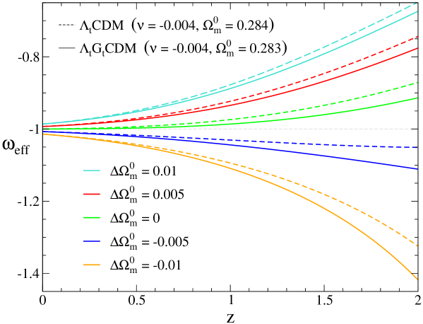
Figure 1: The behavior of the effective EoS function $\omega_{\rm eff}(z)$ for the two running vacuum models. In each case, $\Omega_{m}^{0}$ corresponds to the central value obtained in our fit (cf. Sect. 6) whereas the value of $\nu$ is in the lower limit of the 1$\sigma$ range. For fixed $\nu=-0.004$, and different values and signs of $\Delta\Omega_{m}$, the effective EoS behavior of both running models appears as significantly different from the $\Lambda$CDM prediction ($\omega_{\Lambda}=-1$). Indeed, the effective EoS of the running $\Lambda$ models is seen to present quintessence- or phantom-like behavior, depending on the values of the parameters.

It is remarkable to note that in all time-dependent vacuum models of the form (2), a value $z=z^{*}$ always exists for which the effective EoS $\omega_{\rm eff}(z)$ crosses the phantom divide $\omega_{\rm eff}(z^{*})=-1$, see [12] for the general proof of this statement. For the models under consideration we can easily check that it is so. This is particularly simple if we look at equation (60). For, as $\Omega_{m}^{0}$ and $\hat{\Omega}_{m}^{0}$ must be very close, and $g(z)$ is a slowly monotonous function, the effective EoS crosses the phantom divide at some point $z^{*}$ characterized by the condition $g(z^{*})\Omega_{m}^{0}=\hat{\Omega}_{m}^{0}$. Whether the crossing point $z^{*}$ is in the past or in the future, it will also depend on the sign of $\Delta\Omega_{m}^{0}$ and the value of $\nu$. Clearly, for $\Delta\Omega_{m}^{0}=0$ the crossing is exactly at $z^{*}=0$ since $g(0)=1$. Similarly, it is easy to see that, for $z\to 0$, equation (61) renders $\omega_{\rm eff}^{\Lambda}\to-1$ for $\Delta\Omega_{m}^{0}=0$, whereas if $\Delta\Omega_{m}^{0}>0$ or $\Delta\Omega_{m}^{0}<0$ the behavior is $\omega_{\rm eff}^{\Lambda}\gtrsim-1$ (quintessence-like) or $\omega_{\rm eff}^{\Lambda}\lesssim-1$ (phantom-like) respectively. Furthermore, for both models one can easily show that, if $\Delta\Omega_{m}^{0}=0$, the quintessence/phantom-like behavior at points $z$ near our time is completely controlled by the sign of $\nu$. Indeed, expanding the above expressions in the aforementioned conditions and for small $\nu$, we meet:

$$\omega_{\rm eff}^{\Lambda G}(z) = -1-3\,\nu\frac{\Omega_{m}^{0}}{\Omega_{\Lambda}^{0}}\,(1+z)^{3}\,\ln\left(\Omega_{m}^{0}(1+z)^{3}+\Omega_{\Lambda}^{0}\right)+{\cal O}(\nu^{2})\,,$$ (62)

$$\omega_{\rm eff}^{\Lambda}(z) = -1-3\,\nu\frac{\Omega_{m}^{0}}{\Omega_{\Lambda}^{0}}\,(1+z)^{3}\,\ln(1+z)+{\cal O}(\nu^{2})\,.$$ (63)

These two equations are very similar, but not quite. Nevertheless we find once more that both running models share the property $\omega_{\rm eff}=-1$ at $z=0$. Furthermore, for both running models we also learn that, if $\Delta\Omega_{m}^{0}=0$, the cases $\nu<0$ or $\nu>0$ amount to quintessence-like or phantom-like behaviors respectively. For fixed $\nu$, the quintessence-like or phantom-like behavior can also be modulated by the sign of $\Delta\Omega_{m}$. Some numerical examples are considered in Fig. 1, where the crossing is in the future, except for the cases $\Delta\Omega_{m}^{0}=0$ in which the crossing is at $z=0$ (i.e. precisely at our time).

The previous discussion clearly illustrates, with the help of the two non-trivial running models $\Lambda_{t}G_{t}$CDM and $\Lambda_{t}$CDM discussed in the previous sections, that a generic cosmological model (2) with time-varying vacuum energy generally leads, when described in the DE picture (i.e. as if it consisted of a cosmological self-conserved DE fluid at constant $G$), to a crossing of the phantom divide. Thus it may provide a natural explanation for the observational data, which still admit a tilt in the phantom domain [3], or it may simply explain the apparent quintessence-like behavior, despite there is no fundamental quintessence or phantom field in our framework. In fact, remember that the original CC picture for both models is just a time-varying vacuum model with or without interaction with matter.

In the next section, we confront these running models with the observational data on SNIa, CMB and BAO. As we will see, for values of $\nu$ sufficiently large within the 1$\sigma$ range of our fits, both models predict a cluster redshift distribution that differs noticeably from the $\Lambda$CDM expectations. For such values of $\nu$, the EoS function of our models should also be easily distinguishable from the $\Lambda$CDM value, $\omega_{\Lambda}=-1$, even in the simplest $\Delta\Omega_{m}^{0}=0$ case. We refer once more to Fig. 1, where we have plotted the EoS functions (60) and (61). For large redshifts ($z\sim 1.5-2$) it is even conceivable that the quality of the data provided by forthcoming SNIa experiments could be enough so as to discriminate between both running cosmological models. A combined analysis of clusters and the dark energy EoS could be a most effective strategy to put our models to the test.

6 Confronting the running vacuum models with the latest observations

In this section, we briefly present the basic observational samples and data statistical analysis that will be adopted to constrain the “running” models presented in the previous sections. First of all, we use the Constitution set of 397 type Ia supernovae of Hicken et al. [2]. In order to avoid possible problems related with the local bulk flow, we use a subsample of 366 SNIa, excluding those with $z<0.02$. The corresponding $\chi^{2}_{\rm SNIa}$ function, to be minimized, is:

$$\chi^{2}_{\rm SNIa}({\bf p})=\sum_{i=1}^{366}\left[\frac{{\cal\mu}^{\rm th}(a_{i},{\bf p})-{\cal\mu}^{\rm obs}(a_{i})}{\sigma_{i}}\right]^{2}\;,$$ (64)

where $a_{i}=(1+z_{i})^{-1}$ is the observed scale factor of the Universe for each data, $z_{i}$ is the observed redshift, ${\cal\mu}$ is the distance modulus ${\cal\mu}=m-M=5{\rm log}d_{L}+25$ and $d_{L}(a,{\bf p})$ is the luminosity distance:

$$d_{L}(a,{\bf p})=\frac{c}{a}\int_{a}^{1}\frac{{\rm d}a^{\prime}}{a^{\prime 2}H(a^{\prime})}\;,$$ (65)

with $c$ the speed of light and ${\bf p}$ a vector containing the cosmological parameters (i.e., $\Omega_{m}^{0},\nu$) that we wish to fit for. The previous formula applies only for spatially flat universes, which we are assuming throughout.

On the other hand, we consider the baryonic acoustic oscillations (BAOs), which are produced by pressure (acoustic) waves in the photon-baryon plasma of the early universe, as a result of the existence of dark matter overdensities. Evidence of this excess has been found in the clustering properties of the SDSS galaxies (see [55], [56]) and it provides a “standard ruler” we can employ to constrain dark energy models. In this work we use the newest results of Percival et al. [56], $r_{s}(z_{d})/D_{\rm V}(z_{\star})=0.1390\pm 0.0037$ (see also [57]). Note that $r_{s}$ is the comoving sound horizon size at the baryon drag epoch $z_{d}$, $D_{V}(z)$ is the effective distance measure [55] and $z_{\star}=0.275$. Of course, the quantities $(r_{s},D_{\rm V})$ can be defined analytically. In particular, $r_{s}$ is given by:

$$r_{s}(z_{d})=\frac{c}{\sqrt{3}}\int_{0}^{a_{d}}\frac{da}{a^{2}H(a)\sqrt{1+(3\Omega_{b}^{0}/4\Omega_{\gamma}^{0})a}}\;,$$ (66)

where $a_{d}=(1+z_{d})^{-1}$ and $\Omega_{b}^{0}h^{2}\simeq 0.02263$. In this context, the effective distance is (see [55]):

$$D_{\rm V}(z)\equiv\left[(1+z)^{2}D_{A}^{2}(z)\frac{cz}{H(z)}\right]^{1/3}\;,$$ (67)

where $D_{A}(z)=(1+z)^{-2}d_{L}(z,{\bf p})$ is the angular diameter distance. Therefore, the corresponding $\chi^{2}_{\rm BAO}$ function is simply written as:

$$\chi^{2}_{\rm BAO}({\bf p})=\frac{\left[\frac{r_{s}(z_{d})}{D_{\rm V}(z_{\star})}({\bf p})-0.1390\right]^{2}}{0.0037^{2}}\;.$$ (68)

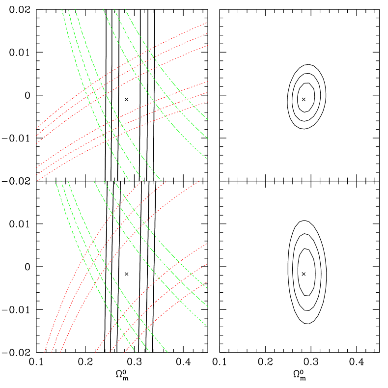
Figure 2: Upper Panel: Likelihood contours (for $-2{\rm ln}{\cal L}/{\cal L}_{\rm max}$ equal to 2.30, 6.16 and 11.81, corresponding to 1$\sigma$, 2$\sigma$ and $3\sigma$ confidence levels) in the $(\Omega_{m}^{0},\nu)$ plane for the $\Lambda_{t}G_{t}$CDM model. The left panel shows the contours based on the SNIa data (thick solid black lines), BAOs (dotted-red lines) and CMB shift parameter (dashed-green lines). In the right panel we show the corresponding contours based on the joint statistical analysis (SNIa+BAO+CMB data). Lower Panel: Similar likelihood contours for the $\Lambda_{t}$CDM model.

Finally, a very accurate and deep geometrical probe of dark energy is the angular scale of the sound horizon at the last scattering surface, as encoded in the location $l_{1}^{TT}$ of the first peak of the Cosmic Microwave Background (CMB) temperature perturbation spectrum. This probe is described by the CMB shift parameter [59, 60], defined as:

$$R=\sqrt{\Omega_{m}}\int_{a_{ls}}^{1}\frac{da}{a^{2}E(a)}$$ (69)

The measured shift parameter according to the WMAP 7-years data [3] is $R=1.726\pm 0.018$ at $z_{ls}=1091.36$ [or $a_{ls}=(1+z_{ls})^{-1}\simeq 9.154\times 10^{-4}$]. In this case, the $\chi^{2}_{\rm cmb}$ function is given by:

$$\chi^{2}_{\rm cmb}({\bf p})=\frac{[R({\bf p})-1.726]^{2}}{0.018^{2}}\;.$$ (70)

Note that the measured CMB shift parameter is somewhat model dependent, but mainly for models that include massive neutrinos or those with a strongly varying equation of state parameter (which is not our case). For a detailed discussion of the shift parameter as a cosmological probe, see [61].

In order to place tighter constraints on the corresponding parameter space of our model, the probes described above must be combined through a joint likelihood analysis, given by the product of the individual likelihoods according to:

$${\cal L}_{tot}({\bf p})={\cal L}_{\rm SNIa}\times{\cal L}_{\rm BAO}\times{\cal L}_{\rm cmb}\;,$$ (71)

which translates in an addition for the joint $\chi^{2}$ function:

$$\chi^{2}_{tot}({\bf p})=\chi^{2}_{\rm SNIa}+\chi^{2}_{\rm BAO}+\chi^{2}_{\rm cmb}\;.$$ (72)

In our $\chi^{2}$ minimization procedure, we use the following range and steps of the fitted parameters: $\Omega_{m}^{0}\in[0.1,1]$ in steps of 0.001 and $\nu\in[-0.02,0.02]$ in steps of $10^{-4}$.

In Figure 2 we present the results of our analysis for the $\Lambda_{t}G_{t}$CDM (upper panel) and the $\Lambda_{t}$CDM (lower panel) models. The left plots in that figure show the 1$\sigma$, 2$\sigma$ and $3\sigma$ confidence levels in the $(\Omega_{m}^{0},\nu)$ plane, with the SNIa-based results indicated by thick solid lines, the BAO results by dotted - red lines and those based on the CMB shift parameter by dashed -green lines. Using the SNIa data alone it is evident that although the $\Omega_{m}^{0}$ parameter is tightly constrained ($\simeq 0.284$), the $\nu$ parameter remains completely unconstrained. As can be seen in the right plots of Figure 2, the above degeneracy is broken when using the joint likelihood analysis, involving all the cosmological data. For the $\Lambda_{t}G_{t}$CDM we find that the overall likelihood function peaks at $\Omega_{m}^{0}=0.283^{+0.012}_{-0.013}$ and $\nu=-0.001\pm 0.0032$ with $\chi_{tot}^{2}(\Omega_{m}^{0},\nu)\simeq 439.36$ for $366$ degrees of freedom.

On the other hand, for the $\Lambda_{t}$CDM model the best fit parameters are: $\Omega_{m}^{0}=0.284^{+0.011}_{-0.014}$ and $\nu=-0.0017^{+0.0051}_{-0.0043}$ with $\chi_{tot}^{2}(\Omega_{m}^{0},\nu)/dof\simeq 439.34/366$. Finally, for the usual $\Lambda$ cosmology ($\nu=0$ and $G=G_{0}$) we find that the overall likelihood function peaks at $\Omega_{m}^{0}=0.284\pm 0.012$ with $\chi_{tot}^{2}(\Omega_{m}^{0})/dof\simeq 439.61/367$. We remark that although for both running models the best fit value for the $\nu$ parameter is negative , its $1\sigma$ range includes both positive and negative $\nu$ values and encompasses quite a wide segment. For instance, for the $\Lambda_{t}G_{t}$CDM model the 1$\sigma$ range is roughly $[-0.004,0.002]$. It is worth mentioning that this range of values is in the same ballpark as the bounds obtained for $\nu$ from the normalization of the spectrum amplitude and from primordial nucleosynthesis [45].

To end this section, let us mention that we have checked that using the earlier BAO results of Eisenstein et al. [55] does not change significantly the previously presented constraints.

7 Halo abundances and their evolution in dark energy models

In an attempt to define observational criteria that will enable us to identify the realistic variants of the concordance $\Lambda$CDM cosmology and distinguish among the different $\Lambda(t)$ models, we derive and compare their theoretically predicted cluster-size halo redshift distributions.

The formalism to compute the fraction of matter in the universe that has formed bounded structures and its redshift distribution was developed in 1974 by Press and Schechter [62] (hereafter PSc). In their approach, the primordial density fluctuation for a given mass $M$ of the dark matter fluid is described by a random Gaussian field. One introduces a function, ${\cal F}(M,z)$, representing the fraction of the universe that has collapsed by the redshift $z$ in halos above some mass $M$. With this function one may estimate the (comoving) number density of halos, $n(M,z)$, with masses within the range $(M,M+\delta M)$:

$$n(M,z)dM=\frac{\partial{\cal F}(M,z)}{\partial M}\frac{{\bar{\rho}}}{M}dM.$$ (73)

This expression can be rewritten as follows:

$$n(M,z)dM = -\frac{\bar{\rho}}{M}\left(\frac{1}{\sigma}\frac{d\sigma}{dM}\right)f_{\rm PSc}(\sigma)dM=\frac{\bar{\rho}}{M}\frac{d{\rm\ln}\sigma^{-1}}{dM}f_{\rm PSc}(\sigma)dM,$$ (74)

where $f_{\rm PSc}(\sigma)=\sqrt{2/\pi}(\delta_{c}/\sigma)\exp(-\delta_{c}^{2}/2\sigma^{2})$, $\delta_{c}$ is the linearly extrapolated density threshold above which structures collapse [63] (see Appendix  A for more details), while $\sigma^{2}(M,z)$ is the mass variance of the smoothed linear density field, which depends on the redshift $z$ at which the halos are identified. It is given in Fourier space by:

$$\sigma^{2}(M,z)=\frac{D^{2}(z)}{2\pi^{2}}\int_{0}^{\infty}k^{2}P(k)W^{2}(kR)dk\;,$$ (75)

where $D(z)$ is the growth factor of perturbations, $P(k)$ is the power-spectrum of the linear density field, and $W(kR)=3({\rm sin}kR-kR{\rm cos}kR)/(kR)^{3}$ is the top-hat smoothing function, which contains on average a mass $M$ within a radius $R=(3M/4\pi\bar{\rho})^{1/3}$ and $\bar{\rho}=2.78\times 10^{11}\Omega_{m}^{0}h^{2}M_{\odot}$Mpc^-3. We use the CDM power spectrum:

$$P(k)=P_{0}k^{n}T^{2}(\Omega_{m}^{0},k)\,,$$ (76)

with $T(\Omega_{m}^{0},k)$ the BBKS transfer function [64]:

$$T(\Omega_{m}^{0},k) = \frac{\ln(1+2.34q)}{2.34q}\Big{[}1+3.89q+(16.1q)^{2}+\,(5.46q)^{3}+(6.71q)^{4}\Big{]}^{-1/4}\,,$$

$$q=q(k) \equiv \frac{k}{h\Gamma}\,.$$ (77)

Here $\Gamma$ is the shape parameter, according to [65], provided by the 7-year WMAP results [3], in combination with the model fitted $\Omega_{m}$ values of section 6. Note that in this approach all the mass is locked inside halos, according to the normalization constraint:

$$\int_{-\infty}^{+\infty}f_{\rm PSc}(\sigma)d{\rm\ln}\sigma^{-1}=1\;.$$ (78)

It is traditional to parametrize the mass variance in terms of $\sigma_{8}$, the rms mass fluctuation amplitude on scales of $R_{8}=8\;h^{-1}$ Mpc at redshift $z=0$ [$\sigma_{8}\equiv\sigma_{8}(0)$], so that we have:

$$\sigma^{2}(M,z)=\sigma^{2}_{8}(z)\frac{\int_{0}^{\infty}k^{n+2}T^{2}(\Omega_{m}^{0},k)W^{2}(kR)dk}{\int_{0}^{\infty}k^{n+2}T^{2}(\Omega_{m}^{0},k)W^{2}(kR_{8})dk}\,,$$ (79)

where

$$\sigma_{8}(z)=\sigma_{8}\frac{D(z)}{D(0)}\;.$$ (80)

Although the previously described Press-Schechter formalism was shown to provide a good first approximation to the halo mass function obtained by numerical simulations, it was later found to over-predict/under-predict the number of low/high mass halos at the present epoch [66, 67]. More recently, a large number of works have provided better fitting functions for $f(\sigma)$, some of them based on a phenomenological approach. In the present treatment, we adopt the one proposed by Reed et al. [68]:

$$f(\sigma,n_{\rm eff})=A\sqrt{{2b\over\pi}}\left[1+\left({\sigma^{2}\over b\delta_{c}^{2}}\right)^{p}+0.6G_{1}+0.4G_{2}\right]{\delta_{c}\over\sigma}\exp\left[-{cb\delta_{c}^{2}\over 2\sigma^{2}}-{0.03\over(n_{\rm eff}+3)^{2}}\left({\delta_{c}\over\sigma}\right)^{0.6}\right],\\$$

where $A=0.3222,\,p=0.3,\,b=0.707,\,c=1.08$, while $G_{1},\,G_{2}$ and $n_{\rm eff}$, the slope of the non-linear power-spectrum at the halo scale, are given by:

$$G_{1}=\exp\left[-{{(\ln\sigma^{-1}-0.4)^{2}}\over{2(0.6)^{2}}}\right],\;G_{2}=\exp\left[-{{(\ln\sigma^{-1}-0.75)^{2}}\over{2(0.2)^{2}}}\right],\;n_{\rm eff}=6{{\rm d}\ln\sigma^{-1}\over{\rm d}\ln M\phantom{+}}-3.$$ (81)

7.1 Collapse threshold and mass variance of the running vacuum models

In order to compare the mass function predictions for the different vacuum models, it is imperative to use for each model the appropriate value of $\delta_{c}$ and $\sigma_{8}$. Indeed, the way in which dark energy (time-varying vacuum energy, in our case) affects the formation of gravitationally bound systems (clusters of galaxies) is a crucial question that has received a lot of attention in the literature. Three distinct scenarios (with increasing level of difficulty in the theoretical treatment) can be considered, to wit: (i) dark energy remains homogeneous and only matter virializes; (ii) dark energy may cluster but only matter virializes; and (iii) dark energy may also cluster and the whole system (matter and dark energy) virializes. The first scenario has been widely used in the literature, probably because it is the simplest one  [35, 36, 37, 38, 39]. In the present paper, we will consider just this canonical scenario when dealing with the $\Lambda_{t}$CDM model. For the full running FLRW model (or $\Lambda_{t}G_{t}$CDM model), however, which is the main object of the present study, we will go a bit deeper and we shall treat the gravitational collapse within the framework of the second scenario (in which $\delta G$ and $\delta_{\Lambda}$ are both non-vanishing and only matter virializes). Then, in the Appendix  A we shall compare these results for the $\Lambda_{t}G_{t}$CDM model within scenario (ii) to those obtained within the canonical scenario (i), for which $\delta G=\delta_{\Lambda}=0$  .

It is well known that for the usual $\Lambda$ cosmology $\delta_{c}\simeq 1.675$, while Weinberg & Kamionkowski [34] provide an accurate fitting formula to estimate $\delta_{c}$ for DE models with constant EoS parameter. It should furthermore be noted that such a formula is, in principle, only applicable to “conventional” DE models, i.e. models with self-conserved matter and DE densities and constant $G$. Although these conditions are not satisfied by our running vacuum models, one can show [38, 40] that the $\delta_{c}$ values for a large family of dark energy models with a time-varying EoS parameter can be well approximated using the previously discussed fitting formula, as long as the EoS parameter is not very different from -1 near the present epoch. This is indeed the case for our models, as shown in Fig. 1. In spite of this prognosis, we will nevertheless carefully compute the value of $\delta_{c}$ within our vacuum models, following the prescriptions given in [38] (cf. Sect. 2.1 in that reference) and [33]. Starting from a Newtonian formalism, we derive a non-linear second-order differential equation for the evolution of the matter perturbations in our vacuum models from which we compute $\delta_{c}(z)$, and in particular $\delta_{c}\equiv\delta_{c}(0)$ (cf. Appendix  A for the calculational details and methodology). The resulting values are listed in Table 1. As an example, in the case of the $\Lambda_{t}G_{t}$CDM model, for $\Omega_{m}^{0}=0.283$ and $\nu=-0.001$ we find $\delta_{c}\simeq 1.677$, pretty close to the $\Lambda$CDM value ($\simeq 1.675$). On the other hand, for the $\Lambda_{t}$CDM model ($\Omega_{m}^{0}=0.284$, $\nu=-0.0017$) we find a bit larger value, $\delta_{c}\simeq 1.685$. In all cases, however, the differences with respect to the $\Lambda$CDM value are at the few per mil level only. This is in agreement with the expectations for our models, and it is exactly the same that happens in other models [38, 40].

The relevant $\sigma_{8}$ value for the different “running” vacuum models can be estimated by scaling the present time $\Lambda$CDM value ($\sigma_{8,\Lambda}$) using equation (75). In general, for any DE model, equation (75) takes the form:

$$\sigma_{\rm 8}=\sigma_{8,\Lambda}\frac{D(0)}{D_{\Lambda}(0)}\left[\frac{P_{0}\int_{0}^{\infty}k^{n+2}T^{2}(\Omega_{m}^{0},k)W^{2}(kR_{8})dk}{P_{\Lambda,0}\int_{0}^{\infty}k^{n+2}T^{2}(\Omega_{m,\Lambda}^{0},k)W^{2}(kR_{8})dk}\right]^{1/2}\,,$$ (82)

where $P_{0}/P_{\Lambda,0}=(\Omega_{m,\Lambda}^{0}/\Omega_{m}^{0})^{2}$.

Therefore, using the observationally determined value for $\sigma_{8,\Lambda}$, we can easily derive the corresponding $\sigma_{\rm 8}$ value for any of the time-varying vacuum models. Indeed, the joint WMAP7+BAO+$H_{0}$ analysis of Komatsu et al. [3] resulted in a value of $\sigma_{8,\Lambda}=0.811$. This value is in quite good agreement with that provided by a variety of different methods; for example, an analysis based on cluster abundances gave the degenerate combination: $\sigma_{8,\Lambda}=\left(0.83\pm 0.03\right)(\Omega_{m}^{0}/0.25)^{-0.41}$ [69]. The weak-lensing analysis of Fu et al. [70] provided $\sigma_{8,\Lambda}=\left(0.837\pm 0.084\right)(\Omega_{m}^{0}/0.25)^{-0.53}$, while two recent studies based on a joint analysis of the large-scale clustering of red SDSS galaxies, CMB, SNIa and BAO data resulted in: $\sigma_{8,\Lambda}\simeq 0.8\pm 0.02$ (for $\Omega^{0}_{m}\simeq 0.26$) [71, 72]. The only method that provides discrepant results is that based on galaxy or cluster peculiar velocities [73, 74].

Finally, inserting the Komatsu et al. [3] $\sigma_{8,\Lambda}$ value in equation (82) we can estimate the corresponding $\sigma_{\rm 8}$ values for our models. These values will be used in the mass function analysis and are listed in Table 1.

7.2 Halo mass function & number counts of the running vacuum models

We now move to our results. Given the halo mass function from Eq. (74) we can derive an observable quantity which is the redshift distribution of clusters, ${\cal N}(z)$, within some determined mass range, say $M_{1}\leq M\leq M_{2}$. This can be estimated by integrating the expected differential halo mass function, $n(M,z)$, with respect to mass, according to:

$${\cal N}(z)=\frac{dV}{dz}\;\int_{M_{1}}^{M_{2}}n(M,z)dM,$$ (83)

where $dV/dz$ is the comoving volume element, which in a flat universe takes the form:

$$\frac{dV}{dz}=4\pi r^{2}(z)\frac{dr(z)}{dz},$$ (84)

with $r(z)$ denoting the comoving radial distance out to redshift $z$:

$$r(z)=\frac{c}{H_{0}}\int_{0}^{z}\frac{dz^{\prime}}{E(z^{\prime})}.$$ (85)

In the upper panel of Fig. 3, we show the theoretically expected redshift distribution, ${\cal N}(z)$, for cluster-size halos, ie., $M_{1}=10^{13.4}\;h^{-1}M_{\odot}$ and $M_{2}=10^{16}\;h^{-1}M_{\odot}$ for the $\Lambda_{t}G_{t}$CDM, $\Lambda_{t}$CDM and $\Lambda$CDM models, using the best-fit values for the $\Omega_{m}^{0}$ and $\nu$ parameters provided in section 6 (also indicated in Table 1). In the lower panel we show the relative differences of the two running models with respect to the concordance $\Lambda$CDM model. The different models are characterized by the symbols and line types presented in Table 1.

It is evident that, for the central fit values of the $\nu$ parameter, the $\Lambda_{t}$CDM is the only model which shows significant differences with respect to the concordance $\Lambda$CDM model, producing a larger number of cluster-size halos at any given redshift. As for the $\Lambda_{t}G_{t}$CDM model, although it also produces larger numbers of halos than the $\Lambda$CDM model, the differences are minimal. For instance, for $2<z<3$ the $\Lambda_{t}$CDM model presents $\delta{\cal N}/{\cal N}\sim 0.47$, whereas in the $\Lambda_{t}G_{t}$CDM case the corresponding value amounts to only $\sim 0.06$.

However, in order to assess whether it is possible to observationally discriminate between the different vacuum models, we need to concentrate on a more significant model comparison by deriving the expected halo redshift distributions in the context of realistic future cluster surveys.

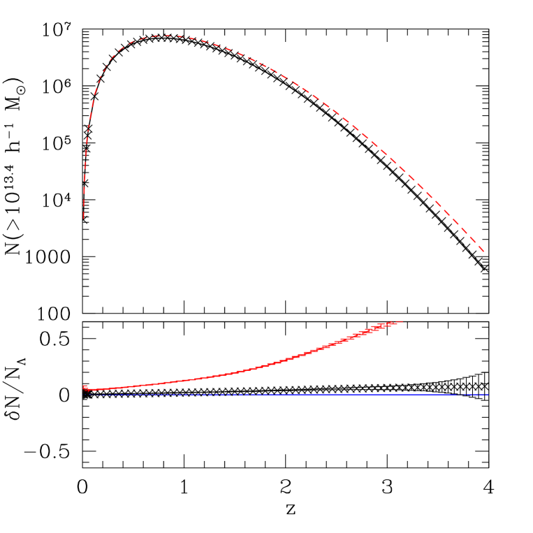
Figure 3: The theoretical redshift distribution of $M\raise-3.0pt\hbox{\hbox to0.0pt{\hbox{$\sim$}\hss}\raise 4.0pt\hbox{$>$}\ }10^{13.4}h^{-1}M_{\odot}$ clusters (upper panel) for the different vacuum models and the corresponding fractional difference (lower panel) between the running models and the reference $\Lambda$CDM model. The running models are plotted for the central fit values of the $\nu$ parameter, $\nu=-0.0017$ (red dashed line) for the $\Lambda_{t}$CDM and $\nu=-0.001$ (black crosses) for the $\Lambda_{t}G_{t}$CDM. The full list of input parameters, corresponding to the central fit values, as well as the symbols or line-types characterizing the different models, are shown in Table 1. Error bars are 2$\sigma$ Poisson uncertainties.

Two of these realistic future surveys are:

(a) The eROSITA satellite X-ray survey, with a flux limit of $f_{\rm lim}=3.3\times 10^{-14}$ ergs s^-1 cm^-2, at the energy band 0.5-5 keV and covering $\sim 20000$ deg² of the sky.

(b) The South Pole Telescope (SPT) Sunyaev-Zeldovich (SZ) survey, with a limiting flux density at $\nu_{0}=150$ GHz of $f_{\nu_{0},{\rm lim}}=5$ mJy and a sky coverage of $\sim 4000$ deg².

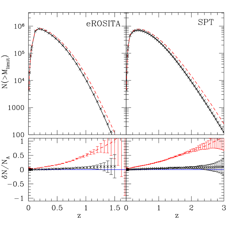
Figure 4: The expected cluster redshift distribution, over the whole sky, of the two running vacuum models for the case of the two future cluster surveys eROSITA and SPT (upper panels), and the corresponding fractional difference with respect to the reference $\Lambda$CDM model (lower panels). The input parameters, corresponding to the central fit values, as well as the symbols or line-types characterizing the different models are shown in Table 1.

To realize the predictions of the first survey we use the relation between halo mass and bolometric X-ray luminosity, as a function of redshift, provided in [75]:

$$L(M,z)=3.087\times 10^{44}\left[\frac{ME(z)}{10^{15}h^{-1}M_{\odot}}\right]^{1.554}h^{-2}\;{\rm ergs^{-1}}\;.$$ (86)

The limiting halo mass that can be observed at redshift $z$ is then found by inserting in the above equation the limiting luminosity, given by: $L=4\pi d_{L}^{2}f_{\rm lim}$c_b, with $d_{L}$ the luminosity distance corresponding to the redshift $z$ and c_b the band correction, necessary to convert the bolometric luminosity of Eq. (86) to the 0.5-5 keV band of eROSITA. We estimate this correction by assuming a Raymond-Smith [76] plasma model with a metallicity of 0.4$Z_{\odot}$, a typical cluster temperature of $\sim 4$ keV and a Galactic absorption column density of $n_{H}=10^{21}$ cm^-2.

The predictions of the second survey can be realized using again the relation between limiting flux and halo mass from [75]:

$$f_{\nu_{0},{\rm lim}}=\frac{2.592\times 10^{8}{\rm mJy}}{d_{A}^{2}(z)}\left(\frac{M}{10^{15}M_{\odot}}\right)^{1.876}E^{2/3}(z)\;$$ (87)

where $d_{A}(z)\equiv d_{L}/(1+z)^{2}$ is the angular diameter distance out to redshift $z$.

In Fig.4 (upper panels) we present the expected redshift distributions above a limiting halo mass, which is $M_{1}\equiv M_{\rm limit}=\max[10^{13.4}h^{-1}M_{\odot},M_{f}]$, with $M_{f}$ corresponding to the mass related to the flux-limit at the different redshifts, estimated by solving Eq. (86) and Eq. (87) for $M$. In the lower panels we present the fractional difference between the two time-varying vacuum models ($\Lambda_{t}$CDM and $\Lambda_{t}G_{t}$CDM) and the $\Lambda$CDM, similarly to Fig.3, but now for the realistic case of the previously mentioned future cluster surveys. The error bars shown correspond to 2$\sigma$ Poisson uncertainties, which however do not include cosmic variance and possible observational systematic uncertainties, that would further increase the relevant variance.

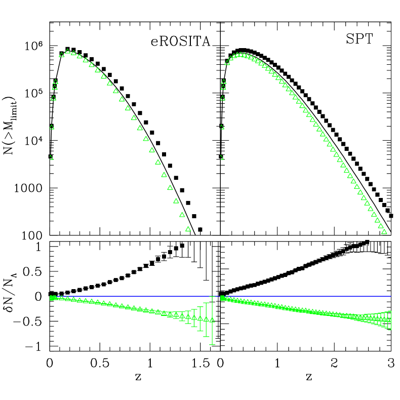
Figure 5: Extension of the analysis presented in Fig. 4, but for the $\Lambda_{t}G_{t}$CDM model only. Once more the theoretical redshift distribution of $M\raise-3.0pt\hbox{\hbox to0.0pt{\hbox{$\sim$}\hss}\raise 4.0pt\hbox{$>$}\ }10^{13.4}h^{-1}M_{\odot}$ clusters in the two future surveys is shown in the upper panel, whereas the corresponding fractional difference with respect to the $\Lambda$CDM model is shown in the lower panel. In this case, we use the limiting values of $\nu$ comprised within the $1\sigma$ range of our fit, namely $\nu=-0.004$ (black squares) and $\nu=+0.002$ (green triangles). See Table 1.

It is evident that the imposed flux limits, together with the scarcity of high-mass halos at large redshifts, induces an abrupt decline of ${\cal N}(z)$ with $z$, especially in the case of the eROSITA X-ray survey (note the shallower redshifts depicted in Fig.4 with respect to Fig.3). Furthermore, in the case of the $\Lambda_{t}$CDM model the uncertainties indicate that we should expect significant and large differences to be measured in both experiments for any redshift $\sim$$>$  0.3-0.4. On the other hand, the deviations of the $\Lambda_{t}G_{t}$CDM model with respect to the concordance model, although significant, are very small (for the central fit values) and thus more difficult to detect.

Model	symbol	$\Omega_{m}^{0}$	$\nu$	$\sigma_{8}$	$\delta_{c}$	($\delta{\cal N}/{\cal N}_{\Lambda})_{\rm eROSITA}$		$(\delta{\cal N}/{\cal N}_{\Lambda})_{\rm SPT}$
						$z<0.2$	$0.5\leq z<1$	$z<0.2$	$1\leq z<2$
$\Lambda$CDM	black line	0.284	0	0.811	1.675	0.00	0.00	0.00	0.00
$\Lambda_{t}G_{t}$CDM	black crosses	0.283	-0.001	0.818	1.677	0.01	0.04	0.01	0.05
$\Lambda_{t}$CDM	red dashed line	0.284	-0.0017	0.840	1.685	0.05	0.25	0.06	0.36
$\Lambda_{t}G_{t}$CDM	black squares	0.283	-0.004	0.853	1.683	0.06	0.32	0.07	0.45
$\Lambda_{t}G_{t}$CDM	green triangles	0.283	0.002	0.786	1.671	-0.05	-0.18	-0.05	-0.23

Table 1: Numerical results. The $1^{st}$ column indicates the dark energy model. The $2^{nd}$ column shows the symbols or lines used to represent the different models in Figs. 3, 4 and 5. The $3^{rd}$, $4^{th}$ and $5^{th}$ columns list the central values of the input fitted cosmological parameters (first three rows, one for each model being considered) and their limiting $1\sigma$ values (last two rows, only for the $\Lambda_{t}G_{t}$CDM model) obtained by using the SNIa+BAO+CMB data (cf. section 6). The procedure to compute the critical overdensity $\delta_{c}$ for each model ($6^{th}$ column) is explained in Appendix  A. The remaining columns present the overall, within the indicated redshift bins, fractional relative difference [$\delta\mathcal{N}/\mathcal{N}_{\Lambda}\equiv(\mathcal{N}-\mathcal{N}_{\Lambda})/\mathcal{N}_{\Lambda}$] between the cluster abundances predicted by the time varying vacuum models and by the $\Lambda$CDM cosmology, for the two future cluster surveys discussed in the text. No errors are shown since the 2$\sigma$ Poisson uncertainties are less than $10^{-2}$.

Let us stress that the previous analysis of the cluster-size halo redshift distribution has focused on the central values of our fits to the SNIa+BAO+CMB data (cf. section 6). However, there is no compelling reason to prefer the central values to any other value within the 1$\sigma$ contour. This observation is particularly important when the dispersion turns out to be considerably large in that range. As we saw in section 6, the $1\sigma$ range of the fitted $\nu$ parameter for both running models is indeed quite large and includes both positive and negative values. In particular, for the $\Lambda_{t}G_{t}$CDM model we have obtained $\nu\in[-0.004,0.002]$. This model deserves special attention in that, in contrast to the $\Lambda_{t}$CDM, the time evolution of the vacuum energy density is compatible with matter conservation (a feature that shares with the standard $\Lambda$CDM model). It is therefore worthwhile to perform a more exhaustive investigation of the cluster halo redshift distribution for this model within the limits of the $1\sigma$ range, so as to check if the predicted deviations with respect to the $\Lambda$CDM can be significant. We display the results of this extended analysis in Fig. 5, where we show, following a pattern entirely similar to that in Fig. 4, the expectations of the $\Lambda_{t}G_{t}$CDM model for the limiting $\nu$ values in its $1\sigma$ range [ie., $\nu=-0.004$ (black squares) and $\nu=0.002$ (open triangles)]. It is evident that, in this case, the predicted redshift distribution of clusters, ${\cal N}(z)$, for the $\Lambda_{t}G_{t}$CDM model does show significantly larger, and potentially measurable, differences ($\sim 50\%$) with respect to the concordance $\Lambda$CDM model, even at moderate redshifts.

In Table 1, we show a more compact presentation of our results, including the relative fractional difference between the “running” vacuum models and the $\Lambda$CDM model, in two characteristic redshift bins, and for both future surveys under consideration (eROSITA and SPT). The first redshift bin corresponds to the local universe ($z\raise-3.0pt\hbox{\hbox to0.0pt{\hbox{$\sim$}\hss}\raise 4.0pt\hbox{$<$}\ }0.2$) and it is shown in order to allow us to judge whether the existing cluster samples could be used to discriminate among the different models. It is evident that in the local range $z\raise-3.0pt\hbox{\hbox to0.0pt{\hbox{$\sim$}\hss}\raise 4.0pt\hbox{$<$}\ }0.2$, although there are deviations among the models, their amplitude is very small and it will be rather difficult to detect them unambiguously. However, at larger redshifts, the amplitude of the deviations is such that it should be relatively straightforward to distinguish among the different models.

To conclude, in view of the results of our analysis of the cluster halo redshift distribution, ${\cal N}(z)$, presented in Figures 4, 5 and Table 1, we can say that both running models show large and significant differences with respect to the $\Lambda$CDM within the 1$\sigma$ range of the fitted values of the fundamental parameter $\nu$ of these models. We have demonstrated that these deviations could be measured for the two future cluster surveys considered in our study (eROSITA and SPT) provided we focus on sufficiently high cosmological redshifts $z\raise-3.0pt\hbox{\hbox to0.0pt{\hbox{$\sim$}\hss}\raise 4.0pt\hbox{$>$}\ }0.3$, therefore outside the local domain. In practice, eROSITA will be most efficient in the redshift range $0.3\lesssim z\lesssim 1.2$ whereas SPT in the wider segment $0.3\lesssim z\lesssim 2.2$, where in both cases the upper limit on $z$ is determined by the sharp decrease in the cluster number counts and the corresponding larger statistical error.

Let us finally point out that, had we used the same rms mass fluctuation normalization for both time-varying vacuum models, i.e., $\sigma_{\rm 8}=\sigma_{8,\Lambda}$ (as in [31]), we would have found that none of the time-varying vacuum models could be distinguished from the reference $\Lambda$CDM model at a significant level. This implies that the value of $\sigma_{8}$ plays also a fundamental role in these kind of studies, especially when the models have similar Hubble functions and perturbation growing modes, as it is the case in the presently studied time-varying vacuum models. Therefore, our including the computation of the value of $\sigma_{8}$ for each of the models under consideration has been an important feature of our study, and illustrates the general need to follow this practice for other cosmological models.

8 Conclusions

In this work, we have analyzed the observational status of the “running FLRW model” (denoted by $\Lambda_{t}G_{t}$CDM), i.e. the cosmological model characterized by the vacuum energy density evolving quadratically with the expansion rate, $\rho_{\Lambda}(H)=n_{0}+n_{2}\,H^{2}$ (with $n_{0}\neq 0$). The non-vanishing coefficient $n_{2}$ provides the time evolution of the cosmological term, and since it is a dimensional quantity it is conveniently parametrized as $n_{2}=(3\nu/8\pi)\,M_{P}^{2}$, where $\nu$ plays the role of the dimensionless $\beta$-function of the running $\rho_{\Lambda}$. This is particularly clear also from the simultaneous running of the gravitational coupling in this model, which evolves logarithmically with the expansion rate according to $G^{-1}(H)\sim M_{P}^{2}(1+\nu\ln H^{2})$. These two running laws are intimately correlated such that the Bianchi identity is automatically satisfied, as demanded by general covariance. As a result, a nice feature of this model is that matter is locally and covariantly conserved, similarly to the standard $\Lambda$CDM model. It means that, in the $\Lambda_{t}G_{t}$CDM model, there is no decay of vacuum energy into matter or vice versa. This is in contradistinction to a previous version of the model, the running $\Lambda_{t}$CDM model, which was recently confronted with the latest observations in [31]. We have re-analysed this model here, together with the $\Lambda_{t}G_{t}$CDM model, so as to better highlight the similarities as well as the important differences between them. In both running models, $\rho_{\Lambda}(H)$ is varying formally in the same way as a function of $H$, but in the $\Lambda_{t}$CDM model $G$ is strictly constant at the price of permitting a continuous exchange of energy between vacuum and matter.

We have confronted $\Lambda_{t}G_{t}$CDM and $\Lambda_{t}$CDM in the light of the latest high-quality cosmological data from distant type Ia supernovae, baryonic acoustic oscillations and the cosmic microwave background anisotropies. This has allowed us to put a limit on the size of the fundamental parameter $\nu$ controlling the running of the vacuum energy in both models. This parameter also controls the running of the gravitational coupling in the $\Lambda_{t}G_{t}$CDM case, or alternatively the exchange of vacuum energy and matter in the $\Lambda_{t}$CDM model. Despite the fact that the two models are qualitatively quite different, for both of them we find that if $\nu<0$ the formation of structure is reinforced with respect to the $\Lambda$CDM, whereas for $\nu>0$ it is depleted. This is understandable in the sense that, for $\nu<0$, the vacuum energy decreases in the past (it may even become negative) and therefore the formation of structure is favored. In contrast, for $\nu>0$ the vacuum energy becomes larger and positive in the past, preventing the growth of structure.

Although the central fitted $\nu$ values of the two running models are different, in both cases we meet the preferred sign $\nu<0$, with a magnitude of order $|\nu|={\cal O}(10^{-3})$. Furthermore, the corresponding $1\sigma$ ranges are quite consistent among them, especially when one takes into account their relative uncertainty, which is of the same order as the central value, i.e. $|\delta\nu|={\cal O}(10^{-3})$. As a result, both the $\Lambda_{t}$CDM and $\Lambda_{t}G_{t}$CDM models could show significant departures with respect to the $\Lambda$CDM power spectrum within one standard deviation of the fitted values. This fact translates then into a measurable impact on the redshift distribution of cluster-size halos, as we have verified in detail, finding that both running models could lead to very important deviations with respect to the concordance model.

Interestingly enough, the redshift distribution of cluster-size halos will be measured by two future important surveys, one is based on the X-ray eROSITA satellite and the other on the Sunyaev-Zeldovich observations performed by the South Pole Telescope (SPT). Our analysis shows that by sampling $\nu$ within its $1\sigma$ range there is a significant maximal deviation –positive or negative, depending on the sign of $\nu$– in the predicted abundance of clusters with respect to the $\Lambda$CDM, which could amount to an anomaly of $50\%$ or higher at redshifts ranges ($z\gtrsim 0.3$) which should be perfectly accessible to both realistic surveys.

Finally, let us emphasize that both models display an effective equation of state behavior which can mimic both quintessence and phantom dark energy, without of course involving quintessence or phantom scalar fields. It follows that the sole EoS behavior of the running cosmologies can be highly distinctive with respect to the concordance $\Lambda$CDM model and it can also be used to distinguish between the two running models themselves. This strategy should be most efficient upon combining the effective EoS determination with the predicted deviations of the clustering redshift distribution with respect to the $\Lambda$CDM. The upshot of our study is that the “running cosmologies” could provide an alternative and successful version of dynamical dark energy which should be testable in the next generation of cosmological experiments.

Appendix A The critical overdensity in time-varying vacuum models

In this appendix we explain in detail the computation of $\delta_{c}$ (the linearly extrapolated density threshold above which structures collapse) for the RG models we have considered. The quantity $\delta_{c}$ is used for the study of the halo abundances and their evolution in Sect. 7.

The $\Lambda_{t}G_{t}$CDM model:

First we have to derive the second-order differential equation governing the non-linear evolution of the matter perturbations in our model. Using the Newtonian formalism for the cosmological fluid, we start by writing the continuity, Euler and Poisson equations in the matter dominated epoch:

$$\frac{\partial\rho_{m}}{\partial t}+\nabla_{\vec{r}}\cdot(\rho_{m}\vec{v})=0\;,$$ (88)

$$\frac{\partial\vec{v}}{\partial t}+(\vec{v}\cdot\nabla_{\vec{r}})\,\vec{v}+\nabla_{\vec{r}}\,\Phi=0\;,$$ (89)

$$\nabla^{2}\Phi=4\pi G_{\!N}\sum_{i}\rho_{i}(1+3\omega_{i})\;,$$ (90)

where $\vec{v}$ is the total velocity of the co-moving observer in three-space, $\Phi$ is the Newtonian gravitational potential, $\vec{r}$ is the physical coordinate, $G_{\!N}$ is the Newton’s coupling and $\sum_{i}$ runs over all the energy components, in our case non-relativistic matter and the running cosmological constant ($i=m,\,\Lambda$). Finally, $\omega_{i}=p_{i}/\rho_{i}$ is the EoS parameter for each component ($0$ for dust, and $-1$ for the CC, respectively). Let us recall that, within this framework, $G_{\!N}$ and $\rho_{\Lambda}$ depend on time (at the background level). We introduce comoving coordinates $\vec{x}=\vec{r}/a$ and define the perturbations in the following way:

$$\rho_{i}(\vec{x},t) = \bar{\rho}_{i}(t)+\delta\rho_{i}(\vec{x},t)=\bar{\rho}_{i}(t)(1+\delta_{i}(\vec{x},t))\;,$$ (91)

$$\Phi(\vec{x},t) = \Phi_{0}(\vec{x},t)+\phi(\vec{x},t)\;,$$ (92)

$$\vec{v}(\vec{x},t) = a(t)[H(t)\vec{x}+\vec{u}(\vec{x},t)]\;,$$ (93)

$$G_{N}(\vec{x},t) = G(t)+\delta G(\vec{x},t)\;.$$ (94)

Here $H(t)$ is the Hubble function, and $\vec{u}(\vec{x},t)$ is the comoving peculiar velocity. We have introduced also a perturbation for $G_{N}$, equation (94), which is mandatory in order to have a consistent picture in the model under consideration [45]. Furthermore, in view of the corresponding EoS for vacuum and non-relativistic matter, $\delta p_{\Lambda}=-\delta\rho_{\Lambda}$ and $\delta p_{m}=0$. Our next task is to insert Eqs. (91)–(94) into Eqs. (88)–(90). To this end we first use the definition of the gradient with respect to co-moving coordinates, $\vec{\nabla}\equiv\nabla_{\vec{x}}=a(t)\nabla_{\vec{r}}$, and in this way we can express the result as follows:

$$\dot{\delta}_{m}+(1+\delta_{m})\vec{\nabla}\cdot\vec{u} = 0\;,$$ (95)

$$\frac{\partial\vec{u}}{\partial t}+2H\vec{u}+(\vec{u}\cdot\vec{\nabla})\vec{u}+\frac{1}{a^{2}}\vec{\nabla}\phi = 0\;,$$ (96)

$$\nabla^{2}\phi-4\pi Ga^{2}\left(\bar{\rho}_{m}\delta_{m}-2\bar{\rho}_{\Lambda}\delta_{\Lambda}\right)-4\pi a^{2}\delta G\left(\bar{\rho}_{m}-2\bar{\rho}_{\Lambda}\right) = 0\;.$$ (97)

Note that in order to get (95) we have assumed the condition $\vec{\nabla}\delta_{m}=0$, which holds for the spherical collapse of a top-hat distribution [33]. Next we take the divergence of the Euler equation (96) while using the following identity 

$$\vec{\nabla}\cdot[(\vec{u}\cdot\vec{\nabla})\,\vec{u}]=\frac{1}{3}(\vec{\nabla}\cdot\vec{u})^{2}\;,$$ (98)

together with the time derivative of the continuity equation (95). Combining all three equations, we finally obtain the fully non-linear evolution of the matter density contrast:

$$\ddot{\delta}_{m}+2H\dot{\delta}_{m}-\frac{4}{3}\frac{\dot{\delta}_{m}^{2}}{1+\delta_{m}}-4\pi G(1+\delta_{m})\left(\bar{\rho}_{m}\delta_{m}-2\bar{\rho}_{\Lambda}\delta_{\Lambda}\right)-4\pi\delta G(1+\delta_{m})\left(\bar{\rho}_{m}-2\bar{\rho}_{\Lambda}\right)=0\;.$$ (99)

Inserting now Eq. (44) into (99), we are left with:

$$\ddot{\delta}_{m}+2H\dot{\delta}_{m}-\frac{4}{3}\frac{\dot{\delta}_{m}^{2}}{1+\delta_{m}}-4\pi G\bar{\rho}_{m}(1+\delta_{m})\left[\delta_{m}+\frac{\delta G}{G}\right]=0\;.$$ (100)

Changing the independent variable from cosmic time $t$ to the scale factor $a$ through the relation $\partial_{t}=aH\partial_{a}$, equation (100) can be rewritten

$$\delta_{m}^{\prime\prime}+\left(\frac{3}{a}+\frac{H^{\prime}}{H}\right)\delta_{m}^{\prime}-\frac{4}{3}\frac{\delta_{m}^{\prime 2}}{1+\delta_{m}}-\frac{3\tilde{\Omega}_{m}(a)}{2a^{2}}(1+\delta_{m})\left[\delta_{m}+\frac{\delta G}{G}\right]\;,$$ (101)

where $\tilde{\Omega}_{m}(a)$ is defined in (26) and $f^{\prime}=\partial_{a}f$ for any $f$. In the particular case when $G$ is constant there are no perturbations of $G$ in (94) and then equation (101) boils down to Eq. (18) in [38], as it should (see also Eq. (7) in [33]). Indeed, for constant $G$, the relation (26) tells us that $\tilde{\Omega}_{m}(a)=\Omega_{m}(a)/E^{2}(a)=\Omega_{m}^{0}/\left(a^{3}\,E^{2}(a)\right)$. Let us also remark that (101) reduces to

$$\delta_{m}^{\prime\prime}+\left(\frac{3}{a}+\frac{H^{\prime}}{H}\right)\delta_{m}^{\prime}-\frac{3\tilde{\Omega}_{\mathrm{m}}(a)}{2a^{2}}\left(\delta_{m}+\frac{\delta G}{G}\right)=0\;,$$ (102)

if we keep only the linear terms. The latter is formally identical to equation (43) of Sect. 3.

Next, following the prescriptions of [38], we compute $\delta_{c}(a_{f})$ (for any scale factor $a_{f}$, in particular for $a_{f}=a_{0}=1$) by numerically integrating Eqs. (101) and (102) in the following manner:

1. First, we run the second order non-linear differential equation (101) between $a_{i}$ and $a_{f}$ (where $a_{i}$ is a sufficiently small scale factor, which we take as $10^{-6}$). Our aim is to find the initial value $\delta_{m}(a_{i})$ for which the collapse takes place at $a=a_{f}$, i.e. such that $\delta_{m}(a_{f})$ is very large (formally infinite) at the collapsing time. In practice (in order to set the initial conditions), we may assume that the collapse is achieved once $\delta_{m}$ is sufficiently large and set e.g. $\delta_{m}(a_{f})=10^{7}$. This coincides with the value chosen by [38], although we have checked that our results remain practically the same if we take different large values for $\delta_{m}(a_{f})$, say $10^{5}$ or $10^{9}$. As for the initial condition on $\delta_{m}^{\prime}$, and since we know that at $a=a_{i}$ this derivative should very small, we can take (once more following [38]) $\delta_{m}^{\prime}(a_{i})=5\cdot 10^{-5}$. Again, any other small number (including 0) would yield virtually the same results.

2. Second, we use the value for $\delta_{m}(a_{i})$ computed in the first step (together with $\delta_{m}^{\prime}(a_{i})=5\cdot 10^{-5}$) as the initial condition for the linear equation (102). Solving the latter for $\delta_{m}(a_{f})$ we find $\delta_{c}(a_{f})$ by definition of this quantity (the linearly extrapolated density threshold above which structures collapse).

Before proceeding with the above two-step procedure, we have to get rid of $\delta G$ on the r.h.s. of (101) and (102) as follows. Since the growth factor in a pure matter (Einstein-de Sitter, i.e. CDM) universe evolves as $D_{\rm EdS}=a$, we normalize our growth factor such as to get $D\simeq a$ at early enough epochs due to the dominance of the non-relativistic matter component. Thus we first solve the third-order linear equation (45) between $a_{i}$ and $a_{f}$. We take $D(a_{i})=a_{i}$, $D^{\prime}(a_{i})=1$ and $D^{\prime\prime}(a_{i})=0$ as the initial conditions, and then use the solution to construct an interpolation function for $\delta G(a)$ through (44) [in order to do that we assume $\delta G(a_{i})=0$]. Using this function $\delta G(a)$ as an input for Eqs.(101) and (102) we finally proceed as explained in steps 1) and 2) above. The typical behavior of $\delta G(a)$ can be seen in [45], Fig. 3b.

In the left panel of Fig. 6 we present the evolution of $\delta_{c}(z)$ in the $\Lambda_{t}G_{t}$CDM model, using the different values of $\nu$ that have been considered throughout this paper. The corresponding values at the present epoch (effectively defining the collapse time) are indicated by $\delta_{c}\equiv\delta_{c}(0)$. They were used in the number counts analysis of Sect.7.2, and are listed in Table 1. In the left panel of Fig. 6 we have also included $\delta_{c}(z)$ for the standard model $\Lambda$CDM (for which $\delta_{c}(0)=1.675$), and also the constant value for the CDM model .

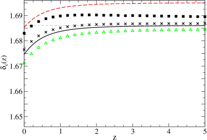
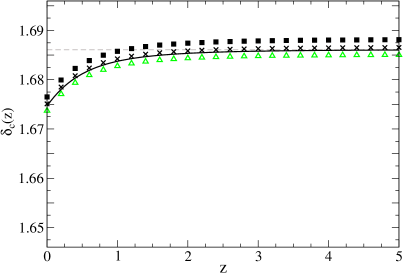
Figure 6: The critical overdensity $\delta_{c}(z)$ as a function of the redshift for the different models considered in the paper. The CDM and $\Lambda$CDM determinations of $\delta_{c}(z)$ (with $\Omega_{m}^{0}=0.284$) are represented by the dashed gray and solid black lines respectively. For the $\Lambda_{t}G_{t}$CDM model, we study the case where we allow for perturbations in $\rho_{\Lambda}$ and $G$ (left panel), with $\Omega_{m}^{0}=0.283$ and three different values of $\nu$ ($\nu=-0.004$, black squares; $\nu=-0.001$, black crosses; $\nu=0.002$, green triangles) – cf. Table 1 of Sect. 7.2. Furthermore, for this model we also consider the situation where these perturbations are neglected (right panel). Finally, the dashed red line in the left panel corresponds to the best fit value for the $\Lambda_{t}$CDM model (i.e. $\Omega_{m}^{0}=0.284$, $\nu=-0.0017$). The precise values $\delta_{c}(0)$ for the two RG models with different inputs are also collected in Table 1 of Sect. 7.2

For comparison, we have also computed $\delta_{c}(z)$ by neglecting the perturbations in $G(a)$ and $\rho_{\Lambda}(a)$ ($\delta G=\delta_{\Lambda}=0$). This would correspond to the canonical or simplest approach (i) mentioned in subsection 7.1. Although the variable $G(a)$ and $\rho_{\Lambda}(a)$ affect now the dynamics only at the background level, they do influence non-trivially the evolution of the matter perturbations through the modified Hubble function. Indeed, in this approach, we have to solve equations (101) and (102) for $\delta G=0$, with $H(a)$ given by (27) – where both $G$ and $\rho_{\Lambda}$ are variable. Alternatively, we may use formally the same approach as in [38] (in which $\delta G=0$ and $G=G_{0}$) if we employ our equations (57)-(58) and the non-trivial effective EoS given by (60). The corresponding solution for $\delta_{c}(z)$ is displayed in the right panel of Fig. 6. We can see that there are some differences with respect to the results obtained in the left panel for non-vanishing perturbations of $\rho_{\Lambda}$ and $G$, but the numerical deviations are not dramatic (at the few per mil level).

The $\Lambda_{t}$CDM model:

As before, we want to derive the second-order differential equation governing the non-linear evolution of the matter perturbations. In this case, however, the continuity equation involves exchange of energy between matter and vacuum:

$$\frac{\partial\rho_{m}}{\partial t}+\nabla_{\vec{r}}\cdot(\rho_{m}\vec{v})=-\dot{\rho}_{\Lambda}\;.$$ (103)

The Euler and Poisson equations (89) and (90) remain unchanged, although we should remark that the Newton’s coupling $G_{N}=G_{0}$ is now strictly constant. As before, we introduce comoving coordinates and define the perturbations as in (91) – (93), but now (consistently with the approach we took in the paper) we will neglect the potential perturbations in the running cosmological constant density $\rho_{\Lambda}$ [so in (91) we set $i=m$]. Inserting Eqs. (91)–(93) into Eqs. (103), (89) and (90) we have:

$$\dot{\delta}_{m}+(1+\delta_{m})\vec{\nabla}\cdot\vec{u} = -Q(t)\delta_{m}\;,$$ (104)

$$\frac{\partial\vec{u}}{\partial t}+2H\vec{u}+(\vec{u}\cdot\vec{\nabla})\vec{u}+\frac{1}{a^{2}}\vec{\nabla}\phi = 0\;,$$ (105)

$$\nabla^{2}\phi-4\pi G_{0}a^{2}\bar{\rho}_{m}\delta_{m} = 0\;,$$ (106)

where $Q(t)$ was defined in Sect. 4, see equation (56). By taking the divergence of the Euler equation (105) [using once more the identity (98)], the time derivative of the continuity equation (104) and combining all three equations, we arrive at the fully non-linear evolution equation:

$$\ddot{\delta}_{m}+\left(2H+Q\right)\dot{\delta}_{m}-\frac{4\dot{\delta}_{m}^{2}+5Q\delta_{m}\dot{\delta}_{m}+Q^{2}\delta_{m}^{2}}{3(1+\delta_{m})}+\left[2HQ+\dot{Q}-4\pi G_{0}\bar{\rho}_{m}(1+\delta_{m})\right]\delta_{m}=0\,,$$ (107)

where we also used the background continuity equation (10). As expected, in the linear regime (107) reduces to equation (55) of Sect. 4:

$$\ddot{\delta}_{m}+(2H+Q)\dot{\delta}_{m}-\left[4\pi\,G_{0}{\bar{\rho}_{m}}-2HQ-\dot{Q}\right]\delta_{m}=0\,.$$ (108)

It is convenient to change the independent variable from $t$ to $a$ and perform the numerical integration of (107) and (108) following the two-step procedure 1) and 2) described in detail above. In particular, equation (108) can be rewritten in the scale factor variable as

$$\delta_{m}^{\prime\prime}+\left(\frac{3}{a}+\frac{H^{\prime}}{H}+\frac{Q}{aH}\right)\delta_{m}^{\prime} - \left[\frac{3}{2}\tilde{\Omega}_{m}(a)-\frac{2Q}{H}-\frac{a}{H}Q^{\prime}\right]\frac{\delta_{m}}{a^{2}}=0\,,$$ (109)

where again $f^{\prime}=\partial_{a}f$ for any quantity $f$ in this equation. For the particular case of time independent vacuum energy ($\dot{\rho}_{\Lambda}=0$) we have $Q=Q^{\prime}=0$, and then upon using $\tilde{\Omega}_{m}(a)=\Omega_{m}^{0}/\left(a^{3}\,E^{2}(a)\right)$ we see that (109) boils down to equation (19) of Ref. [38], as it should. The solution of (109), as a part of the aforementioned two-step procedure, provides $\delta_{c}$ as a function of the scale factor or as a function of the redshift $z=(1-a)/a$, as shown in the left panel of Fig. 6 (see the dashed red line in that figure). For the numerical analysis we used the inputs $\Omega_{m}^{0}=0.284$ and $\nu=-0.0017$, as indicated in Table 1. The corresponding result for $\delta_{c}\equiv\delta_{c}(z=0)$ can be directly read off Fig. 6, and is quoted in that table.

From the range of $\delta_{c}$ values obtained in Table 1 for the two models, we see that they vary from $1.671$ to $1.685$, and hence correspond to variations of $-2.4$ per mil and $+5.9$ per mil, respectively, compared to the $\Lambda$CDM model value ($\delta_{c}(0)=1.675$).

References

- [1] M. Tegmark, et al., Astrophys. J., 606 (2004) 702; D.N. Spergel, et al., Astrophys. J. Suplem., 170 (2007) 377; T.M. Davis et al., Astrophys. J., 666 (2007) 716; M. Kowalski, et al., Astrophys. J., 686 (2008) 749.
- [2] M. Hicken et al., Astroplys. J., 700 (2009) 1097.
- [3] E. Komatsu, et al., Astrophys. J. Suplem., 180 (2009) 330; E. Komatsu, et al., Astrophys. J. Suplem., 192 (2011) 18.
- [4] R. Knop et al., Astrophys. J. 598 (2003) 102; A. Riess et al. Astrophys. J. 607 (2004) 665.
- [5] S. Weinberg, Rev. Mod. Phys. 61 (1989) 1.
- [6] P.J.E. Peebles and B. Ratra, Rev. Mod. Phys. 75 (2003) 559; T. Padmanabhan, Phys. Rep. 380 (2003) 235; V. Sahni, A. Starobinsky, Int. J. of Mod. Phys. A9 (2000) 373; S.M. Carroll, Living Rev. Rel. 4 (2001) 1; E.J. Copeland, M. Sami, S. Tsujikawa, Int. J. of Mod. Phys. D15 (2006) 1753.
- [7] Y. B. Zeldovich, Cosmological constant and elementary particles, Sov. Phys. JETP Lett 6 (1967) 3167; Soviet Physics Uspekhi 11 (1968) 381.
- [8] P.J. Steinhardt, in: Critical Problems in Physics, edited by V.L. Fitch, D.R. Marlow and M.A.E. Dementi (Princeton Univ. Pr., Princeton, 1997); P.J. Steinhardt, Phil. Trans. Roy. Soc. Lond. A361 (2003) 2497.
- [9] F. Bauer, J. Solà, H. Štefančić, Dynamically avoiding fine-tuning the cosmological constant: the “Relaxed Universe”, JCAP 12 (2010) 029, arXiv:1006.3944.
- [10] F. Bauer, J. Solà, H. Štefančić, Phys. Lett. B688 (2010) 269, arXiv:0912.0677.
- [11] F. Bauer, J. Solà, H. Štefančić, Phys. Lett. B 678 (2009) 427, arXiv:0902.2215; F. Bauer, Class. Quant. Grav. 27 (2010) 055001, arXiv:0909.2237; J.Phys. Conf. Ser. 259 (2010) 012083, arXiv:1010.1106; H. Štefančić, Phys. Lett. B670 (2009) 246.
- [12] J. Solà, H. Štefančić, Mod. Phys. Lett. A21 (2006) 479, astro-ph/0507110; Phys. Lett. B624 (2005) 147, astro-ph/0505133; J. Phys. A39 (2006) 6753, gr-qc/0601012.
- [13] J. Grande, J. Solà and H. Štefančić, JCAP 08 (2006) 011, gr-qc/0604057; Phys. Lett. B645 (2007) 236, gr-qc/0609083; J. Phys. A: Math. Theor. 40 (2007) 6787, gr-qc/0701090; J. Phys. A: Math. Theor. 40 (2007) 6935, astro-ph/0701201; J. Grande, A. Pelinson, J. Solà, Phys. Rev. D79 (2009) 043006, arXiv:0809.3462; J. Grande, R. Opher, A. Pelinson, and J. Solà, JCAP 0712 (2007) 007, arXiv:0709.2130; J. Grande, A. Pelinson, and J. Solà, proc. of the 7th Int. Heidelberg Conference, Dark 2009, edited by H. V. Klapdor-Kleingrothaus and I. V. Krivosheina (World Scientific, Singapore, 2009) p. 380, arXiv:0904.3293.
- [14] J. Solà, Cosmologies with a time dependent vacuum, J. Phys. Conf. Ser. 283 (2011) 012033, arXiv:1102.1815.
- [15] N.C. Tsamis, R.P. Woodard, Phys. Rev. D81 (2010) 103509, arXiv:1001.4929; Phys. Rev. D80 (2009) 083512, arXiv:0904.2368.
- [16] M. Maggiore, Phys. Rev. D83 (2011) 063514, arXiv:1004.1782; N. Bilic, Phys. Rev. D83 (2011) 105003, arXiv:1104.1349; G. Mangano, Phys. Rev. D82 (2010) 043519, arXiv:1005.2758.
- [17] F.R. Klinkhamer, G.E. Volovik, Phys. Rev. D78 (2008) 063528, arXiv:0806.2805; arXiv:1102.3152; D.A. Demir, Found. Phys. 39 (2009) 1407; V. Branchina, D. Zappala, Gen. Rel. Grav 42 (2010) 141; Mod. Phys. Lett. A25 (2010) 2305; J. Beltran Jiménez, A. L. Maroto, JCAP 0903 (2009) 016; P. Batra, K. Hinterbichler, L. Hui, D.N. Kabat, Phys. Rev. D78 (2008) 043507; S. M. Barr, S. P. Ng and R. J. Scherrer, Phys. Rev. D73 (2006) 063530; Y. Du, H. Zhang, X.-Z. Li, arXiv:1008.4421; M. M. Verma, Astrophys. Space Sci. 330 (2010) 101; B. Feng, X.L. Wang and X.M. Zhang, Phys. Lett. B607 (2005) 35.
- [18] S. Ray, M.Yu.Khlopov, P. P. Ghosh and U. Mukhopadhyay, Int. J. Theor. Phys. 50 (2011) 939, arXiv:0711.0686; M. M. Verma, Astrophys. Space Sci. 330 (2010) 101; G. Leon, Y. Leyva, E. N. Saridakis, O. Martin, R. Cardenas, arXiv:0912.0542; J. Lu, E. N. Saridakis, M.R. Setare, L. Xu, JCAP 03 (2010) 031, arXiv:0912.0923; M. Jamil, E. N. Saridakis, M.R. Setare Phys. Lett. B679 (2009) 172, arXiv:0906.2847.
- [19] A.D. Dolgov, in: The very Early Universe, Ed. G. Gibbons, S.W. Hawking, S.T. Tiklos (Cambridge U., 1982); L.F. Abbott, Phys. Lett. B150 (1985) 427; L.H. Ford, Phys. Rev. D35 (1987) 2339; R.D. Peccei, J. Solà and C. Wetterich, Phys. Lett. B195 (1987) 183; S. M. Barr, Phys. Rev. D36 (1987) 1691; S. M. Barr and D. Hochberg, Phys. Lett. B211 (1988) 49; J. Solà, Phys. Lett. B228 (1989) 317; Int. J. of Mod. Phys. A5 (1990) 4225.
- [20] C. Wetterich, Nucl. Phys. B302 (1988) 668; P.J.E. Peebles and B. Ratra, Astrophys. J. 325 (1988) L17; B. Ratra and P.J.E. Peebles, Phys. Rev. D37 (1988) 3406; P.G. Ferreira and M. Joyce, Phys. Rev. D58 (1998) 023503; R.R. Caldwell, R. Dave and P.J. Steinhardt, Phys. Rev. Lett. 80 (1998) 1582; P.J. Steinhardt, L.M. Wang and I. Zlatev, Phys. Rev. D59 (1999) 123504; V. Sahni and L.M. Wang, Phys. Rev. D62 (2000) 103517.
- [21] O. Bertolami, Nuovo Cimento, 93B, 36, (1986); M. Ozer M. and O. Taha, Nucl. Phys., B287, 776, (1987); O. K. Freese K., et al., Nucl. Phys., 287, 797, (1987); J. C. Carvalho, J. A. S. Lima and I. Waga, Phys. Rev. D46, 2404, (1992); W. Chen and Y-S. Wu, Phys. Rev. D 41, 695 (1990); J. A. S. Lima and J. M. F. Maia, Phys. Rev D 49, 5597 (1994); J. A. S. Lima, Phys. Rev. D 54, 2571 (1996), [gr-qc/9605055]; A. I. Arbab and A. M. M. Abdel-Rahman, Phys. Rev. D 50, 7725 (1994).
- [22] J. M. Overduin and F. I. Cooperstock, Phys. Rev. D., 58, 043506, (1998), and references therein.
- [23] J. Solà, J. of Phys. A41 (2008) 164066, arXiv:0710.4151.
- [24] I. L. Shapiro, J. Solà, Phys. Lett. B682 (2009) 105, arXiv:0910.4925; see also the detailed review arXiv:0808.0315 on the quantum field theory of the CC term.
- [25] S. Basilakos, Astronomy & Astrophysics, 508 (2009) 575.
- [26] B.F.L. Ward, Mod. Phys. Lett. A25 (2010) 607, arXiv:0908.1764, and arXiv:0910.0490; Int. J. Mod. Phys. D17 (2008) 627, hep-ph/0610232; and Mod. Phys. Lett. A23 (2008) 3299, arXiv:0808.3124; B. Koch, I. Ramirez, Class. Quant. Grav. 28 (2011) 055008,arXiv:1010.2799.
- [27] I.L. Shapiro, J. Solà, JHEP 02 (2002) 006, hep-th/0012227; Phys. Lett. 475B (2000) 236, hep-ph/9910462.
- [28] I.L. Shapiro, J. Solà, C. España-Bonet, P. Ruiz-Lapuente, Phys. Lett. 574B (2003) 149, astro-ph/0303306; JCAP 0402 (2004) 006, hep-ph/0311171; I.L. Shapiro, J. Solà, Nucl. Phys. Proc. Suppl. 127 (2004) 71, hep-ph/0305279; JHEP proc. AHEP2003/013, astro-ph/0401015.
- [29] A. Babic, B. Guberina, R. Horvat, H. Štefančić, Phys. Rev. D65 (2002) 085002; B. Guberina, R. Horvat, H. Štefančić, Phys. Rev. D67 (2003) 083001; I.L. Shapiro, J. Solà, H. Štefančić, JCAP 0501 (2005) 012, hep-ph/0410095; F. Bauer, Class. Quant. Grav. 22 (2005) 3533; F. Bauer, Ph.d. Thesis, hep-th/0610178; gr-qc/0512007.
- [30] L.E. Parker and D.J. Toms, Quantum Field Theory in Curved Spacetime: quantized fields and gravity (Cambridge U. Press, 2009).
- [31] S. Basilakos, M. Plionis and J. Solà, Phys. Rev. D80 (2009) 083511, arXiv:0907.4555.
- [32] O. Lahav, P. B. Lilje, J. R. Primack, &, M. J. Rees, Mon. Not. Roy. Astron. Soc., 251 (1991) 128; L. Wang, & J. P. Steinhardt, Astrophys. J. 508 (1998) 483; I. T. Iliev, &, P. R. Shapiro, Mon. Not. Roy. Astron. Soc., 325 (2001) 468; E. L. Lokas, Acta Physica Polonica B32 (2001) 3643; R. A. Battye and J. Weller, Phys. Rev. D68 (2003) 083506; R. Mainini, A. W. Maccio, S. A. Bonometto, &, A. Klypin, Astrophys. J., 599 (2003) 24;
- [33] L.R. Abramo, R.C. Batista, L. Liberato, R. Rosenfeld, JCAP 0711, 012 (2007), arXiv:0707.2882; Phys.Rev. D79 (2009) 023516, arXiv:0806.3461.
- [34] N. N., Weinberg, M. Kamionkowski, Astrophys. J., 341 (2003) 251, astro-ph/0210134.
- [35] D. F. Mota &, C. van de Bruck C., Astronomy & Astrophysics, 421, 71, (2004).
- [36] N. J. Nunes, &, D. F. Mota, Mon. Not. Roy. Astron. Soc., 368, 751, (2006); M.Manera and D. F. Mota, Mon. Not. Roy. Astron. Soc. 371, 1373 (2006); C. Horellou & J. Berge, Mon. Not. Roy. Astron. Soc., 360, 1393, (2005); Ding-fang Zeng, &, Yi-hong Gao, 2005, (astro-ph/0505164); I. Maor, &, O. Lahav, Journal of Cosmology and Astroparticle Physics, 7, 3, (2005); W. J. Percival, Astronomy & Astrophysics, 443, 819, (2005); P. Wang, Astrophys. J., 640, 18, (2006); M. Bartelmann, M. Doran and C. Wetterich, Astron. & Astrophys., 454 (2006) 27.
- [37] S. Basilakos, &, N. Voglis, Mon. Not. Roy. Astron. Soc., 374, 269, (2007); S. Basilakos, J. C. Sanchez, L. Perivolaropoulos, Phys. Rev. D., 80 (2009) 3530.
- [38] F. Pace, J.-C Waizmann and M. Bartelmann, Mon. Not. Roy. Astron. Soc. 406 (2010) 1865, arXiv:1005.0233.
- [39] F. Schmidt, W. Hu, and M. Lima, Phys. Rev. D., 81 (2010) 3005, arXiv:0911.5178.
- [40] S. Basilakos, M. Plionis and J.A.S. Lima, Phys. Rev. D 82 (2010) 3517, arXiv:1006.3418.
- [41] S. Basilakos, M. Plionis and J. Solà, Phys. Rev. D82 (2010) 083512, arXiv:1005.5592.
- [42] J. Grande and J. Solà, in preparation; J. Grande, PhD Thesis, Univ. de Barcelona (2010).
- [43] B.L. Nelson and P. Panangaden, Phys. Rev. D25 (1982) 1019; D.J. Toms, Phys. Lett. B126 (1983) 37; L. Parker, D.J. Toms, Phys. Rev. D29 (1984) 1584; Phys. Rev. D32 (1985) 1409.
- [44] A. Bonanno, M. Reuter, Phys. Rev. D 62, 043008, (2000), hep-th/0002196; Phys. Rev. D65 (2002) 043508; E. Bentivegna, A. Bonanno, M. Reuter, JCAP 01 (2004) 001.
- [45] J. Grande, J. Solà, J. C. Fabris, I. L. Shapiro, Class. Quant. Grav. 27 (2010) 105004, arXiv:1001.0259.
- [46] I.L. Shapiro, J. Solà, H. Štefančić, JCAP 0501 (2005) 012, hep-ph/0410095.
- [47] D. C. Rodrigues, P. S. Letelier, I. L. Shapiro, JCAP 1004 (2010) 020, arXiv:0911.4967; S. Domazet, H. Štefančić, arXiv:1010.3585; Yun-He Li, Xin Zhang, arXiv:1103.3185.
- [48] M.T. Murphy, J.K. Webb, V.V. Flaumbaum, Mon. Not. Roy. Astron. Soc. 345 (2003) 609.
- [49] P. Jordan, Nature 164 (1949) 637; C. Brans, R.H. Dicke, Phys. Rev. D124 (1961) 925.
- [50] H. A. Borges, S. Carneiro, J. C. Fabris, Phys. Rev. D78 123522, (2008); M.L. Tong, H. Noh, arXiv:1102.3254.
- [51] P. Wang, X.-H. Meng, Class. Quant. Grav. 22 (2005) 283, astro-ph/0408495.
- [52] J. S. Alcaniz and J. A. S. Lima, Phys. Rev. D 72, 063516 (2005), astro-ph/0507372.
- [53] P.J.E. Peebles, “Principles of Physical Cosmology”, Princeton University Press, Princeton New Jersey (1993).
- [54] J. Fabris, I.L. Shapiro, J. Solà, JCAP 02 (2007) 016, gr-qc/0609017; A.M. Velasquez-Toribio, arXiv:0907.3518.
- [55] D. J. Eisenstein et al., Astrophys. J., 633, 560, (2005); N. Padmanabhan, et al., Mon. Not. Roy. Astron. Soc., 378 (2007) 852.
- [56] W. Percival et al., Mon. Not. Roy. Astron. Soc., 401 (2010) 2148.
- [57] E. A. Kazin, Astrophys. J., 710 (2010) 1444.
- [58] D. J. Eisenstein, and W. Hu, Astrophys. J., 496 (1998) 605.
- [59] J. R. Bond, G. Efstathiou and M. Tegmark, Mon. Not. Roy. Astron. Soc. 291 (1997) L33.
- [60] S. Nesseris and L. Perivolaropoulos, JCAP 0701 (2007) 018.
- [61] O. Elgaroy & T. Multamaki, JCAP 9, 2 (2007); P.S. Corasaniti & A. Melchiorri Phys.Rev.D, 77 (2008) 103507.
- [62] W.H. Press and P. Schechter, Astrophys. J. 187 (1974) 425.
- [63] V. Eke, S. Cole &, C. S. Frenk, Mon. Not. Roy. Astron. Soc., 282 (1996) 263.
- [64] J. M. Bardeen, J. R. Bond, N. Kaiser, and, A. S. Szalay, Astrophys. J., 304 (1986) 15.
- [65] N. Sugiyama, Astrophys. J. Suplem., 100 (1995) 281.
- [66] A. Jenkins, et al., Mon. Not. Roy. Astron. Soc., 321 (2001) 372.
- [67] L. Marassi and J. A. S. Lima, Int. J. Mod. Phys. D 13, 1345 (2004) and D 16 (2007) 445.
- [68] D. Reed, R. Bower, C. Frenk, A. Jenkins, and T. Theuns, MNRAS 374 (2007) 2.
- [69] E. Rozo, et al., Astrophys. J., 708 (2010) 645.
- [70] L. Fu, et al., Astron. Astrophys. 479 (2008) 9.
- [71] A.G. Sánchez, M. Crocce, A. Cabré, C. M. Baugh and E. Gaztañaga, Mon. Not. Roy. Astron. Soc., 400 (2009) 1643.
- [72] L.D. Ferramacho, A. Blanchard and Y. Zolnierowski, Astron. Astrophys. 499 (2009) 21, arXiv:0807.4608.
- [73] R. W. Pike, and, M. J. Hudson, Astroplys. J., 635, 11 (2005); A. Cabré, and, E. Gaztanaga, Mon. Not. Roy. Astron. Soc. 393 (2009) 1183.
- [74] H. Feldman, R. Juszkiewicz, P. Ferreira, M. Davis, E. Gaztañaga, J. Fry, A. Jaffe, S. Chambers, L. da Costa, M. Bernardi, R. Giovanelli, M. Haynes, G. Wegner, Astrophys. J., 596 (2003) L131.
- [75] C. Fedeli, L. Moscardini, and S. Matarrese, Mon. Not. Roy. Astron. Soc., 397 (2009) 1125.
- [76] J.C. Raymond and B.W. Smith, Astroplys. J. Suppl. 35 (1977) 419.