A Bayesian study of the primordial power spectrum from a novel closed universe model

Abstract

We constrain the shape of the primordial power spectrum using recent measurements of the cosmic microwave background (CMB) from the Wilkinson Microwave Anisotropy Probe (WMAP) 7-year data and other high-resolution CMB experiments. We also include observations of the matter power spectrum from the luminous red galaxy (LRG) subset DR7 of the Sloan Digital Sky Survey (SDSS). We consider two different models of the primordial power spectrum. The first is the standard nearly scale-invariant spectrum in the form of a generalised power-law parameterised in terms of the spectral amplitude $A_{\rm s}$, the spectral index $n_{\rm s}$ and (possibly) the running parameter $n_{\rm run}$. The second spectrum is derived from the Lasenby and Doran (LD) model. The LD model is based on the restriction of the total conformal time available in a closed Universe and the predicted primordial power spectrum depends upon just two parameters. An important feature of the LD spectrum is that it naturally incorporates an exponential fall-off on large scales, which might provide a possible explanation for the lower-than-expected power observed at low multipoles in the CMB. In addition to parameter estimation, we compare both models using Bayesian model selection. We find there is a significant preference for the LD model over a simple power-law spectrum for a CMB-only dataset, and over models with an equal number of parameters for all the datasets considered.

1 Introduction

Cosmological inflation not only explains the homogeneity of the universe on large scales, but also provides a theory for explaining the observed level of anisotropy (Guth 1981; Albrecht & Steinhardt 1982; Mukhanov & Chibisov 1982). Inflationary models generically predict Gaussian, adiabatic and nearly scale-invariant primordial fluctuations. To determine the shape of the primordial power spectrum from cosmological observations, it is usual to assume a parameterised form for it. The simplest assumption is that the initial spectrum has the form of a simple power-law, parameterised in terms of the spectral amplitude $A_{\rm s}$ and the spectral index $n_{\rm s}$. Recent analyses have shown, however, that the spectral index may deviate from a constant value (close to unity) and so consideration of models that provide some running of the index (defined by $n_{\rm run}\equiv dn_{\rm s}/d\ln k$) is warranted. Furthermore, models that predict a decrement in CMB power at low multipoles seem to be preferred by observations (Efstathiou 2003; Contaldi et al. 2003), so that, an extra variable to account for a cut-off scale might be considered. It would be feasible to continue adding parameters in this fashion until some arbitrary accuracy of model fit is achieved, but this procedure would fail to account for Occam’s razor: a simpler model should be preferred, unless the data require a more sophisticated one. Using the Bayesian evidence to select between models is one way to include this consideration.

There have been several recent studies regarding the shape of the primordial spectrum, some based on physical models, some using observational data to constrain an a priori parameterisation, and others attempting a direct reconstruction from data (Barriga et al. 2001; Bridle et al. 2003; Hannestad 2004; Bridges et al. 2006, 2007, 2009; Verde & Peiris 2008; Peiris & Verde 2010; Hlozek et al. 2011; Guo et al. 2011). A primary goal of this work is to fit the predicted form of the primordial spectrum from a physically motivated model described by Lasenby & Doran (2005) (henceforth LD). We translate observational data into constraints on the generalised power-law and LD forms for the primordial power spectrum (and the standard cosmological parameters), and decide which model provides the best fit to observational data using the Bayesian evidence.

The paper is organised as follows: in Section 2 we present the two different models for the power spectrum and in Section 3 we describe basic parameter estimation and model selection. We list the datasets and the cosmological parameters considered in Section 4 and present the resulting parameter constraints in Section 5. We compute Bayesian evidences in Section 6 to decide which model provides the best description for current observational data and we validate our analysis by applying it to a CMB simulated data. Our conclusions are presented in Section 7.

2 Primordial power spectrum

The correlation function $\xi$ of density fluctuations $\delta\equiv\delta\rho/\rho$ at two separated points $\mn@boldsymbol{x}$ and $\mn@boldsymbol{x}+\mn@boldsymbol{r}$ is defined as

$$\xi(r)\equiv\langle\delta(\mn@boldsymbol{x})\delta(\mn@boldsymbol{x}+\mn@boldsymbol{r})\rangle.$$ (1)

Because the assumption of homogeneity and isotropy, $\xi$ is a function only of $r\equiv|\mn@boldsymbol{r}|$. The power spectrum $\mathcal{P}(k)$ describes the amplitude of fluctuations on different length scales and it is related with the inverse Fourier transform of the correlation function $\xi$ by:

$$\mathcal{P}(k)\equiv\langle|\delta_{k}|^{2}\rangle.$$ (2)

During the inflationary period, fluctuations in the inflaton field $\delta\phi_{k}$ result in curvature perturbations $\mathcal{R}(k)$ given by

$$\mathcal{R}(k)=-\left[\frac{H}{\dot{\phi}}\delta\phi_{k}\right]_{k=RH},$$ (3)

where the quantities are evaluated at the horizon exit epoch $k=RH$. Here $R$ is the scale factor of the universe and $H\equiv\dot{R}/{R}$ is the Hubble parameter. In this paper, we follow a slow-roll approximation (e.g. Liddle & Lyth 1999). Hence the power spectrum of the inflaton fluctuations is constant in time and equal to

$$\mathcal{P}_{\delta\phi}(k)=\left(\frac{H}{2\pi}\right)^{2}_{k=RH}.$$ (4)

Thus, the primordial curvature spectrum $\mathcal{P_{R}}(k)$ computed from (2) - (4) is

$$\mathcal{P_{R}}(k)=\left[\left(\frac{H}{\dot{\phi}}\right)^{2}\left(\frac{H}{2\pi}\right)^{2}\right]_{k=RH}.$$ (5)

2.1 Power-law parameterisations

Cosmological slow-roll inflation predicts the spectrum of curvature perturbations to be close to scale-invariant. Based on this, the spectrum is commonly assumed to have the form

$$\mathcal{P_{R}}(k)=A_{\rm s}\left(\frac{k}{k_{0}}\right)^{n_{\rm s}-1},$$ (6)

where the spectral index $n_{\rm s}$ is expected to be close to unity; $k_{0}$ is the pivot scale (set to $k_{0}=0.05$ $\rm{Mpc}^{-1}$ throughout). A spectrum where the typical amplitude of perturbations is identical on all length scales is known as Harrison-Zel’dovich spectrum ($n_{\rm s}=1$).This particular parameterisation involves only one free parameter, the spectral amplitude $\mathcal{P}(k)=A_{\rm s}$.

A further extension is possible by allowing the spectral index to vary as a function of scale, such that $n_{\rm s}(k)$. This can be achieved by including a second order term in the expansion of the power spectrum

$$\mathcal{P_{R}}(k)=A_{\rm s}\left(\frac{k}{k_{0}}\right)^{n_{\rm s}-1+(1/2)\ln(k/k_{0})(dn/d\ln k)},$$ (7)

where $dn/d\ln k$ is termed the running parameter $n_{\rm run}$ and we would expect $n_{\rm run}\approx 0$ for standard inflationary models.

In what follows we will consider three Power-Law parameterisations. In the first model (PL 1), we will assume a simple power-law spectrum (without running) and restrict the universe to be spatially flat. In PL model 2, we allow the spatial curvature of the universe to be a free parameter. In PL model 3, we allow for a running spectrum, but again restrict the universe to be spatially-flat. In this way, power-law models 2 and 3 have the same number of parameters.

2.2 The LD model

Assuming the cosmological constant is the origin of dark energy, Lasenby & Doran (2005) provided a construction for embedding closed-universe models in a de Sitter background. As a consequence of this novel approach, a boundary condition on the total available conformal time emerges. Defining the total conformal time $\eta$ as

$$\eta\equiv\int^{\infty}_{0}\frac{dt}{R(t)},$$ (8)

the LD model requires $\eta=\pi/2$. For more details about the choice of the boundary condition, including how it can be reinterpreted as an eigenvalue condition on the solution of a differential equation, see Lasenby (2003); Lasenby & Doran (2004, 2005). In order to understand some consequences of the new boundary condition we split the history of the Universe in two main contributions to the total conformal time: matter (radiation and dust) and inflationary eras. Hence, we want to compute the conformal time $\eta_{\rm M}$ elapsed during the matter era and add it to that elapsed in the inflationary era $\eta_{\rm I}$, such that the boundary condition is satisfied:

$$\eta_{\rm I}+\eta_{\rm M}=\frac{\pi}{2}.$$ (9)

It is found that this constraint leads to a ‘see-saw’ mechanism linking the parameters describing the current state of the universe with the initial conditions (Lasenby & Doran 2004).

2.2.1 Matter era

The general description of the large scale Universe is based on the Robertson-Walker space-time with dynamics governed by the Einstein equations. The resulting Friedmann equations can be written as (with $c=1$)

$$\frac{\dot{R}^{2}+k}{R^{2}}-\frac{\Lambda}{3} = \frac{8\pi G}{3}\,\rho,$$ (10)

$$2\frac{\ddot{R}}{R}+\frac{\dot{R}^{2}+k}{R^{2}}-\Lambda = -8\pi GP.$$

Here $k=0$, $\pm 1$ defines the geometry of the universe, $\Lambda$ is the cosmological constant, and the relationship between density $\rho$ and pressure $P$ is encoded in the equation of state $P=\gamma\rho$. The behaviour of the homogeneous universe is governed by the parameters representing its matter-energy content, namely

$$\Omega_{M}=\frac{8\pi G\rho}{3H^{2}},\qquad\qquad\Omega_{\Lambda}=\frac{\Lambda}{3H^{2}},$$ (11)

and its expansion history defined by the Hubble parameter $H$. Moreover, if we assume the matter density is made up of decoupled dust and radiation, the equations governing $\Omega_{M}$ and $\Omega_{\Lambda}$ can be solved exactly and its solution is controlled by two arbitrary constants $\alpha$ and $\beta$ given by

$$\alpha = \frac{\Omega_{m_{o}}^{2}\Omega_{\Lambda_{o}}}{(\Omega_{m_{o}}+\Omega_{r_{o}}+\Omega_{\Lambda_{o}}-1)^{3}},$$ (12)

$$\alpha\beta = \frac{\Omega_{r_{o}}\Omega_{\Lambda_{o}}}{(\Omega_{m_{o}}+\Omega_{r_{o}}+\Omega_{\Lambda_{o}}-1)^{2}},$$

where subscript ‘$o$’ denotes quantities evaluated at present time. The total conformal time for this type of universe can be written in terms of the dimensionless parameters $\alpha$ and $\beta$ as (see Lasenby & Doran 2005)

$$\eta_{M}=\int^{\infty}_{0}\frac{dx}{(\beta x^{4}+x^{3}-x^{2}+\alpha)^{1/2}}.$$ (13)

2.2.2 Inflationary era

The computation of the conformal time in the inflationary epoch is a more elaborate process. Let us consider a basic inflationary model where the particle responsible for this process is simply a real, time-dependent, homogeneous, free, massive scalar field $\phi$, described by the equations

$$\dot{H}+H^{2}-\frac{\Lambda}{3}+\frac{4\pi G}{3}(2\dot{\phi}^{2}-m^{2}\phi^{2}) = 0,$$

$$\ddot{\phi}+3H\dot{\phi}+m^{2}\phi = 0.$$ (14)

For closed universe models, the scale factor is given explicitly by

$$\frac{1}{R^{2}}=\frac{4\pi G}{3}(\dot{\phi}^{2}+m^{2}\phi^{2})-H^{2}+\frac{\Lambda}{3}.$$ (15)

In order to compute the conformal time $\eta_{I}$, it is necessary to seek out suitable conditions before the onset of inflation and then solve the dynamics for the scalar field encoded in equations (14). To do this, Lasenby & Doran (2005) developed formal series expansions out of the initial singularity, $t=0$, in terms of dimensionless variables $u=t/t_{\rm p}$ and $\mu=m/m_{\rm p}$, where the subscript ‘p’ denotes a Planck units variable. The series are given by

$$\phi(u) = \frac{1}{l_{\rm p}}\sum_{n=0}^{\infty}\phi_{n}(u)\ln^{n}(u),$$

$$H(u) = \frac{1}{t_{\rm p}}\sum_{n=0}^{\infty}H_{n}(u)\ln^{n}(u),$$ (16)

with

$$\phi_{0} = b_{0}+b_{4}u^{4/3}-\frac{118\sqrt{3\pi}b_{4}^{2}}{99}u^{8/3}-\frac{u^{2}}{1296\pi}(11\sqrt{3\pi}\mu^{2}$$

$$-54\sqrt{3\pi}\Lambda-216\sqrt{3}\pi^{3/2}\mu^{2}b_{0}^{2}+36\pi\mu^{2}b_{0}),$$

$$\phi_{1} = -\sqrt{\frac{1}{12\pi}}-\frac{\mu^{2}}{216\pi}\left(-\sqrt{3\pi}+36\pi b_{0}\right)u^{2},$$

$$H_{0} = \frac{1}{3u}+\frac{32\sqrt{3\pi}}{27}b_{4}u^{1/3}+(\frac{2\mu^{2}}{81}+\frac{\Lambda}{3}+\frac{4\pi}{3}\mu^{2}b_{0}^{2}$$

$$+\frac{4\sqrt{3\pi}}{27}\mu^{2}b_{0})u-\frac{6656\pi b_{4}^{2}}{891}u^{5/3},$$

$$H_{1} = -u\frac{dH_{0}}{du}-uH_{0}^{2}+\frac{u\Lambda}{3}-\frac{8\pi\ u}{3}\left(\frac{d\phi_{0}}{du}\right)^{2}$$ (17)

$$-\frac{16\pi\phi_{1}}{3}\frac{d\phi_{0}}{du}-\frac{8\pi\phi_{1}^{2}}{3u}+\frac{4\pi\mu^{2}u\phi_{0}^{2}}{3}.$$

We observe that two new free parameters $b_{0}$ and $b_{4}$, appear in the series expansions in (2.2.2). Together with the mass of the scalar field $\mu$, they control the magnitude of the field and how long the inflationary period lasts. In order to decide on the priors we shall employ in our subsequent Bayesian analysis, it is worth pointing out some features related with these new parameters.

• The amplitude of the perturbations is determined by the scalar field mass $\mu$. To match the observed level of CMB anisotropies, we shall need to set it to be about

  $$\mu\sim 10^{-6}.$$ (18)

• The number of e-foldings $N$ is primarily determined by $b_{0}$ and may be approximated as

  $$N\approx 2\pi b_{0}^{2}.$$ (19)

  Hence, to obtain realistic models we need $b_{0}$ to be of order $\sim$ a few.

• The conformal time is estimated by

  $$\eta_{I}\approx 0.92\left(\frac{|b_{4}|}{\mu^{4/3}}\right)^{1/2}\left(\frac{1}{b_{0}^{2}}\right).$$ (20)

  Employing the constraint (9), $|b_{4}|\mu^{-4/3}$ should thus be around unity.

• The parameter $b_{4}$ controls the initial curvature, as can be seen from (15):

  $$\frac{R}{l_{\rm p}}\approx\left(\frac{2187}{12544\pi}\right)^{1/4}\frac{u^{1/3}}{\sqrt{-b_{4}}}.$$ (21)

  Therefore $b_{4}$ must be negative. Making use of the rest of the parameters and (20), $|b_{4}|$ should be around $10^{-9}$.

The restriction on the values for the model parameters together with the boundary condition, severely limits the class of models allowed to reproduce current cosmological observations.

Figure 1: Evolution of the conformal time $\eta_{I}$ as a function of $\ln(u)$. We observe that $\eta_{I}$ saturates at a value of around 1.35 by the end of inflation. The parameters used in this model are $b_{0}=2.47$, $b_{4}=-17.7\times 10^{-9}$ and $\mu=1.68\times 10^{-6}$.

Once we have found the initial conditions (2.2.2), it is straightforward to solve numerically the dynamics of the scalar field $\phi$ and the expansion history $H$ to determine the evolution of the universe. As an example, let us consider the best-fit values for the cosmological parameters given by WMAP+BAO+$H_{0}$ (Komatsu et al. 2011), in which case the conformal time elapsed during the matter epoch is $\eta_{M}=0.22$. In order to satisfy the boundary condition we should choose appropriate values $\{b_{0},b_{4},\mu\}$ such that by the end of the inflationary period the achieve conformal time is $\eta_{I}\approx 1.35$, as shown on Fig 1. The expected shape of the primordial power spectrum $\mathcal{P}(k)$ for this model is directly computed from (5).

3 Bayesian analysis

3.1 Parameter Estimation

A Bayesian analysis provides a consistent approach to estimate the set of parameters $\mathbf{\Theta}$ within a model $M$, which best describes the data $\mn@boldsymbol{D}$. The method is based on the assignment of probabilities to all quantities of interest, and then the manipulation of those probabilities given a series of rules, of which Bayes’ theorem plays the principal role, (Bayes 1761). Bayes’ theorem states that

$$P(\mathbf{\Theta}|\mn@boldsymbol{D},M)=\frac{P(\mn@boldsymbol{D}|\mathbf{\Theta},M)\,\,P(\mathbf{\Theta}|M)}{P(\mn@boldsymbol{D}|M)},$$ (22)

where the prior probability $P(\mathbf{\Theta}|M)\equiv\pi$ represents our knowledge of $\mathbf{\Theta}$ before considering the data. This probability is modified through the likelihood $P(\mn@boldsymbol{D}|\mathbf{\Theta},M)\equiv\mathcal{L}$ when the experimental data $\mn@boldsymbol{D}$ are considered. The final objective for Bayesian inference is to obtain the posterior probability $P(\mathbf{\Theta}|\mn@boldsymbol{D},M)$ which represents the state of knowledge once we have taken the new information into account. The normalisation constant is the marginal likelihood or Bayesian evidence $P(\mn@boldsymbol{D}|M)\equiv\mathcal{Z}$. Since this quantity is independent of the parameters $\mathbf{\Theta}$, it is commonly ignored in parameter estimation but takes the central role for model selection (Hobson et al. 2002; Liddle 2004).

3.2 Model selection

A complex model that explains the data slightly better than a simple one should be penalised for the introduction of extra parameters, because the additional parameters bring with them a lack of predictability. Also, if a model is too simple, it might not fit the data equally well, then it can be discarded (e.g. Liddle 2006, 2007; Trotta 2008). Following this line, many attempts have been performed to translate Occam’s razor into a mathematical language for model selection. The prime tool for the model selection we focus on is the Bayesian evidence.

The Bayesian evidence provides a natural mechanism to balance the complexity of cosmological models and then, elegantly, incorporates Occam’s razor. It applies the same type of analysis from parameter estimation but now at the level of models rather than parameters (Trotta 2007). Let us consider several models $M$, each of them with probability $P(M)$. The Bayesian evidence appears again, but now in another form of the Bayes theorem:

$$P(M|\mn@boldsymbol{D})=\frac{P(\mn@boldsymbol{D}|M)P(M)}{P(\mn@boldsymbol{D})}.$$ (23)

The left-hand side denotes the probability of the model given the data, which is exactly what we are looking for model selection.

It was previously mentioned that the Bayesian evidence is simply the normalisation over its posterior expressed by:

$$\mathcal{Z}=\int\mathcal{L}(\textbf{$\Theta$})\pi(\textbf{$\Theta$})d^{N}\textbf{$\Theta$},$$ (24)

where $N$ is the dimensionality of the parameter space. When two models are compared, $M_{0}$ and $M_{1}$, the quantity to bear in mind is the ratio of the posterior probabilities given by

$$\frac{P(M_{0}|\mn@boldsymbol{D})}{P(M_{1}|\mn@boldsymbol{D})}=\,\,\frac{\mathcal{Z}_{0}}{\mathcal{Z}_{1}}\frac{P(M_{0})}{P(M_{1})}=\,\,B_{01}\frac{P(M_{0})}{P(M_{1})},$$ (25)

where $P(M_{0})/P(M_{1})$ is the prior probability ratio for two models, usually set to unity. The evidence ratio, often termed as the Bayes factor $B_{01}$, quantifies how well model $0$ may fit data when it is compared to model 1. Jeffreys (1961) provided a useful guide on which we are able to make qualitative conclusions based on this difference (see Table 1).

Table 1: Jeffreys scale for evaluating the strength of evidence when two models are compared.

$|\ln B_{01}|$	Odds	Probability	Strength of $\mathcal{Z}$
$<$ 1.0	$<$ 3 : 1	$<$ 0.750	Inconclusive
1.0	$\sim$ 3 : 1	0.750	Significant
2.5	$\sim$ 12 : 1	0.923	Strong
$>$ 5.0	$>$ 150 : 1	$>$ 0.993	Decisive

Until recently, numerical methods such as thermodynamic integration (Beltrán et al. 2005; Bridges et al. 2007) required around $10^{7}$ likelihood evaluations to obtain accurate estimates of the Bayesian evidence, making the procedure hardly tractable. The nested sampling algorithm, invented by Skilling (2004), has been successfully implemented for cosmological applications (Mukherjee et al. 2006; Shaw et al. 2007; Feroz et al. 2008) requiring about a hundred times fewer posterior evaluations than thermodynamic integration to achieve the same accuracy in the evidence estimate. A substantially improved and fully-parallelized algorithm called MultiNest (Feroz et al. 2009) increases the sampling efficiency for calculating the evidence and obtaining posterior samples, even from distributions with multiple modes and/or pronounced degeneracies between parameters. In our case, to carry out the exploration of the cosmological parameter space we use a modified version of both the MultiNest (Feroz et al. 2009) and CosmoMC (Lewis & Bridle 2002) packages.

4 Datasets

Measurements of the CMB anisotropies and large-scale structure play an important role in both fitting parameters and comparison of models in cosmology. To constrain the space-parameter in each model, we first use the latest 7-year data release from WMAP (henceforth WMAP7; Larson et al. 2011), which includes a good measurement up to the third acoustic peak in the temperature CMB spectrum. This comprises our dataset 1.

WMAP7 data by itself cannot, however, place strong constraints on all the parameters because of the existence of parameter degeneracies, such as the $\tau-A$ degeneracy and the well-known geometrical degeneracy, involving $\Omega_{\rm m}$, $\Omega_{\Lambda}$ and $\Omega_{k}$. Nevertheless, when WMAP7 is combined with other cosmological observations, they together increase the constraining power and considerably weaken the degeneracies. In addition to WMAP7, we therefore include recent results from CMB experiments that are able to reach higher resolution on small patches of the sky, such as the Arcminute Cosmology Bolometer Array (ACBAR; Kuo et al. 2004), Cosmic Background Imager (CBI; Readhead et al. 2004), Ballon Observations of Millimetric Extra-galactic Radiation and Geophysics (BOOMERang; Jones et al. 2006). We also include observations of the matter power spectrum from the luminous red galaxy (LRG) subset DR7 of the Sloan Digital Sky Survey (SDSS; Reid et al. 2010). In addition to CMB and galaxy surveys we include the Hubble Space Telescope (HST; Riess et al. 2009) key project for the Hubble parameter $H_{0}$. Together these observations make up dataset 2.

Throughout, we consider purely Gaussian adiabatic scalar perturbations and neglect tensor contributions. We assume a universe with a cosmological constant where the background cosmology is specified by the following five parameters: the physical baryonic matter density $\Omega_{\rm b}h^{2}$, the physical dark matter density $\Omega_{\rm DM}h^{2}$, the ratio of the sound horizon to angular diameter distance $\theta$, the optical depth to reionisation $\tau$ and the curvature density $\Omega_{k}$.

The parameters defining each model are listed in Table 2, together with the ranges of the flat prior imposed on them in our Bayesian analysis.

5 Parameter Estimation

Table 2: Parameters and prior ranges used in our analysis.

Model	Parameter	Prior range
All${}^{\phantom{\int^{\int}}}$	$\Omega_{\rm b}h^{2}$	0.01	0.03
	$\Omega_{\rm DM}h^{2}$	0.01	0.3
	$\theta$	1.0	1.1
	$\tau$	0.01	0.3
Power-law${}^{\phantom{\int^{\int}}}$	$\log[10^{10}A_{\rm s}]$	2.5	4.0
PL 1	$n_{\rm s}$	0.5	1.5
PL 2	$\Omega_{k}$	-0.2	0.2
PL 3	$n_{\rm run}$	-0.2	0.2
LD ${}^{\phantom{\int^{\int}}}$	$\Omega_{k}$	-0.2	-0.0001
	$b_{0}$	1.0	4.0
	$b_{4}[10^{-9}]$	-30.0	-0.1

5.1 Power-law parameterisations

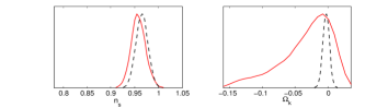
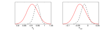
Figure 2: 1-D marginal posterior distributions for different power spectrum parameter models: PL 1 ($n_{\rm s}$; top row), PL 2 ($n_{\rm s}+\Omega_{k}$; middle row) and PL 3 ($n_{\rm s}+n_{\rm run}$; bottom row), using dataset 1 (solid line) and dataset 2 (dashed line).

In Fig 2 we plot the 1-D marginal posteriors for the power spectrum parameters in each of the power-law models, using both dataset 1 and dataset 2. We now on refer to the mean of the posterior distribution of each parameter together with its 68 % confidence interval. For model 1 ($n_{\rm s}$), we see that scale-invariant spectrum $n_{\rm s}=1$ is ruled out, as expected, with high confidence level using either dataset. Indeed, the constraints on $n_{\rm s}$ for a flat universe (PL 1) and a curved universe (PL 2) using dataset 2 are similar: $n_{\rm s}=0.963\pm 0.011$ and $n_{\rm s}=0.965\pm 0.012$ respectively. The inclusion of the running parameter (PL 3) displaces and broadens the posterior probability, such that $n_{\rm s}=0.944\pm 0.020$.

When the curvature is considered as a free parameter, dataset 1 selects a closed universe $\Omega_{k}=-0.033^{+0.030}_{-0.041}$ with a Hubble constant $H_{0}=61.0^{+12.2}_{-12.5}$ km/s/Mpc. Similarly, for a flat Universe the constraints for the running parameter $n_{\rm run}=-0.038\pm 0.027$ and $H_{0}=66.6\pm 3.8$ km/s/Mpc are in good agreement with Larson et al. (2011). The inclusion of measurements on different scales (dataset 2) weakens the geometric degeneracy and tightens significantly the constraints, yielding a mean posterior value for the curvature $\Omega_{k}=-0.0026\pm 0.0049$ and Hubble parameter $H_{0}=70.4\pm 1.7$ km/s/Mpc. On the other hand, we observe the best-fit for the running parameter is moved closer to its zero value with constraints $n_{\rm run}=-0.018\pm 0.016$

In Fig 3, we plot the reconstructed shape for the power spectrum for the simple spectral index in a curved universe and the running parameterisation in flat universe, using mean values of the posterior distributions found from dataset 2.

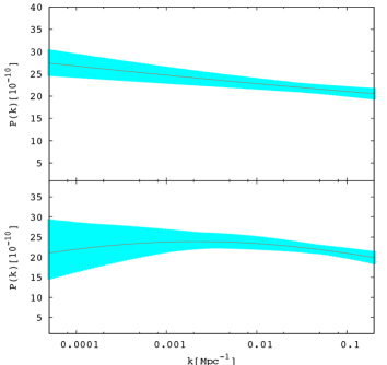
Figure 3: Primordial power spectrum reconstructed using mean values of the posterior distributions found from dataset 2, for PL model 2 ($n_{\rm s}+\Omega_{k}$; top panel) and PL model 3 ($n_{\rm s}+n_{\rm run}$; bottom panel), with $1\sigma$ error bands.

5.2 LD model

We choose to describe the LD spectrum in terms of the parameters $b_{0}$ and $b_{4}$, letting $\mu$ be a derived parameter such that the conformal time constraint is fulfilled. The resulting constraints from dataset 2 on the parameters describing the LD power spectrum are shown in Fig 4.

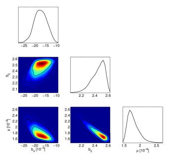
Figure 4: Marginalised 1D and 2D probability distributions for the power spectrum parameters $b_{4}$, $b_{0}$ and $\mu$ in the LD model, using dataset 2. 2D constraints are plotted with $1\sigma$ and $2\sigma$ confidence contours.

In particular we obtain the constraint $b_{0}=2.45^{+0.90}_{-0.11}$, which is intimately linked to the number of $e$-folds $N$ during the inflationary epoch through (19). We also find the constraint $b_{4}\,[10^{-9}]=-17.74^{+2.92}_{-2.78}$ and we note the effect occurring through (21): a greater initial curvature (increased $|b_{4}|$) would drive the universe today closer to be flat (decrease $|\Omega_{k}-1|$). Finally, the constraint on the scalar field mass is $\mu\,[10^{-6}]=1.79^{+0.17}_{-0.16}$.

The LD model requires a closed universe, then using dataset 2 a very small value for the curvature parameter is obtained $\Omega_{k}=-0.43^{+0.27}_{-0.28}\times 10^{-2}$, together with a Hubble constant of $H_{0}=68.9\pm 1.3$ km/s/Mpc, both of which are compatible with all existing observations. We note, however, that many authors have argued on the difficulty to construct realistic closed-universe models with the required number of $e$-folds and also that a fine tuning might arise from the initial conditions to obtain an homogeneous universe after inflation (Ellis et al. 2002; Linde 2003; Uzan et al. 2003). In this sense, the LD model provides the correct order of magnitude in the prediction of the number of $e$-folds given by $N=48.1^{+3.3}_{-4.2}$ (see Fig 5).

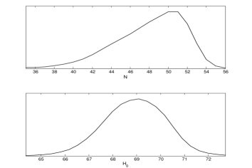
Figure 5: Marginalised 1D probability distributions for the number of e-foldings produced during inflation (top) and Hubble constant (bottom), obtained from the LD model using dataset 2.

Finally, we plot in Fig. 6 the reconstructed primordial power spectrum for the LD model together with $1\sigma$ error bands. It is worth pointing out that the LD spectrum automatically contains a clear cut-off at low $k$-values and an additional fall-off at high wavenumber. A low-$k$ truncation of the primordial spectrum of this type was proposed phenomenologically by Efstathiou (2003). This kind of behaviour could be responsible for the small CMB power currently observed at low $l$ multipoles.

Figure 6: Primordial power spectrum reconstructed from the LD model using mean values of the posterior distributions obtained from dataset 2, with $1\sigma$ error bands.

6 Model selection

We now investigate which model provides the best description of the data by performing model selection based on the value of the Bayesian evidence. Before performing this process on the real datasets, however, we first test our approach by applying it to an idealised dataset.

6.1 Application to simulated data

Figure 7: Top (bottom) panel shows a simulated CMB temperature (polarisation) power spectrum, convolved with chi-square noise and limited data up to $l$ of 2000. The model from which it was produced is drawn by the blue line.

To test our model selection (and parameter estimation) method, we implement the LD spectrum in a modified version of the CAMB package (Lewis et al. 2000) to simulate the CMB power spectrum predicted by the LD model using standard values for the cosmological parameters, i.e. those obtained from WMAP7. The predicted temperature and E-mode polarisation CMB spectra are plotted as the dashed line in Fig. 7. We simulate an idealised process where only cosmic variance noise was added to the spectra such that each $C_{l}$ value becomes a random variable drawn from a $\chi^{2}_{2l+1}$ distribution with variance

$$(\Delta C_{l})^{2}=\frac{2}{2l+1}C_{l}^{2}.$$ (26)

The 1D marginalised parameter constraints for the LD model resulting from the analysis of this simulated dataset are shown in Figure 8. We observe that our approach yields constraints that appear consistent, within statistical error, with the input values used in the simulation, which are indicated by the vertical lines in each plot. Moreover, these results give us an indication of how accurately the parameters of the LD model can be constrained with an optimal CMB dataset. In particular, we note that the behaviour of the posterior for $\Omega_{k}$ is reflected in that obtained for $b_{4}$, that is because of the link between them through the see-saw mechanism.

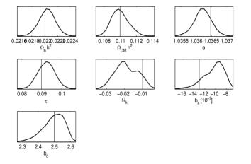
Figure 8: 1-D marginalised parameter constraints for a simulated model. The set of parameters used to construct the mock data is represented by the vertical lines. The $y$-axis is relative probability.

The evidence values of the models considered for the primordial spectrum are given in Table 3. Based on Jeffreys’ criterion we observe significant difference in the log-evidences for each model. Thus, there is a clear distinction between models, with the data clearly indicating a preference, as expected, for the LD model used to generate the simulated data. Given the success of model selection on simulated data, we now turn to real data with some confidence.

Table 3: Difference of log-evidences for the different parameterisations relative to simple power-law flat model for the simulated CMB dataset.

Model	$\Delta\ln\mathcal{Z}$
PL 1 ($n_{\rm s}$)	0.0   $\pm$   0.4
PL 2 ($n_{\rm s}$ + $\Omega_{k}$)	-1.0   $\pm$   0.4
PL 3 ($n_{\rm s}$ + $n_{\rm run}$)	-3.1   $\pm$   0.4
LD model	+3.7   $\pm$   0.4

6.2 Application to real data

Before performing the Bayesian selection between our different models for the primordial power spectrum, we will momentarily use a frequentist method and compute the goodness-of-fit of each of the models using real data. Using the best-fit parameters obtained for each model with dataset 1, we may calculate $\chi^{2}_{\rm min}$, defined as $-2\ln\mathcal{L}_{\rm max}$, at the maximum point in each case. These values are given in Table 4 from which we see that all three models fit the data almost equally as well.

Table 4: Log-likelihood values at the best-fit point for three different models of the primordial power spectrum using dataset 1.

Model	$N_{\rm params}$	-$\ln\mathcal{L}_{max}$
PL 2 ($n_{\rm s}$ + $\Omega_{k}$)	7	7475.3
PL 3 ($n_{\rm s}$ + $n_{\rm run}$)	7	7473.5
LD model	7	7473.0

Turning now to Bayesian model selection, the difference in the log-evidences for each of the models are given in Table 5, as derived from dataset 1 and dataset 2 respectively.

Table 5: Difference of log-evidences for each of our models for the primordial power spectrum, relative to the simple power-law model.

Model	$N_{\rm params}$	Dataset 1	Dataset 2
PL 1 ($n_{\rm s}$)	6	0.0 $\pm$ 0.3	0.0 $\pm$ 0.3
PL 2 ($n_{\rm s}$ + $\Omega_{k}$)	7	$-0.5$ $\pm$ 0.3	$-2.6$ $\pm$ 0.3
PL 3 ($n_{\rm s}$ + $n_{\rm run}$)	7	$-0.8$ $\pm$ 0.3	$-1.7$ $\pm$ 0.3
LD model	7	$+1.2$ $\pm$ 0.3	$-0.9$ $\pm$ 0.3

The log-evidence difference should be interpreted in the context of the Jeffreys’ scale given in Table 1. In the analysis we have considered a wide conservative prior for the parameters in each model. The parameter estimation results in Section 5 showed that the constraints obtained lie well within our chosen prior and as such any increase in the prior would not include very much more posterior mass within the evidence integral. Thus we would not expect reasonable modifications of the prior range to alter the results makedly.

For dataset 1, the similarity in log-evidences and their statistical uncertainties make it difficult to obtain definitive conclusions. When the evidence values are ranked, however, we observe a slight preference in favour of the LD spectrum over the three power-law parameterisations, whereas model 3 ($n_{\rm s}+n_{\rm run}$) is significantly the most disfavoured. The inclusion of additional information on different scales with dataset 2 significantly reduces the evidence for the three 7-parameter models. We notice that a curved universe with a simple power-law, PL 2 ($n_{\rm s}+\Omega_{k}$), is strongly disfavoured relative to a flat universe with a power-law spectrum ($n_{\rm s}$). When we perform a comparison of models which contain the same number of parameters, we observe the LD model is 1.7 units of log-evidence above the PL model 2, which is a significant difference, but only 0.8 log-units above PL model 3. The $\Lambda$CDM model with a power-law spectrum has the largest evidence in this case. We observe from Table 5, that from all of the models considered with equal numbers of parameters (with either dataset) that the LD model is currently preferred.

7 Discussion and Conclusions

The novel closed universe model proposed by Lasenby $\&$ Doran gives rise to a boundary condition on the total available conformal time:

$$\eta_{M}+\eta_{I}=\frac{\pi}{2}.$$

Here we have split the universe evolution in two main epochs that contribute to the amount of conformal time: matter-dominated epoch and inflationary period. The matter epoch can be described in terms of matter-energy content of the universe: baryons ($\Omega_{\rm b},$), photons ($\Omega_{\rm r}$), Cold dark matter ($\Omega_{\rm DM}$) and dark energy ($\Omega_{\Lambda}$), as well as on its expansion history: Hubble time ($H_{0}$). The inflationary period is encoded in three parameters that have emerged in the construction of the appropriate initial conditions. They are related to the initial curvature ($b_{4}$), the initial expansion size of the universe ($b_{0}$) and the amplitude of perturbations ($\mu$). Such parameters are not predicted a priori, rather we have fit them using current observational data. Notice that we have the freedom to pick two of them and compute the third parameter through the constraint imposed on the conformal time. In this paper we have focused on $b_{0}$ and $b_{4}$ to describe the LD spectrum. The comparison of the best-fit primordial spectra for our different models is shown on Fig 9.

We test the LD spectrum by building a simple toy model from a chosen CMB spectrum with simulated cosmic variance noise. A full Bayesian analysis was performed for this toy model and various parameterisations of the primordial power spectrum. We have included not only the estimation of cosmological and spectral parameters but also the Bayesian evidence. For real data, we compared the $\chi^{2}$ for the three different models and concluded that the goodness-of-fit for the LD model is about the same as the well-studied power-law models. We also pointed out that the constraints on the cosmological parameters in the LD model are consistent within $1\sigma$ error bars with the power-law models, as shown in Figs 10 and 11.

Figure 9: Primordial and anisotropy power spectrum for different models of the primordial spectrum: $n_{\rm s}$ (dotted line), $n_{\rm s}+\Omega_{k}$ (dash-dot line), $n_{\rm s}+n_{\rm run}$ (dashed line) and LD model (solid line), using the best-fit parameter values for dataset 2.

The Lasenby $\&$ Doran model predicts a primordial scalar spectrum that at large scales naturally incorporates a drop off without the need to parameterise it, while, at small scales it automatically incorporates a degree of negative running compared with the standard power law parameterisation (see e.g. Fig 9 below or Fig. 17 in Lasenby $\&$ Doran, 2005, for a visual comparison). Given that the primordial parameters $b_{0}$ and $b_{4}/\mu^{4/3}$ are well constrained and of order unity, no fine tuning is needed for the construction of the initial conditions. Moreover, the LD model has the required order of $e$-foldings to obtain realistic models of a closed inflationary universe. Finally, even though the Bayesian evidence from each model showed that it is difficult to make definitive conclusions because of the presence of statistical uncertainties, an important result to emphasise is that for the models with the same number of parameters, the preferred model to explain current cosmological observations in given by the LD model. This may be seen by noting that, for models with 7 parameters, Table 5 shows that the LD model is preferred significantly (by 1.7-2.0 $\log$ units of evidence) in all cases except relative to $n_{\rm s}+n_{\rm run}$ with dataset 2, for which it is preferred by 0.8 $\log$ units.

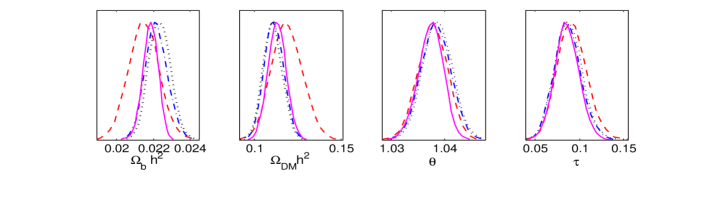
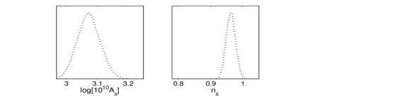
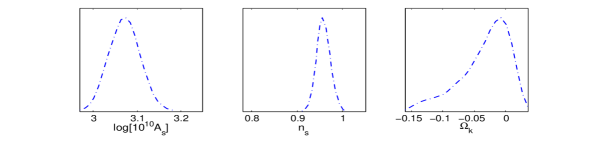
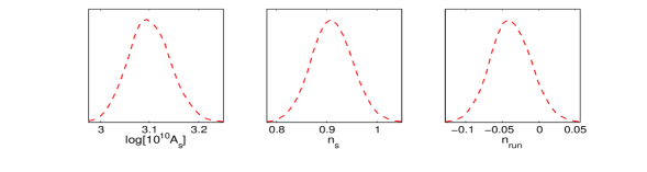
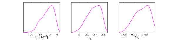
Figure 10: Marginalised parameter constraints corresponding to $n_{\rm s}$ (dotted line), $n_{\rm s}+\Omega_{k}$ (dash-dot line), $n_{\rm s}+n_{\rm run}$ (dashed line) and L & D model (solid line), using dataset 1.

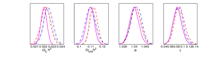
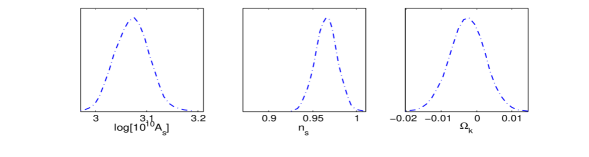
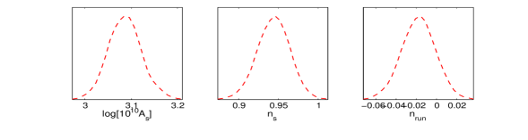
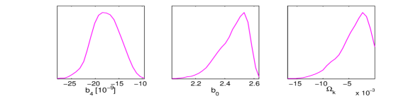
Figure 11: Marginalised parameter constraints corresponding to $n_{\rm s}$ (dotted line), $n_{\rm s}+\Omega_{k}$ (dash-dot line), $n_{\rm s}+n_{\rm run}$ (dashed line) and L & D model (solid line), using dataset 2.

References

- Albrecht & Steinhardt (1982) Albrecht A., Steinhardt P. J., 1982, Phys. Rev. Lett., 48, 1220
- Barriga et al. (2001) Barriga J., Gaztanaga E., Santos M., Sarkar S., 2001, MNRAS, 324, 977
- Bayes (1761) Bayes T., 1761, Phil. Trans. R. Soc., 370
- Beltrán et al. (2005) Beltrán M., García-Bellido J., Lesgourgues J., Liddle A. R., Slosar A., 2005, Phys. Rev. D, 71, 063532
- Bridges et al. (2009) Bridges M., Feroz F., Hobson M. P., Lasenby A. N., 2009, MNRAS, 400, 1075
- Bridges et al. (2006) Bridges M., Lasenby A. N., Hobson M. P. 2006, MNRAS, 369, 1123
- Bridges et al. (2007) Bridges M., Lasenby A. N., Hobson M. P., 2007, MNRAS, 381, 68
- Bridle et al. (2003) Bridle S. L., Lewis A. M., Weller J., Efstathiou G., 2003, MNRAS, 342, L72
- Contaldi et al. (2003) Contaldi C. R., Peloso M., Kofman L., Linde A., 2003, JCAP, 2003, 002
- Efstathiou (2003) Efstathiou G., 2003, MNRAS, 343, L95
- Ellis et al. (2002) Ellis G. F. R., McEwan P., Stoeger W., Dunsby P., 2002, Gen. Rel. Grav., 34, 1461
- Feroz et al. (2009) Feroz F., Hobson M. P., Bridges M., 2009, MNRAS, 398, 1601, code at http://www.mrao.cam.ac.uk/software/ multinest/downloads.html
- Feroz et al. (2008) Feroz F., Hobson M. P., 2008, MNRAS, 384, 449
- Guo et al. (2011) Guo Z. K., Schwarz D. J., Zhang Y. Z., arXiv:1105.5916
- Guth (1981) Guth A. H., 1981, Phys. Rev. D, 23, 347
- Hannestad (2004) Hannestad S., 2004, JCAP, 2004, 002
- Hlozek et al. (2011) Hlozek R., arXiv:1105.4887
- Hobson et al. (2002) Hobson M. P., Bridle S., Lahav O., 2002, 335, 377
- Jeffreys (1961) Jeffreys H., 1961, Theory of Probability. Oxford
- Jones et al. (2006) Jones, W. C., et al., 2006 ApJ, 647, 823
- Komatsu et al. (2011) Komatsu E., et al., 2011, ApJ Supplement Series, 192, 18
- Kuo et al. (2004) Kuo C. L., et al., 2004, ApJ, 600, 32
- Larson et al. (2011) Larson D., et al., 2011, ApJ Supplement Series, 192, 16
- Lasenby (2003) Lasenby A., http://www.mrao.cam.ac.uk/~clifford /publications/abstracts/anl_ima2002.html
- Lasenby & Doran (2004) Lasenby A., Doran C., 2004, AIP Conference Proceedings, 736, 53
- Lasenby & Doran (2005) Lasenby A., Doran C., 2005, Phys. Rev. D, 71, 063502
- Lewis & Bridle (2002) Lewis A., Bridle S., 2002, Phys. Rev. D, 66, 16, code at http://cosmologist.info/cosmomc/
- Lewis et al. (2000) Lewis A., Challinor A., Lasenby A., 2000, ApJ, 538, 473, code at http://camb.info/
- Liddle (2004) Liddle A. R., 2004, MNRAS, 351, L49
- Liddle (2007) Liddle A. R., 2007, MNRAS Letters, 377, L74
- Liddle (2006) Liddle A. R., Mukherjee P., Parkinson D., A&G, 47, 4.30
- Liddle & Lyth (1999) Liddle A. R., Lyth D. H., 1999, Cosmological Inflation and Large Scale Structure, Cambridge University Press, Cambridge
- Linde (2003) Linde A., 2003, JCAP, 2003, 002
- Mukhanov & Chibisov (1982) Mukhanov V. F., Chibisov G. V., 1982, Sov. Phys. JETP, 56
- Mukherjee et al. (2006) Mukherjee P., Parkinson D., Liddle A. R., 2006, ApJ Letters, 638, 258
- Peiris & Verde (2010) Peiris H. V., Verde L., 2010, Phys Rev D, 81, 021302
- Readhead et al. (2004) Readhead A. C. S., et al., 2004, ApJ, 609, 498
- Reid et al. (2010) Reid B. A., et al., 2010, MNRAS, 404, 1365
- Riess et al. (2009) Riess A. G., et al., 2009, ApJ, 699, 539
- Shaw et al. (2007) Shaw J. R., Bridges M., Hobson M. P., 2007, MNRAS, 378, 1365
- Skilling (2004) Skilling J. 2004, AIP Conference Proceedings, 735, 395
- Trotta (2007) Trotta R., 2007, MNRAS, 378, 72
- Trotta (2008) Trotta R., 2008, Contemporary Physics, 49, 71
- Uzan et al. (2003) Uzan J. P., Kirchner U., Ellis G. F. R., 2003, MNRAS, 344, L65
- Verde & Peiris (2008) Verde L., Peiris H., 2008, JCAP, 2008, 009