Motion around a Monopole $+$ Ring system:
I. Stability of Equatorial Circular Orbits vs
Regularity of Three-dimensional Motion.

Abstract

We study the motion of test particles around a center of attraction represented by a monopole (with and without spheroidal deformation) surrounded by a ring, given as a superposition of Morgan & Morgan discs. We deal with two kinds of bounded orbits: (i) Equatorial circular orbits and (ii) general three-dimensional orbits. The first case provides a method to perform a linear stability analysis of these structures by studying the behavior of vertical and epicyclic frequencies as functions of the mass ratio, the size of the ring and/or the quadrupolar deformation. In the second case, we study the influence of these parameters in the regularity or chaoticity of motion. We find that there is a close connection between linear stability (or unstability) of equatorial circular orbits and regularity (or chaoticity) of the three-dimensional motion.

1 Introduction

Light particles interacting with a central massive body are frequently encountered in diverse fields of physics. Electrons in rotating molecules and particular versions of the many-body problem in celestial mechanics are the most well-known examples, but some nuclear models fall into the same category. Increasing amounts of information about narrow planetary rings suggest that such rings are often associated with the so-called shepherd satellites (Goldreich & Tremaine 1979 ), and may exist due to mechanisms somewhat more complicated than the well known broad rings (Greenberg & Brahic 1984 ; Smith et al. 1981 ; Smith et al. 1982 ; Murray et al. 2005 ).

Recent progress in the subject suggest a generic mechanism, that does not depend on Kepler orbits, to explain the formation of rings around a rotating object which also holds for systems quite different from planetary rings. In rotating scattering systems, the generic saddle-center scenario leads to stable islands in phase space. Non-interacting particles whose initial conditions are defined in such islands will be trapped and form rotating rings. This result is generic and guarantees that the orbits supporting the ring structure are rather insensitive to small perturbations and thus may play a role in different situations of the type mentioned above (Benet & Seligman 2000 ). So, although we are interested in studying planetary rings, there are many other systems that exhibit the same structure and therefore one can perform similar treatments by knowing the nature of the forces involved.

Now then, based on the arguments mentioned above, one may conjecture that once the ring structure is formed around the rotating body, it remains stable, as revealed by the structure of its phase space. In this set of papers, we propose an analytical study about the dynamical aspects concerning the stability of ring structures and the relation with the existence of isolated islands in the phase space. In this first paper we focus in the effects related to the physical parameters like the mass of the central body, the geometry of the central body, the mass of the ring and the size of the ring. In next papers, we plan to examine the influence of the angular momentum of the system in its stability, as well as, large perturbations like the interaction with external satellites and their responses to resonance.

Planetary rings consist in thin discs of cosmic dust and other small colliding particles revolving around a central planet in a flat disc-shaped region. The most spectacular example of ring structures are those around Saturn (Porco et al. 2005 ; Cuzzi et al. 2010 ), but they are a common feature of the other three gas giants of the solar system; Jupiter, Uranus and Neptune possess ring systems of their own. Recent reports have suggested that the Saturnian moon Rhea may have its own tenuous ring system, which would make it the only moon known to possess a ring system (Jones et al. 2008 ).

There are many possible mechanisms to explain the existence of planetary rings, but essentially three of them are the most relevant: from material of the protoplanetary disc that was within the Roche limit of the planet and thus could not coalesce to form moons; from the debris of a moon that was disrupted by a large impact; or from the debris of a moon that was disrupted by tidal stresses when it passed within the planet’s Roche limit. This last one allows us to predict that Phobos, a moon of Mars, will break up and form into a planetary ring in about 50 million years due to its low orbit (Holsapple 2001 ).

Additionally, we should take into account the increasing amount of data we get from extrasolar systems. The discovery of extrasolar planets (which up to date are more than 300) by radial velocity measurements has provided the first dynamical characteristics of planets: orbital elements and mass. The next step will be to investigate physical characteristics: albedo, temperature, radius, etc, and their surroundings. Among the latter are planetary rings. The emitted thermal infrared light from the planet should show no phase effect assuming the planet is in thermal equilibrium. But the reflected visible light will vary with phase angle, as should be shown by a broad-band photometric follow-up of the planet during its orbital motion. In particular, it has been studied from different perspectives how the presence of a ring around a planet would influence its brightness as a function of its orbital position and based on that there have been multiple theoretical predictions for photometric and spectroscopic signatures of rings around transiting extrasolar planets (Barnes & Fortney 2004 ; Arnold & Schneider 2006 ; Ohta, Taruya and Suto 2009 ). So, understanding the dynamics of composed planetary systems would not constitute just an astrophysical curiosity, it would have some impact on the strategy for their detection (see Arnold and Schneider 2004 and the references therein).

On the other hand, it has been shown that collisions play an important role in the dynamical aspects of the rings (Longaretti 1992 ; Sicardy 2006 ). Under some physical assumptions, one can see that as this process dissipates mechanical energy, while conserving angular momentum of the ensemble, tend to flatten the disc perpendicular to its total angular momentum, and to circularize the particles orbits. If the planet is not spherically symmetric, as it is the case for all the oblate giant planets, apart of being flat the configuration becomes a equatorial ring. Of course, some physics is still missing in the description of the rings and an interesting question here would be if these effects that one does not take into account as a first approximation are relevant in the dynamics of the ring. A classical approach is to consider what happens to the system when small perturbations are applied.

Commonly, disc-like systems such as planetary rings are described by a set of coupled equations: two hydrodynamic equations (Euler’s and continuity equation), Poisson’s equation and a equation of state (Toomre 1964 ; Binney & Tremaine 2008 ). For small enough disturbances, these equations can be linearized and solved under further simplifications as there are still missing analytical self-consistent models of planetary rings. Nevertheless, it is possible to obtain useful information of this by using simplified models which illustrates quantitatively how pressure and rotation tend to stabilize the disc against self-gravity.

Although most rings were thought to be unstable and to dissipate over the course of tens or hundreds of millions of years, recent evidence coming from NASA’s Cassini-Huygens Mission suggest that Saturn’s rings might be quite old, dating to the early days of the Solar system. Then, the exact mechanism to explain which physical factors account for the stability of these systems is still an open question to be answered.

Our approach to study the stability of rings will be quite different of the mentioned above. The method we will use is insensible to the hydrodynamical aspects of the rings but with the advantage that we will have under control the geometrical aspects of the models, namely the size and shape of the ring, the mass quotient between the planet and the ring and deviations from the spherical geometry of the planet. Also, similar techniques can be applied to study the effects caused by the angular momentum of the planet and even the influence of external satellites, but these topics are out of the aim of this paper and will be left for future works. Another benefit of this approach is that it becomes easy to elucidate a non-trivial connection between the stability in equatorial circular orbits and the regularity in three-dimensional motion. In particular, we will see how the existence of isolated islands will lead to stable ring configurations and how relevant are the physical parameters mentioned above.

Now then, the exact gravitational potential of a ring of zero thickness and constant linear density is given in its exact form by an elliptic integral that is seldom used for practical purposes. This potential is usually approximated by truncated series of spherical harmonics, i.e., a multipolar expansion (see for example the deep analysis of orbits performed in Tresaco & Ferrer 2010 ). As far as we know there are not simple expressions for the exact gravitational potential of a finite flat ring with inner and outer edges and any surface density.

Meanwhile, simple potential-density pairs for thin discs are known. The simpler is the Plummer-Kuzmin disc (Kuzmin 1956 ) that represents a simple model with a concentration of mass in its center and density that decays as $1/r^{3}$ on the plane of the disc. This structure has no boundary even though for practical purposes one can put a cutoff radius wherein the main part of the mass is inside, say 98% of the mass. There are many other models in the literature (Lynden-Bell 1962 ; Mestel 1963 ; Toomre 1963 ; Hunter & Toomre 1969 ; Kalnajs 1972 ; Jiang 2000 ; Jiang & Moss 2002 ; González & Reina 2006 ; Jiang & Ossipkov 2007 ; Pedraza, Ramos-Caro & González 2008 ), some of them of infinite extension but others with an outer edge. Among the last ones, a family of simple models are the Morgan and Morgan discs (Morgan & Morgan 1969 ), which has been inverted (Lemos & Letelier 1994 ) in order to obtain infinite discs with a central hole of the same radius of the original disc. We can also put a cutoff in these structures and therefore the inverted Morgan and Morgan discs can be considered as representing a flat rings. These models have been used by the authors in order to study the superposition of an annular disk with a central black hole in the context of the General Theory of Relativity (see also Semerák & Suková 2010 ; Lora-Clavijo, Ospina-Henao & Pedraza 2010 , for recent related works).

Another approach to construct flat ring structures is by the superposition of different kind of discs. In Letelier 2007 the author superposed Morgan and Morgan discs (Morgan & Morgan 1969 ) while in Vogt & Letelier 2009 the Kuzmin-Toomre discs (Kuzmin 1956 ; Toomre 1963 ) were used. In this paper we will use the first of the above models which are relatively simple and superposing the potential of the planet will allow us to study the effects of those parameters we have been talking about.

2 Models of rings around a spherically symmetric object

In this section we shall focus on simple analytical models that represent sources conformed by an axisymmetric thin ring and a central object that we will assume with spherical symmetry, i.e. a body characterized only by its monopolar moment. The effects concerning with oblate or prolate deformation of the center of attraction, i.e. the inclusion of a quadrupolar moment, will be studied in the last section.

In a recent work, Letelier 2007 , shows how to construct a simple family of potential-density pairs for flat rings by means of the superposition of Morgan and Morgan discs (Morgan & Morgan 1969 ). These discs are finite in extension and have a well-behaved surface mass density with a maximum in the center and monotonically decreasing up to the edge. The structures obtained by the superposition of discs with different densities have a finite outer radius and zero density on their centers, i.e. discs with a hole in their centers, or in other words flat rings. Although the models do not have an inner edge, for practical purposes one can put a cutoff radius and neglect the residual density (which becomes smaller for higher members of the family).

The Morgan & Morgan discs are obtained by solving the Laplace equation in the natural coordinates to represent the gravitational potential of a disc-like structure, i.e. oblate coordinates $(\xi,\eta,\varphi)$ (defined in the ranges $0\leq\xi<\infty$ and $-1\leq\eta\leq 1$) that are related to the usual cylindrical coordinates $(R,z,\varphi)$ by

$$\begin{split}R&=a\sqrt{(\xi^{2}+1)(1-\eta^{2})},\\ z&=a\xi\eta,\end{split}$$ (1)

where $a$ is a positive constant defining the disc radius. The inverse relations are given by

$$\begin{split}a\xi&={\rm Re}\left[\sqrt{R^{2}+(z-ia)^{2}}\right],\\ a\eta&=-{\rm Im}\left[\sqrt{R^{2}+(z-ia)^{2}}\right].\end{split}$$ (2)

Note that, according to (1), on the equatorial plane $z=0$ one has to distinguish between two regions: (i) the points inside the disc, with coordinates $\xi=0$ and $\eta\leq\sqrt{1-R^{2}/a^{2}}$; (ii) the points outside the disc, with coordinates $\eta=0$ and $\xi>\sqrt{R^{2}/a^{2}-1}$.

The mass surface density of each disc (labeled with the positive integer $n$) is given by

$$\Sigma_{n}(R)=\frac{(2n+1)M_{n}}{2\pi a^{2}}\left(1-\frac{R^{2}}{a^{2}}\right)^{n-1/2},$$ (3)

where $M_{n}$ is the total mass and $a$ the disc radius. Such mass distribution generates an axially symmetric gravitational potential, that can be written as

$$\hat{\Phi}_{n}(\xi,\eta)=-\sum_{k=0}^{n}A_{2k,2n}q_{2k}(\xi)P_{2k}(\eta).$$ (4)

Here, $P_{2k}(\eta)$ and $q_{2k}(\xi)=i^{2k+1}Q_{2k}(i\xi)$ are the usual Legendre polynomials and the Legendre functions of the second kind respectively, and $A_{2k,2n}$ are constants given by

$$A_{2k,2n}=\frac{M_{n}G\pi^{1/2}(4k+1)(2n+1)!}{a2^{2n+1}(2k+1)(n-k)!\Gamma(n+k+3/2)q_{2k+1}(0)},$$ (5)

where G is the gravitational constant. If we consider discs of the same radius $a$ and decreasing mass,

$$M_{n}=\frac{2\pi\Sigma_{c}a^{2}}{2n+1},$$ (6)

where $\Sigma_{c}$ is a constant that will be taken equal for all discs of the Morgan and Morgan family, we obtain discs with surface density

$$\Sigma^{\prime}_{n}=\Sigma_{c}\left(1-\frac{R^{2}}{a^{2}}\right)^{1/2}\left(1-\frac{R^{2}}{a^{2}}\right)^{n-1}.$$ (7)

In order to obtain a mass density in agreement with a flat ring distribution, Letelier 2007 considered the superposition

$$\begin{split}\tilde{\Sigma}_{n}&=\sum_{k=0}^{n}\frac{n!(-1)^{n-k}}{(n-k)!k!}\Sigma^{\prime}_{n+1-k},\\ &=\Sigma_{c}\left(1-\frac{R^{2}}{a^{2}}\right)^{1/2}\frac{R^{2n}}{a^{2n}}.\end{split}$$ (8)

Figure 1: The mass surface density for the first ten members of the ring family constructed as a superposition of Morgan and Morgan discs.

We have that the above superpositions give rings of radius $a$ and a central residual density that becomes smaller for larger $n$. For practical purposes one can put a cutoff inner radius $b_{n}$, which we will take as the radius such that the density falls below the 1% of its maximum. In table 1 we show the values of $b_{n}/a$ for the first ten members of this family and, in figure 1, their corresponding mass surface densities. The total mass of each ring is

$$\begin{split}\tilde{M}_{n}=&\;\frac{2\pi\Sigma_{c}}{a^{2n}}\int_{0}^{a}\left(1-\frac{R^{2}}{a^{2}}\right)^{1/2}R^{2n+1}dR,\\ =&\;\frac{\pi^{3/2}a^{2}\Sigma_{c}\Gamma(n+1)}{2\Gamma(n+5/2)}.\end{split}$$ (9)

Thus by increasing $n$, the mass of the flat ring decreases along with the size of the region where it is distributed (near the outer radius). Note that this is a feature associated to the particular family of models we are considering, not with the corresponding physical applications. The values of $n$ and $\Sigma_{c}$ are inferred from basic data corresponding to a special case. For example, to describe a ring with mass $6\times 10^{18}$Kg, inner radius $122000$Km and outer radius $137000$Km, we have to set $n=28$ and $\Sigma_{c}\approx 1800g/cm^{2}$, leading to to a maximum mass density of about $40g/cm^{2}$ (these values agree roughly with the measurements of the so-called Ring A of Saturn (Dougherty et al. 2009 )).

The potentials associated to these structures can be obtained using a superposition with the same coefficients as the ones used for the densities, i.e.,

$$\tilde{\Phi}_{n}=\sum_{k=0}^{n}\frac{n!(-1)^{n-k}}{(n-k)!k!}\Phi^{\prime}_{n+1-k},$$ (10)

where $\Phi^{\prime}_{n}$ is the same as $\hat{\Phi}_{n}$ with the masses given by equation (6).

$n$ $b_{n}/a$ 1 0.06210 2 0.23292 3 0.36991 4 0.43940 5 0.54302

$n$ $b_{n}/a$ 6 0.59222 7 0.64335 8 0.67884 9 0.70798 10 0.73231

Table 1: Values of the ratio $b_{n}/a$ for the first ten members of the family of rings given by the mass surface (8). Here $b_{n}$ represents the inner cut-off radius and $a$ is the outer radius. For higher members of the family the mass concentration tends to be located near the outer edge.

Finally we add a monopolar term, which represents the exterior field of a central spherically symmetric object, to the ring potential described above. Thus, the total gravitational potential reads

$$\Phi_{n}=\tilde{\Phi}_{n}-\frac{GM_{p}}{\sqrt{R^{2}+z^{2}}},$$ (11)

where $M_{p}$ is the mass of the central object. Although our 4-parametric toy model is quite simple, we believe that this is a good starting point to study the effects on the dynamics caused by the mass ratio $\tilde{M}_{n}/M_{p}$ and the radius ratio $a/b_{n}$ which is one of the purposes of this paper. The effects caused by the rotation of the central body (its own angular momentum would be an additional parameter), will be studied in a next paper through the post-Newtonian scheme.

3 MOTION OF TEST PARTICLES

Let us deal with the problem of motion of test particles around the models described above. Since $\Phi_{n}$ is static and axially symmetric, the specific energy $E$ and the specific axial angular momentum $\ell$ are conserved along the particle motion, which is restricted to a three dimensional subspace of the $(R,z,V_{R},V_{z})$ phase space. Each orbit is determined by the set of equations (Binney & Tremaine 2008 )

$$\dot{R}={V}_{R}, \qquad\dot{z}={V}_{z},$$ (12a)

$$\dot{V}_{R}=-\frac{\partial\Phi_{n}^{*}}{\partial R}, \qquad\dot{V}_{z}=-\frac{\partial\Phi_{n}^{*}}{\partial z},$$ (12b)

where $\Phi^{*}_{n}$ is the effective potential, defined by

$$\Phi^{*}_{n}=\Phi_{n}+\frac{\ell^{2}}{2R^{2}},$$ (13)

in terms of which the particle’s energy can be written as

$$E=\frac{1}{2}({V}_{R}^{2}+{V}_{z}^{2})+\Phi^{*}_{n}.$$ (14)

Relations (12a)-(12b) define an autonomous system whose equilibrium points are $V_{R}=V_{z}=z=0$ and $R=R_{c}$, where $R_{c}$ must satisfy the equation

$$\left(\frac{\partial\Phi^{*}_{n}}{\partial R}\right)_{(R_{c},0)}=-\frac{\ell^{2}}{R_{c}^{3}}+\left(\frac{\partial\Phi_{n}}{\partial R}\right)_{(R_{c},0)}=0,$$ (15)

that is the condition for a circular orbit in the plane $z=0$. In other words, the equilibrium points of the system occur when the test particle describes equatorial circular orbits of radius $R_{c}$, specific energy $E=\Phi^{*}_{n}(R_{c},0)$, and specific axial angular momentum given by

$$\ell_{c}^{2}=R_{c}^{3}\left(\frac{\partial\Phi_{n}}{\partial R}\right)_{(R_{c},0)}\>\>.$$ (16)

The description of circular orbits in the equatorial plane is a first step to understand the linear stability of the system, as well as, the regularity or chaoticity of three dimensional orbits. On the one hand, if one assumes as a first approximation that the structures are built from particles moving only in circular orbits, the epicyclic and vertical frequencies of quasi circular orbits provide us a criterion for the system’s stability (see section 4). On the other hand, the analysis of such frequencies also leads to determine the existence of saddle points, which are preliminary indicators of irregular motion.

In order to deal with the problem of correlation between regularity of three dimensional motion and the stability of circular orbits, we have to distinguish between exterior and interior motions of test particles, separately. As we pointed out in the last section, the relation between oblate and cylindrical coordinates is given by (2) or, in a more explicit form

$$\begin{split}\xi&=\Delta(R,z)\cos\left[\Theta(R,z)\right],\\ \eta&=\Delta(R,z)\sin\left[\Theta(R,z)\right],\end{split}$$ (17)

where

$$\Delta(R,z) =\left[\frac{4z^{2}}{a^{2}}+\left(\frac{R^{2}+z^{2}}{a^{2}}-1\right)^{2}\right]^{1/4},$$ (18)

$$\Theta(R,z) =\frac{1}{2}\arctan\left(\frac{2za}{R^{2}+z^{2}-a^{2}}\right),$$ (19)

for points located outside the disc zone, while for points inside the disc region, we have

$$\begin{split}\xi&=0,\\ \eta&=\pm\sqrt{1-R^{2}/a^{2}},\qquad\mbox{for}\>\>\>z=0\>\>\>\mbox{and}\>\>\>0\leq R\leq a.\end{split}$$ (20)

The ambiguity in the sign in the last equation is due to the singular behavior of the coordinate $\eta$ on crossing the disc. Rigorously speaking we have $\eta=\sqrt{1-R^{2}/a^{2}}$ at $z=0^{+}$ (upper limit) and $\eta=-\sqrt{1-R^{2}/a^{2}}$ at $z=0^{-}$ (lower limit).

For later formulae, it is important to point out that the piecewise form of this transformation rule leads also to a piecewise form in the first and second derivatives, when evaluated at the equatorial plane. After some calculations, we obtain the following relations for the first derivatives of $\xi$ and $\eta$, at $z=0$:

$$\begin{split}\partial\xi/\partial z&=\pm(a^{2}-R^{2})^{-1/2},\qquad\partial\xi/\partial R=\partial\eta/\partial z=0,\\ \partial\eta/\partial R&=\mp(R/a)(a^{2}-R^{2})^{-1/2},\qquad\mbox{for}\>\>\>0\leq R\leq a,\end{split}$$ (21)

and

$$\begin{split}\partial\eta/\partial z&=(R^{2}-a^{2})^{-1/2},\qquad\partial\eta/\partial R=\partial\xi/\partial z=0,\\ \partial\xi/\partial R&=(R/a)(R^{2}-a^{2})^{-1/2},\qquad\mbox{for}\>\>\>R>a.\end{split}$$ (22)

The ambiguity in the sign in (21) has the same meaning as in (17). These relations are used to compute the second derivatives in the equatorial plane and the result is

$$\begin{split}\partial^{2}\eta/\partial R^{2}&=\mp a(a^{2}-R^{2})^{-3/2},\qquad\partial^{2}\xi/\partial R^{2}=\partial^{2}\xi/\partial z^{2}=0,\\ \partial^{2}\eta/\partial z^{2}&=\pm(R^{2}/a)(a^{2}-R^{2})^{-3/2},\qquad\mbox{for}\>\>\>0\leq R\leq a,\end{split}$$ (23)

and

$$\begin{split}\partial^{2}\xi/\partial R^{2}&=-a(R^{2}-a^{2})^{-3/2},\qquad\partial^{2}\eta/\partial R^{2}=\partial^{2}\eta/\partial z^{2}=0,\\ \partial^{2}\xi/\partial z^{2}&=(R^{2}/a)(R^{2}-a^{2})^{-3/2},\qquad\mbox{for}\>\>\>R>a.\end{split}$$ (24)

The latter two equations will be important in the calculation of epicyclic and vertical frequencies (see section 4).

By introducing (21) in the equations of motion (12b), when evaluated in the inner zone, we can derive the equations of motion for a test particle in the case in wich $z=0$, $R\leq a$. For $\dot{V}_{R}$ we have

$$\dot{V}_{R}=\frac{\ell^{2}}{R^{3}}-\frac{GM_{p}}{R^{2}}+\frac{R}{a\sqrt{a^{2}-R^{2}}}\left.\frac{\partial\tilde{\Phi}_{n}}{\partial\eta}\right|_{\eta=\sqrt{1-\frac{R^{2}}{a^{2}}}}^{\xi=0}.$$ (25)

Note that, in the derivation of this equation, there is no difference between the choice $\eta=\sqrt{1-R^{2}/a^{2}}$ along with $\partial\eta/\partial R=(R/a)(a^{2}-R^{2})^{-1/2}$, and the other option, $\eta=-\sqrt{1-R^{2}/a^{2}}$ along with $\partial\eta/\partial R=-(R/a)(a^{2}-R^{2})^{-1/2}$. This is due to the fact that $\partial\tilde{\Phi}_{n}/\partial\eta$ is an even function of $\eta$. In contrast, the equation for $\dot{V}_{z}$ has a change of sign on crossing the disc:

$$\dot{V}_{z} =-\frac{1}{\sqrt{a^{2}-R^{2}}}\left.\frac{\partial\tilde{\Phi}_{n}}{\partial\xi}\right|_{\eta=\sqrt{1-\frac{R^{2}}{a^{2}}}}^{\xi=0},\qquad\mbox{for}\>\>\>z=0^{+}$$ (26a)

$$\dot{V}_{z} =\frac{1}{\sqrt{a^{2}-R^{2}}}\left.\frac{\partial\tilde{\Phi}_{n}}{\partial\xi}\right|_{\eta=-\sqrt{1-\frac{R^{2}}{a^{2}}}}^{\xi=0},\qquad\mbox{for}\>\>\>z=0^{-}.$$ (26b)

However, since $\tilde{\Phi}_{n}$ has symmetry of reflection with respect to the plane $z=0$, its $z$-derivative must vanish exactly in the equatorial plane and we have

$$\dot{V}_{z}=0,\qquad\mbox{for}\>\>\>z=0,$$ (27)

ensuring the existence of circular orbits inside the disc. Now then, according to (25), one can verify that equation (16), for inner equilibrium points, can be cast as

$$\begin{split}\ell^{2}_{c}&=GM_{p}R_{c}-\frac{R_{c}^{4}}{a\sqrt{a^{2}-R_{c}^{2}}}\left.\frac{\partial\tilde{\Phi}_{n}}{\partial\eta}\right|^{\xi=0}_{\eta=\sqrt{1-R_{c}^{2}/a^{2}}}\\ &\qquad\qquad\qquad\qquad\qquad\qquad\qquad\qquad\mathrm{for}\>\>\>R_{c}<a.\end{split}$$ (28)

On the other hand, for outer circular orbits (equilibrium points outside the disc) equation (16) becomes

$$\begin{split}\ell^{2}_{c}&=GM_{p}R_{c}+\frac{R_{c}^{4}}{a\sqrt{R_{c}^{2}-a^{2}}}\left.\frac{\partial\tilde{\Phi}_{n}}{\partial\xi}\right|^{\eta=0}_{\xi=\sqrt{R_{c}^{2}/a^{2}-1}}\\ &\qquad\qquad\qquad\qquad\qquad\qquad\qquad\qquad\mathrm{for}\>\>\>R_{c}>a.\end{split}$$ (29)

Equations (28) and (29) are relevant in the derivation of the quadratic epicyclic and vertical frequencies, in order to provide a criteria for the linear stability of the structures studied here.

4 LINEAR STABILITY OF STRUCTURES

As it was mentioned above, we assume the simplified model that the structures are built from particles moving in concentric circles. In this first approximation, the stability analysis of circular orbits associated to test particles provides a stability criterion for the structure, assumed to be a rotating ring of fluid (Lord Rayleigh 1916 ; Landau & Lifshitz 1987 ; Letelier 2007 ). For this reason, we now examine the behavior of the epicyclic and vertical frequencies associated to quasi circular orbits. These quantities describe the response of test particles to radial and vertical ($z$-direction) perturbations, when describing a circular motion. The epicycle frequency $\kappa$ and the vertical frequency $\nu$, can be calculated from the effective potential $\Phi^{*}_{n}$ through the following relations (Binney & Tremaine 2008 ):

$$\kappa^{2}=\left(\frac{\partial^{2}\Phi^{*}_{n}}{\partial R^{2}}\right)_{(R_{c},0)},\>\>\>\>\>\>\>\>\>\>\nu^{2}=\left(\frac{\partial^{2}\Phi^{*}_{n}}{\partial z^{2}}\right)_{(R_{c},0)}.$$ (30)

If relation (16) is introduced in the second derivatives of $\Phi^{*}_{n}$, we can obtain $\kappa^{2}$ and $\nu^{2}$ as functions of $R_{c}$. Thus, values of $R_{c}$ such that $\kappa^{2}>0$ and (or) $\nu^{2}>0$ corresponds to stable quasi circular orbits under small radial and (or) vertical perturbations, respectively. Otherwise we find unstable circular orbits. Since the equatorial plane is composed by two regions, i.e. inside and outside the disc, we must define each of these quantities as piecewise functions. The quadratic epicyclic frequency for equilibrium points in the inner zone can be written as

$$\begin{split}\kappa^{2}&=\frac{GM_{p}}{R_{c}^{3}}+\frac{3R_{c}^{2}-4a^{2}}{a\left(a^{2}-R_{c}^{2}\right)^{3/2}}\left.\frac{\partial\tilde{\Phi}_{n}}{\partial\eta}\right|^{\xi=0}_{\eta=\sqrt{1-R_{c}^{2}/a^{2}}}\\ &+\frac{R_{c}^{2}}{a^{2}\left(a^{2}-R_{c}^{2}\right)}\left.\frac{\partial^{2}\tilde{\Phi}_{n}}{\partial\eta^{2}}\right|^{\xi=0}_{\eta=\sqrt{1-R_{c}^{2}/a^{2}}}\qquad\qquad\mathrm{for}\>\>\>R_{c}<a,\end{split}$$ (31)

whereas that for equilibrium points in the outer zone we have

$$\begin{split}\kappa^{2}&=\frac{GM_{p}}{R_{c}^{3}}+\frac{3R_{c}^{2}-4a^{2}}{a\left(R_{c}^{2}-a^{2}\right)^{3/2}}\left.\frac{\partial\tilde{\Phi}_{n}}{\partial\xi}\right|^{\eta=0}_{\xi=\sqrt{R_{c}^{2}/a^{2}-1}}\\ &+\frac{R_{c}^{2}}{a^{2}\left(R_{c}^{2}-a^{2}\right)}\left.\frac{\partial^{2}\tilde{\Phi}_{n}}{\partial\xi^{2}}\right|^{\eta=0}_{\xi=\sqrt{R_{c}^{2}/a^{2}-1}}\qquad\qquad\mathrm{for}\>\>\>R_{c}>a.\end{split}$$ (32)

Similar expressions can be derived for quadratic vertical frequency, which inside the disc takes the form

$$\begin{split}\nu^{2}&=\frac{GM_{p}}{R_{c}^{3}}+\frac{R_{c}^{2}}{a\left(a^{2}-R_{c}^{2}\right)^{3/2}}\left.\frac{\partial\tilde{\Phi}_{n}}{\partial\eta}\right|^{\xi=0}_{\eta=\sqrt{1-R_{c}^{2}/a^{2}}}\\ &+\frac{1}{a^{2}-R_{c}^{2}}\left.\frac{\partial^{2}\tilde{\Phi}_{n}}{\partial\xi^{2}}\right|^{\xi=0}_{\eta=\sqrt{1-R_{c}^{2}/a^{2}}}\qquad\qquad\mathrm{for}\>\>\>R_{c}<a,\end{split}$$ (33)

and outside the disc is

$$\begin{split}\nu^{2}&=\frac{GM_{p}}{R_{c}^{3}}+\frac{R_{c}^{2}}{a\left(R_{c}^{2}-a^{2}\right)^{3/2}}\left.\frac{\partial\tilde{\Phi}_{n}}{\partial\xi}\right|^{\eta=0}_{\xi=\sqrt{R_{c}^{2}/a^{2}-1}}\\ &+\frac{1}{R_{c}^{2}-a^{2}}\left.\frac{\partial^{2}\tilde{\Phi}_{n}}{\partial\eta^{2}}\right|^{\eta=0}_{\xi=\sqrt{R_{c}^{2}/a^{2}-1}}\qquad\qquad\mathrm{for}\>\>\>R_{c}>a.\end{split}$$ (34)

Equations (31) and (33) are used to determine the conditions to be satisfied by the parameters of the system, so that the stability condition is fulfilled (the relations (32) and (34) are studied in the next section). By keeping $\Sigma_{c}$ and $a$ constants, we can search the set of $M_{p}$ values that make stable configurations. From here on we shall use $G=\Sigma_{c}=a=1$ without loss of generality. In Figure 2, at the left side, we can see the behavior of $\kappa^{2}$ (inside de disc) for different values of the planet’s mass, in the case $n=1$. Since it is a positive concave function with a critical point in the range $0\leq R_{c}\leq a$, we can find the minimum value of $M_{p}$ (or the maximum rate $\tilde{M}_{1}/M_{p}$) for which $\kappa^{2}(M_{p},R_{c})$ is positive in this range. We find such value by solving the simultaneous equations

$$\frac{\partial\kappa^{2}}{\partial R_{c}}(M_{p}^{*},R_{c}^{*})=0,\qquad\kappa^{2}(M_{p}^{*},R_{c}^{*})=0,$$

for the variables $M_{p}^{*}$ and $R_{c}^{*}$, representing the minimum value of the planet’s mass and the corresponding critical radius, respectively. We can see that by increasing $M_{p}$, starting from $M_{p}^{*}$, we obtain increasing values for $\kappa^{2}$.

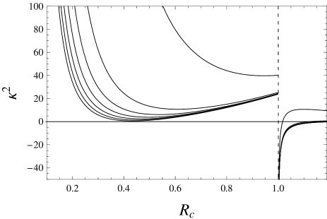
Figure 2: Behavior of quadratic epicyclic frequency for the model $n=1$, for $\tilde{M}_{1}/M_{p}=0.05,0.4,0.8,1.2,1.6,2,2.8$. For values larger than $\tilde{M}_{1}/M_{p}=2.8$ (bottom curve on the left and right sides),$\kappa^{2}$ is negative in the equatorial plane. For smaller values, $\kappa^{2}$ is greater and the gap of discontinuity at $R_{c}=a=1$ is smaller.

Figure 3 shows the behavior of the quadratic vertical frequency, also for the model $n=1$, and we note that it is a monotonically decreasing function, in the range $0\leq R_{c}\leq a$, with a minimum at $R_{c}=a$. In this case, to find the minimum value of $M_{p}$ (which we shall denote as $M_{p}^{**}$) for which $\nu^{2}(M_{p},R_{c})$ is positive, it is enough to solve the equation

$$\qquad\nu^{2}(M_{p}^{**},a)=0.$$

for the variable $M_{p}^{**}$. As in the previous case, we note that by increasing $M_{p}$, starting from $M_{p}^{**}$, the values of $\nu^{2}$ increase.

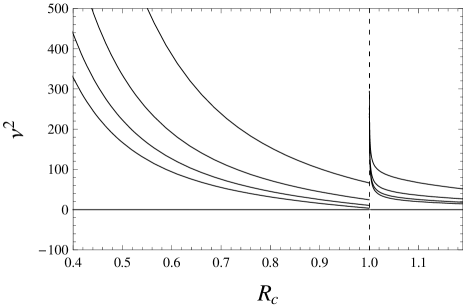
Figure 3: Behavior of quadratic vertical frequency for the model $n=1$, for $\tilde{M}_{1}/M_{p}=10^{-9},0.01,0.02,0.0485$. For values larger than $\tilde{M}_{1}/M_{p}=0.0485$ (bottom curve on the left side and top curve on the right side), $\nu^{2}$ is negative in the equatorial plane. For smaller values, $\nu^{2}$ is greater and the gap of discontinuity is smaller.

Another feature showed in figures 2 and 3 is that, for large values of $\tilde{M}_{1}/M_{p}$, the behavior of $\kappa^{2}$ and $\nu^{2}$ in the range $R_{c}>a$ is very different from the behavior in $0\leq R_{c}\leq a$. In general, we see that

$$\lim_{R_{c}\rightarrow a^{-}}\kappa^{2}\neq\lim_{R_{c}\rightarrow a^{+}}\kappa^{2}$$

(both are finite values), but the difference between these two limits is attenuated by decreasing the ratio $\tilde{M}_{1}/M_{p}$. We say that there is a gap of discontinuity at $R_{c}=a$. The same statements hold for $\nu^{2}$ and models with $n\geq 2$. It is clear that the gap disappear as $\tilde{M}_{1}/M_{p}\rightarrow 0$.

The behavior of epicyclic and vertical frequencies sketched above is the same for the other models $n=2,3,\ldots$, so that we can compute the maximum values of the rate $\tilde{M}_{n}/M_{p}$ leading to $\kappa^{2}>0$ or $\nu^{2}>0$. Such values are listed in Table 2, for the first ten members of the family (11). Since in all cases $\tilde{M}_{n}/M_{p}^{**}<\tilde{M}_{n}/M_{p}^{*}$, we can establish that $M_{p}^{**}$ is the parameter that determines the boundary between stability and instability in configurations characterized by gravitational potentials of the form (11).

$n$ $\tilde{M}_{n}/M_{p}^{*}$ $\tilde{M}_{n}/M_{p}^{**}$ 1 2.83102 0.04850 2 0.86297 0.02141 3 0.43398 0.01205 4 0.26554 0.00772 5 0.18068 0.00537

$n$ $\tilde{M}_{n}/M_{p}^{*}$ $\tilde{M}_{n}/M_{p}^{**}$ 6 0.13148 0.00395 7 0.10024 0.00303 8 0.07909 0.00240 9 0.06407 0.00194 10 0.05299 0.00161

Table 2: Ratios $\tilde{M}_{n}/M_{p}^{*}$ and $\tilde{M}_{n}/M_{p}^{**}$ for the first ten members of the family of configurations represented by (11). Here $M_{p}^{*}$ and $M_{p}^{**}$ are the minimum value of the central body’s mass such that $\kappa^{2}>0$ and $\nu^{2}>0$, respectively. In all cases $\tilde{M}_{n}/M_{p}^{*}>\tilde{M}_{n}/M_{p}^{**}$.

It is important to note that, in these models with fixed exterior radius $a$, the smaller the size of the $n$-th ring model, the larger is $M_{p}^{**}$. The reason is that, for higher members of the family (11), the ring’s mass concentration tends to be located near the outer edge and, therefore, away from the central monopole. Thus, it will be required increasingly central body mass to provide stability to the ring structure, as $n$ grows. This fact can be glimpsed through a comparison between tables 2 and 1, from which one might infer that there some kind of correlation between $\tilde{M}_{n}/M_{p}^{**}$ and the ring’s size of the family of models. In figure 4 we show this correlation by plotting the values of tables 2 and 1 and interpolating the corresponding points, for the first ten members of the family. Thus we can sketch a boundary between stability and instability of self-gravitating configurations under study. In figure 4, points located in the grey zone corresponds to parameters leading to stable configurations, while the points in the white region are associated to unstable configurations. We find that the points belonging to the sepparatrix of fig. 4 can be fitted by the relation

$$\tilde{M}_{n}/M_{p}^{**}\approx 0.065\exp\left(-4.67b_{n}/a\right).$$ (35)

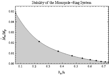
Figure 4: Correlation between the rate $\tilde{M}_{n}/M_{p}^{**}$ and $b_{n}/a$ according to the behavior of quadratic vertical frequency $\nu^{2}$ and quadratic epicyclic frequency $\kappa^{2}$. The interpolation line among points is a separatrix between a stability grey region, where $\nu^{2}>0$ and $\kappa^{2}>0$, and an instability white region, where $\nu^{2}<0$ (and $\kappa^{2}$ may be positive or negative). The points plotted here correspond to the first ten models, from left to right.

5 THE PHASE SPACE STRUCTURE

In this section, we shall make a description of three-dimensional motion through the study of phase space structure associated to orbits of test particles. We are principally interested in the influence of the mass ratio, in the regularity of three-dimensional bounded orbits. The influence of the size of the ring can be inferred from it, because in the models studied here, $b_{n}$ is automatically determined by $\tilde{M}_{n}$. This influence has already been analyzed in relation with the stability of equatorial circular orbits and now we extend such study to the case of more general orbits (remember that the motion restricted to the equatorial plane, which is completely integrable, can be exclusively classified as stable or unstable). In order to show how the nature of bounded motion is conditionated by the linear stability of the self-gravitating structures, we will use parameters close to the critical values we have defined previously (table 2). The influence of the quadrupolar deformation is considered in section 6.

We shall use cylindrical coordinates and plot $z=0$ surfaces of section corresponding to the equations of motion (12a)-(12b), for different values of the conserved quantities $E$ and $\ell$. It is worth to point out that we need to make explicit distinction between the orbits that cross the $z=0$ plane at $0\leq R\leq a$ and the ones that cross it only at $R>a$. The former are called disc-crossing orbits (DCO) and the latter we shall denote as non disc-crossing orbits (NDCO). The reason is that, for each of the above situations, the origin of irregular motion is different. For the case of DCO the discontinuity in the $z$-component of the gravitational field (equations (26a)-(26b)) can produce a fairly abrupt change in the curvature, leading to irregular motion (Saa 1999 ; Saa 2000 ; Hunter 2005 ; Ramos-Caro, López-Suspez & González 2008 ). Somehow, this is a problem analogous to the case of the chaotic behavior of Chua’s circuit (Matsumoto, Chua & Komuro 1985 ), which is described by an autonomous system of the type $\mathbf{\dot{x}}=f(\mathbf{x})$, where $f(\mathbf{x})$ is a piecewise function of class $\mathcal{C}^{0}$ (continuous but not differentiable). It is the first example where the existence of such class of function leads to the existence of a chaotic attractor in a dynamical system (Madan 1993 ).

In contrast, in the case of other three-dimensional orbits, chaotic motion is due to the existence of saddle points in the effective gravitational potential. Such saddle points, in the particular case of a potential as $\Phi^{*}_{n}$, will be located at equatorial plane, outside the disc (note that it is not possible to define saddle points inside the disc, due to the discontinuity in the potential’s $z$-derivative).

Equations (32) and (34) help us to investigate the existence of saddle points in the potential $\Phi^{*}_{n}$, through the evaluation of the quantity $\triangle=(\partial^{2}\Phi^{*}_{n}/\partial R^{2})(\partial^{2}\Phi^{*}_{n}/\partial z^{2})-(\partial^{2}\Phi^{*}_{n}/\partial R\partial z)^{2}$, which is negative when evaluated at saddle points. Since $\Phi^{*}_{n}$ is symmetric with respect to $z=0$, the term $\partial^{2}\Phi^{*}_{n}/\partial R\partial z$ vanishes at equatorial plane and the condition for existence of saddle points is reduced to $\triangle=\kappa^{2}\nu^{2}<0$. In the right side of figures 2 and 3 we can observe the behavior of $\kappa^{2}$ and $\nu^{2}<0$, respectively, and the product between them is showed in figure 5, for the case of model $m=1$. For different values of $\tilde{M}_{1}/M_{p}$ we note that there is a region of saddle points closed to the outer edge, even for the maximum value $0.0485$ leading to a stable configuration. When the ratio $\tilde{M}_{1}/M_{p}$ decreases and we have even more stable configurations, the range of saddle points decreases as well as the gap between the values of $\kappa^{2}\nu^{2}$ near the outer edge. This suggest that more and more stable configurations, produce less and less irregular orbits.

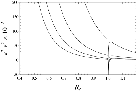
Figure 5: Behavior of the product $\kappa^{2}\nu^{2}$ for the values $\tilde{M}_{1}/M_{p}=10^{-9},0.01,0.02,0.0485$ (curves from top to bottom). For $\tilde{M}_{1}/M_{p}=0.0485$, the maximum value leading to a stable configuration, there is a small region of saddle points near to the outer edge (right side of the dashed line). This region becomes smaller as $\tilde{M}_{1}/M_{p}$ decreases.

In order to illustrate the above statements, we plot the surfaces of section corresponding to motion around the first two models, by choosing several values for the parameter $M_{p}$. We solve the equations of motion (12a)-(12b) by the Runge-Kutta 4th-method with variable time step and incorporating the Hénon algorithm (Hénon 1982 ), in the LCP (Laboratório de Computação Paralela) at IMECC. In the algorithm we take into account explicitly the discontinuity in the field force by implementing the set of equations (26a)-(27), as well as, the piecewise transformation (17)-(20). We choose initial conditions at $z=10^{-15}$, $V_{R}=0$ and several values for $R$ (the component $V_{z}$ is given by (14) and does not vanish). Orbits were integrated with a precision characterized by a relative error of $10^{-8}$ or less, in the energy conservation. Integrations were carried out on times of the order of $10^{5}$.

In figure 6 we have set $\tilde{M}_{1}/M_{p}=2.8$, which determine a radially stable configuration, but vertically unstable. There is a variety of central KAM curves and small resonant islands outside the disc zone as well as in the inner region. They alternate with two chaotic regions, one of them is due to DCO (the most prominent) and the other, more dense, is the result of two orbits near the saddle point ($R_{c}=1.014$ for this case). Here we have a situation where an unstable model admits a variety of irregular orbits.

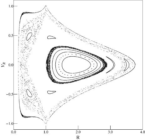
Figure 6: Surface of section for some orbits around the model $n=1$, with $\tilde{M}_{1}/M_{p}=2.8$. Such a rate determine an unstable situation, where $\kappa^{2}>0$ (marginally) but $\nu^{2}<0$. We find two chaotic regions: (i) A prominent zone due to DCO and (ii) a smaller zone corresponding to two orbits with initial conditions next to the saddle point. In this case, we have chosen $E=-0.3$ and $\ell=0.32$.

If we choose a more stable configuration, i.e. characterized by parameters near the sepparatrix of figure 4, we obtain surfaces of section as the shown in figure 7 where the chaotic region is restricted to the small central annulus enclosing the three KAM curves on the rigth. Note the presence of two chains of resonant islands enclosing the stochastic zone and other two small chains within it. In this case we find no chaotic motion associated to disc crossings, but only to exterior saddle points.

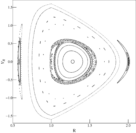
Figure 7: Surface of section corresponding to three-dimensional orbits around the model $n=1$, setting $\tilde{M}_{1}/M_{p}=0.0578$. The model represents an unstable situation (although very near to the separatrix of figure 4) and there are some chaotic orbits. The irregularity associated to these motions is due to the proximity to saddle point near to the disc edge. The orbits plotted have values $E=-6$ and $\ell=3.6$.

When we turn to the other side of the border, toward the region of stable configurations in figure 4, regularity is the most common feature of three dimensional orbits. Such is the case illustrated in figure 8, where we find only smooth KAM curves along the surface of section, even in the case of DCO orbits. In this case we can see a chain of 29 small resonant islands enclosing another chain of 3 central islands.

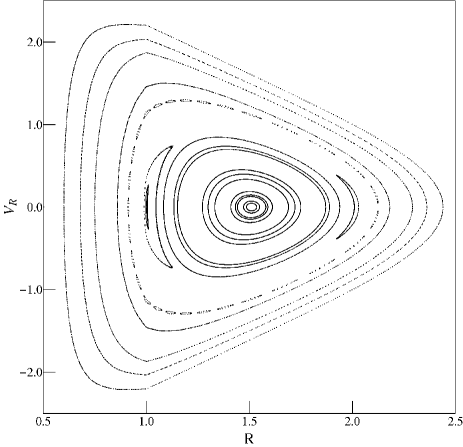
Figure 8: By maintaining the same values for $E$ and $\ell$ as in figure 7, but decreasing $\tilde{M}_{1}/M_{p}$ to $0.0485$, we find a situation when the $n=1$ model is stable (also very near to the separatrix of figure 4) and we note only regular orbits.

This transition from chaos to regularity, characterized by the apparition of increasingly number of islands when we pass from unstable to stable structures, can be seen in figures 9 and 10, which correspond to the model $n=2$. In the former there is a sequence of three prominent central islands, one of them enclosing a small chaotic region with a chain of 17 small resonant islands. In figure 10 the stochastic region is absent and we see only a dashed KAM curve enclosing three large islands.

It is clear that we expect a similar behavior for the remaining members of the infinite family: the increment of the mass of the spherical central body favors the existence of isolated islands in the phase space.

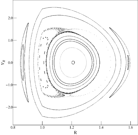
Figure 9: Surface of section corresponding to three-dimensional motion around the model $n=2$ with $\tilde{M}_{2}/M_{p}=0.0340$, for orbits with $E=-6$ and $\ell=4$. Since we are dealing with a configuration belonging to the unstable region of figure 4, there is a stochastic zone between a variety of regular KAM curves.

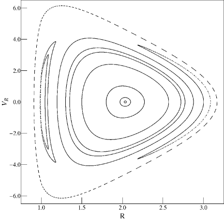
Figure 10: By maintaining the same values for $E$ and $\ell$ as in figure 9, and choosing $\tilde{M}_{2}/M_{p}=0.0214$, we obtain a situation when the $n=2$ model is stable and we note only regular orbits.

6 ADDITION OF QUADRUPOLAR TERM TO THE CENTRAL BODY

It is known that in the universe there exist many centers of attraction with a certain deviation from spherical symmetry, so we are interested in including a quadrupolar term in the description of the central object that makes up the structures studied above and examine the effects of deformation (preserving the axial symmetry). Now the gravitational potential of the structure is

$$\Phi_{n}^{(\beta)}=\tilde{\Phi}_{n}-\frac{GM_{p}}{\sqrt{R^{2}+z^{2}}}-\frac{\beta(2z^{2}-R^{2})}{2(R^{2}+z^{2})^{5/2}},$$ (36)

where $\beta$ is the quadrupolar moment that quantifies the oblate ($\beta<0$) or prolate ($\beta>0$) deformation of the central body. In general, it is related to the mass density $\rho(r,\theta)$ (axially symmetric) through the equation (Binney & Tremaine 2008 )

$$\beta=2\pi\int_{0}^{\infty}r^{4}dr\int_{0}^{\pi}d\theta\sin\theta P_{2}(\cos\theta)\rho(r,\theta),$$ (37)

where $r=\sqrt{R^{2}+z^{2}}$ and $\cos\theta=z/\sqrt{R^{2}+z^{2}}$ are the spherical coordinates.

The equations of motion for test particles around such configurations are the same (12a)-(12b) but replacing $\Phi_{n}$ by $\Phi_{n}^{(\beta)}$. Then, the relation for $\dot{V}_{R}$ inside the ring becomes

$$\dot{V}_{R} =\frac{\ell^{2}}{R^{3}}+\frac{3\beta}{\eta^{4}}-\frac{GM_{p}}{R^{2}}+\frac{R}{a\sqrt{a^{2}-R^{2}}}\left.\frac{\partial\tilde{\Phi}_{n}}{\partial\eta}\right|_{\eta=\sqrt{1-\frac{R^{2}}{a^{2}}}}^{\xi=0},$$ (38a)

while the relation for $\dot{V}_{z}$, in the inner, remains the same as in section 3. As a consequence, the relation that determines $\ell_{c}$, for inner circular orbits, changes to

$$\begin{split}\ell^{2}_{c}&=GM_{p}R_{c}-\frac{3\beta}{2R_{c}}-\frac{R_{c}^{4}}{a\sqrt{a^{2}-R_{c}^{2}}}\left.\frac{\partial\tilde{\Phi}_{n}}{\partial\eta}\right|^{\xi=0}_{\eta=\sqrt{1-R_{c}^{2}/a^{2}}}\\ &\qquad\qquad\qquad\qquad\qquad\qquad\qquad\qquad\mathrm{for}\>\>\>R_{c}<a,\end{split}$$ (39)

and, for outer circular orbits

$$\begin{split}\ell^{2}_{c}&=GM_{p}R_{c}-\frac{3\beta}{2R_{c}}+\frac{R_{c}^{4}}{a\sqrt{R_{c}^{2}-a^{2}}}\left.\frac{\partial\tilde{\Phi}_{n}}{\partial\xi}\right|^{\eta=0}_{\xi=\sqrt{R_{c}^{2}/a^{2}-1}}\\ &\qquad\qquad\qquad\qquad\qquad\qquad\qquad\qquad\mathrm{for}\>\>\>R_{c}>a.\end{split}$$ (40)

Therefore, the relations for the quadratic epicyclic frequency turns to

$$\begin{split}\kappa^{2}&=\frac{GM_{p}}{R_{c}^{3}}+\frac{6\beta}{R_{c}^{5}}+\frac{3R_{c}^{2}-4a^{2}}{a\left(a^{2}-R_{c}^{2}\right)^{3/2}}\left.\frac{\partial\tilde{\Phi}_{n}}{\partial\eta}\right|^{\xi=0}_{\eta=\sqrt{1-R_{c}^{2}/a^{2}}}\\ &+\frac{R_{c}^{2}}{a^{2}\left(a^{2}-R_{c}^{2}\right)}\left.\frac{\partial^{2}\tilde{\Phi}_{n}}{\partial\eta^{2}}\right|^{\xi=0}_{\eta=\sqrt{1-R_{c}^{2}/a^{2}}}\qquad\qquad\mathrm{for}\>\>\>R_{c}<a,\end{split}$$ (41)

and

$$\begin{split}\kappa^{2}&=\frac{GM_{p}}{R_{c}^{3}}+\frac{6\beta}{R_{c}^{5}}+\frac{3R_{c}^{2}-4a^{2}}{a\left(R_{c}^{2}-a^{2}\right)^{3/2}}\left.\frac{\partial\tilde{\Phi}_{n}}{\partial\xi}\right|^{\eta=0}_{\xi=\sqrt{R_{c}^{2}/a^{2}-1}}\\ &+\frac{R_{c}^{2}}{a^{2}\left(R_{c}^{2}-a^{2}\right)}\left.\frac{\partial^{2}\tilde{\Phi}_{n}}{\partial\xi^{2}}\right|^{\eta=0}_{\xi=\sqrt{R_{c}^{2}/a^{2}-1}}\qquad\qquad\mathrm{for}\>\>\>R_{c}>a,\end{split}$$ (42)

while for the vertical frequency we have now

$$\begin{split}\nu^{2}&=\frac{GM_{p}}{R_{c}^{3}}-\frac{9\beta}{2R_{c}^{5}}+\frac{R_{c}^{2}}{a\left(a^{2}-R_{c}^{2}\right)^{3/2}}\left.\frac{\partial\tilde{\Phi}_{n}}{\partial\eta}\right|^{\xi=0}_{\eta=\sqrt{1-R_{c}^{2}/a^{2}}}\\ &+\frac{1}{a^{2}-R_{c}^{2}}\left.\frac{\partial^{2}\tilde{\Phi}_{n}}{\partial\xi^{2}}\right|^{\xi=0}_{\eta=\sqrt{1-R_{c}^{2}/a^{2}}}\qquad\qquad\mathrm{for}\>\>\>R_{c}<a,\end{split}$$ (43)

and

$$\begin{split}\nu^{2}&=\frac{GM_{p}}{R_{c}^{3}}-\frac{9\beta}{2R_{c}^{5}}+\frac{R_{c}^{2}}{a\left(R_{c}^{2}-a^{2}\right)^{3/2}}\left.\frac{\partial\tilde{\Phi}_{n}}{\partial\xi}\right|^{\eta=0}_{\xi=\sqrt{R_{c}^{2}/a^{2}-1}}\\ &+\frac{1}{R_{c}^{2}-a^{2}}\left.\frac{\partial^{2}\tilde{\Phi}_{n}}{\partial\eta^{2}}\right|^{\eta=0}_{\xi=\sqrt{R_{c}^{2}/a^{2}-1}}\qquad\qquad\mathrm{for}\>\>\>R_{c}>a.\end{split}$$ (44)

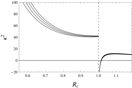
Figure 11: Behavior of $\kappa^{2}$ for $\tilde{M}_{1}/M_{p}=0.05$ and $\beta=0.1,0.2,0.3,0.4$ (curves from top to bottom). Maintaining the central monopole fixed, the epicyclic frequency grows as the quadrupolar moment decreases.

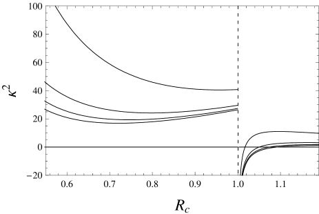
Figure 12: Behavior of $\kappa^{2}$ for $\beta=0.1$ and $\tilde{M}_{1}/M_{p}=0.05,0.15,0.25,0.35$ (curves from top to bottom). Maintaining the quadrupolar moment fixed, the epicyclic frequency grows as the central mass increases.

We note that the epicyclic frequency behaves in a very similar fashion as in the previous case of a spherically symmetric central body. This can be seen in figures 11 and 12. In the former we have chosen a certain fixed value for $M_{p}$ and plotted $\kappa^{2}$ for some positive values of quadrupolar moment (assuming prolate deformation), while in the latter we have fixed $\beta$ and plotted $\kappa^{2}$ for different values of $M_{p}$. These figures reveal that the quadratic epicyclic frequency is a positive concave function with a critical point in the range $0\leq R_{c}\leq a$. Needless to clarify that it is a monotonically decreasing function if we use negative values for $\beta$. Also, we have to point out that this quantity has the same behavior for the remaining models $n=2,3,...$ (the same statement holds for the vertical frequency).

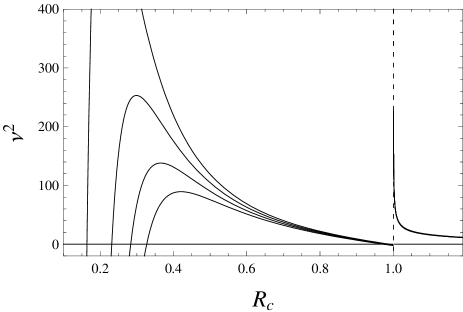
Figure 13: Behavior of $\nu^{2}$ for $\tilde{M}_{1}/M_{p}=0.05$ and $\beta=0.1,0.2,0.3,0.4$ (curves from top to bottom). Maintaining the central monopole fixed, the range where the quadratic vertical frequency is positive, grows as the quadrupolar moment decreases.

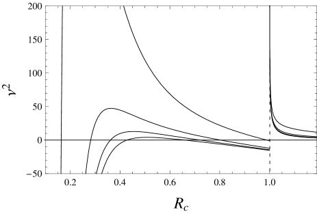
Figure 14: Behavior of $\nu^{2}$ for $\beta=0.1$ and $\tilde{M}_{1}/M_{p}=0.05,0.15,0.25,0.35$ (curves from top to bottom). Maintaining the quadrupolar moment fixed, the range where the quadratic vertical frequency is positive, grows as the central mass increases.

In contrast, the addition of a quadrupolar term introduces new features in the behavior of the quadratic vertical frequency. It can be observed from figures 13 and 14 that $\nu^{2}$ is now a negative concave function with a maximum in the range $0\leq R_{c}\leq a$, for positive values of quadrupolar moment (we have used the same values for the parameters as in figures 11 and 12). It is worth clarifying that, by using negative values for $\beta$, the quadratic vertical frequency becomes a monotonically decreasing function, as in the case of a spherically symmetric central body.

According to the above statements, the task to find the limiting values of $M_{p}$ and $\beta$, leading to stable configurations, is reduced to formulate the simultaneous equations

$$\nu^{2}(M_{p}^{{\dagger}},\beta^{{\dagger}},b_{n})=0,\qquad\nu^{2}(M_{p}^{{\dagger}},\beta^{{\dagger}},a)=0,$$

for the variables $M_{p}^{{\dagger}}$ and $\beta^{{\dagger}}$, i.e. the minimum value of the central body’s mass and the maximum value of the quadrupolar moment such that the quadratic vertical frequency (and evidently $\kappa^{2}$) is positive in the range between the cut-off radius and the outer radius. In table 3 we have listed the corresponding values of these quantities for the first ten members of the family. Consequently, we show the correlation between the logarithm of $\beta_{n}/\beta^{{\dagger}}$ and $\tilde{M}_{n}/M_{p}^{{\dagger}}$, plotting the separatrix between the stability and instability (fig. 15). Here, $\beta_{n}$ represents the quadrupolar moment of the $n$-th ring model and it is computed using equation (37). We find that the variables $x_{n}=\log_{10}(|\beta_{n}|/\beta)$ and $y_{n}=\log_{10}(|\tilde{M}_{n}|/M_{p}^{{\dagger}})$ can be fitted by the relation

$$y_{n}\approx-0.099x_{n}^{2}+0.345x_{n}-1.592,$$ (45)

providing an approximate expression for the separatrix of figure 15.

$n$ $\beta_{n}/\beta^{{\dagger}}$ $\tilde{M}_{n}/M_{p}^{{\dagger}}$ 1 -16.1076 0.04804 2 -0.55925 0.02024 3 -0.12408 0.01040 4 -0.04713 0.00602 5 -0.02301 0.00378

$n$ $\beta_{n}/\beta^{{\dagger}}$ $\tilde{M}_{n}/M_{p}^{{\dagger}}$ 6 -0.01300 0.00253 7 -0.00807 0.00177 8 -0.00537 0.00129 9 -0.00375 0.00097 10 -0.00273 0.00074

Table 3: Ratios $\tilde{M}_{n}/M_{p}^{{\dagger}}$ and $\beta_{n}/\beta^{{\dagger}}$ for the first ten members of the family given by (36). Here $M_{p}^{{\dagger}}$ and $\beta^{{\dagger}}$ represents the minimum value of mass and maximum value of quadrupolar moment such that the structure is linearly stable.

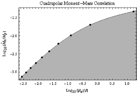
Figure 15: Correlation between the rate $\tilde{M}_{n}/M_{p}$ and $\beta_{n}/\beta$. The grey region represents the set of values leading to stable structures, while the white region corresponds to the stable ones.

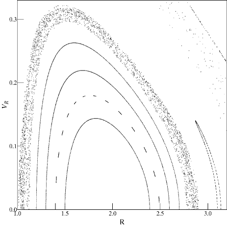
Figure 16: Detail of the central part of figure 6 corresponding to $n=1$, $\tilde{M}_{1}/M_{p}=2.8$ $E=-0.3$ and $\ell=0.32$. The inner stochastic region is generated by two orbits with initial conditions near the saddle point. The outer stochastic region is due to a DCO.

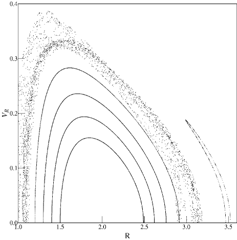
Figure 17: We have used the same parameters and initial conditions as in figure 16, but switching on the quadrupolar moment to $\beta=0.03$. The stochastic regions associated with this unstable configuration are distorted, with respect to the figure 16. The outer chaotic zone of DCO is absent, while the inner chaotic zone is more prominent.

As it was shown in Guéron & Letelier 2001 , for the case of monopole-quadrupole configurations, the chaoticity is induced by prolate (rather than oblate) deformation. In the case studied here, we have also a ring structure with oblate shape and one would expect two situations: (i) an “attenuation” in the chaoticity, for the case of a central body with prolate deformation; (ii) only regular motions, if the central body has also oblate shape.

The surfaces of section corresponding to structures located at stability region of figure 15 are not very different from those shown in plots 8 or 10. However, some differences appear when we deal with unstable configurations. For example, the outer stochastic region due to DCO, in figure 6, disappears when we turn on the quadrupolar moment, but the inner chaotic region is now most prominent and shifted slightly to the left (details are shown in figures 16 and 17).

7 Concluding Remarks

Simple models as the ones described by relations (8) and (10), provide us an useful tool to analyze and understand the dynamics of astrophysical objects that can be modeled as a spherical (or quasi-spherical) mass surrounded by a flat ring structure. One important and fundamental aspect in the dynamics is the stability against proper modes, if we consider in a first approximation that the ring structure is formed principally by particles moving in concentric circular orbits. It is known, in previous studies (Letelier 2007 ), that the structure of one ring standing alone has limited stability but, by adding a central monopole, it can improve. In this study we were able to verify such statement and find the set of values for the parameters leading to linearly stable configurations. Interestingly, we find monopole-ring configurations belonging to the stability region of figure 4, when dealing with parameters of the order of physical measurements performed in the solar system. For example, a structure with the dimensions of Saturn has $R_{min}/R_{max}\sim 0.1$ (ratio inner-outer radius) and $M_{ring}/M_{planet}\sim 10^{-8}$. Other example is a structure with $R_{min}/R_{max}\sim 0.4$ and $M_{ring}/M_{planet}\sim 10^{-11}$, similar to the parameters of Jupiter (Ellis et al. 2007 , Dougherty et al. 2009 ). We have to point out that a deeper stability analysis must include the effect of microstructure in the actual planetary rings (see for example Merlo & Benet 2007 ; Murray et al. 2008 ; Benet & Merlo 2009 ; Charnoz 2009 ; Charnoz et al. 2010 ).

On the other hand, there is a close connection between the stability of the configurations studied here, and the regularity of three dimensional orbits of test particles. We know that $\kappa^{2}$ and $\nu^{2}$ are piecewise functions with very different behavior when evaluated inside and outside the ring (figures 2 and 3). The piece corresponding to the inner region describes the linear stability of the ring, whereas the one corresponding to the outer zone is associated to the regularity or chaoticity in three dimensional motion (NDCO). We showed that each one of these pieces tend to be joined at the outer edge by increasing the central body mass (figure 5). This joining takes place in such a way that $\kappa^{2}$ and $\nu^{2}$ tend to be positive valued functions throughout the equatorial plane. This means that more and more stable configurations lead to a gradual decrease of chaoticity in three dimensional orbits, and the phase-space structure associated with them tends to be of the type of regular toroids.

It is worth to point out that the most relevant contribution to the stability in the configurations studied here, is provided by the mass of the central body. We can conclude that the increment of the monopolar term in the central body, rather than the decrease in the quadrupole moment, favors the existence of isolated islands in the phase space. The mass ratio and the size of the ring affects in the same way the stability of circular orbits (inside and outside the ring) and the regularity of three-dimensional motion (both DCO and NDCO). The fact that for DCO there exist a variety of regular islands throughout the phase-space, is relevant to confirm that the circular orbits supporting the ring structure are rather insensitive to small perturbations. Likewise, the above situation also holds for outer equatorial orbits and the associated three-dimensional motion (orbits without disc crossings) favoring the possible formation of new structures.

References

- (1) Arnold L., Schneider J., 2006, Direct Imaging of Exoplanets: Science & Techniques, Proceedings of the IAU Colloquium #200, 105, arXiv:astro-ph/0510594.
- (2) Arnold L.,Schneider J., 2004, A&A, 420, 1153, arXiv:astro-ph/0403330.
- (3) Barnes J. W., Fortney J. J., 2004, ApJ, 616 (2), 1193, arXiv:astro-ph/0409506.
- (4) Benet L., Merlo O., 2009, Celestial Mech. Dyn. Astr., 103 (3), 209, arXiv:0801.2030.
- (5) Benet L., Seligman T. H., 2000, Physics Letters A, 273 (5), 331, arXiv:nlin/0001018.
- (6) Binney J.,Tremaine S., 2008, Galactic Dynamics, 2nd Ed., Princeton University Press, Princeton, New Jersey.
- (7) Charnoz S., 2009, Icarus 201 (1), 191, arXiv:0901.0482.
- (8) Charnoz S., Salmon J., Crida A., 2010, Nature 465 (7299), 752.
- (9) Cuzzi J.N., Burns J.A., Charnoz S. et al., 2010, Science 327 (5972), 1470.
- (10) Dougherty M.K., Esposito L.W, Krimigis T., 2009, Saturn from Cassini-Huygens, Springer, New York.
- (11) Ellis D.M., Wessen R.R., Cuzzi J.N., 2007, Planetary Ring Systems, Springer-Praxis publishing, Berlin.
- (12) Goldreich P., Tremaine S., 1979, Nature 277, 97.
- (13) González G. A.,Reina J. I., 2006, MNRAS 371, 1873, arXiv:0806.4266.
- (14) Greenberg R.,Brahic A., 1984, Planetary rings, The University of Arizona Press, Tucson.
- (15) Guéron E., Letelier P. S. , 2001, Phys. Rev. E, 63, 035201, arXiv:astro-ph/0101164.
- (16) Hénon M., 1982, Physica D, 5, 412.
- (17) Holsapple K. A., 2001, Icarus, 154 (2), 432.
- (18) Hunter C., 2005, Ann. New York Acad. Sciences, 1045 (1), 120-138.
- (19) Hunter C.,Toomre A., 1969, ApJ 155, 747.
- (20) Jiang Z., 2000, MNRAS 319, 1067.
- (21) Jiang Z., Moss D., 2002, MNRAS 331, 117.
- (22) Jiang Z., Ossipkov L., 2007, MNRAS 379, 1133, arXiv:0708.3640.
- (23) Jones G. H. et al., 2008, Science (AAAS), 319 (5868), 1380.
- (24) Kalnajs A. J., 1972, ApJ 175, 63.
- (25) Kuzmin G. G., 1956, Astron. Zh., 33, 27.
- (26) Landau L.D., Lifshitz E.M. 1987, Pergamon Press, Oxford.
- (27) Lemos J. P. S.,Letelier P. S., 1994, Phys. Rev., 49, 5135.
- (28) Letelier P. S., 2003, PRD 68, 104002, arXiv:gr-qc/0309033.
- (29) Letelier P. S., 2007, MNRAS 381 (3), 1031, arXiv:0706.2802.
- (30) Longaretti P. Y., 1992, Planetary ring dynamics: from Boltzmann’s equation to celestial dynamics, Interrelations between physics and dynamics for minor bodies in the solar system, C. Froeschlé, Editions Frontières, Gif-sur-Yvette, 453.
- (31) Lora-Clavijo F. D., Ospina-Henao P. A., Pedraza, J. F., 2010, Phys. Rev. D82, 084005, arXiv:1009.1005.
- (32) Lord Rayleigh, 1916, Proc. R. Soc. London A93, 148.
- (33) Lynden-Bell D., 1962, MNRAS 123, 447.
- (34) Madan R. N., 1963, Chua’s circuit: a paradigm for chaos. Singapore: World Scientific.
- (35) Matsumoto T., Chua L., Komuro M.,1985, IEEE Transactions on Circuits and Systems 32 (8), 797.
- (36) Merlo O., Benet L., 2007, Celestial Mech. Dyn. Astr. 97, 49, arXiv:astro-ph/0609627.
- (37) Morgan T., Morgan L., 1969, Phys. Rev. 183, 1097.
- (38) Mestel L., 1963, MNRAS 126, 553.
- (39) Murray C.D., Chavez C., Beurle K. et al., 2005, Nature 437 (7063), 1326.
- (40) Murray C.D., Beurle K., Cooper N.J. et al., 2008, Nature 453 (7196), 739.
- (41) Ohta Y., Taruya A., Suto Y., 2009, ApJ, 690 (1), 1, arXiv:astro-ph/0611466.
- (42) Pedraza J. F.,Ramos-Caro J.,González G. A., 2008, MNRAS 390, 1587, arXiv:0806.4277.
- (43) Porco C.C., Baker E., Barbara J. et al., 2005, Science 307 (5713), 1226.
- (44) Ramos-Caro J., López-Suspez F., González G. A., 2008, MNRAS, 386, 440, arXiv:0806.4272.
- (45) Saa A., Venegeroles R., 1999, Phys. Lett. A, 259, 201, arXiv:gr-qc/9906028.
- (46) Saa A., 2000, Phys. Lett. A, 269, 204, arXiv:gr-qc/0003083.
- (47) Semerák O., Suková P., 2010, MNRAS, 404, 545.
- (48) Smith B. A., 1981, The Voyager imaging team, Science 212, 163.
- (49) Smith B. A., 1982, The Voyager imaging team, Science 215, 504.
- (50) Sicardy B., 2006, Dynamics of planetary rings, Dynamics of finite size celestial bodies and rings (A. Souchay Ed.), Springer-Verlag Berlin Heidelberg, Lect. Notes Phys., 682, 183.
- (51) Toomre A., 1963, ApJ 138, 385.
- (52) Toomre A., 1964, ApJ, 139, 1217.
- (53) Tresaco E., Ferrer S., 2010, Celest. Mech. Dyn. Astr, 107, 337.
- (54) Vogt D., Letelier P. S., 2009, MNRAS, 396 (3), 1487, arXiv:0906.0919.