Conformal Wasserstein Distances: Comparing Surfaces in Polynomial Time

Abstract.

We present a constructive approach to surface comparison realizable by a polynomial-time algorithm. We determine the “similarity” of two given surfaces by solving a mass-transportation problem between their conformal densities. This mass transportation problem differs from the standard case in that we require the solution to be invariant under global Möbius transformations. We present in detail the case where the surfaces to compare are disk-like; we also sketch how the approach can be generalized to other types of surfaces.

1. introduction

Alignment and comparison of surfaces (2-manifolds) play a central role in a wide range of scientific disciplines; they often constitute a crucial step in a variety of problems in medicine and biology.

Mathematically, the algorithmic problem of surface alignment amounts to defining a metric function $\mbox{\bf{d}}(\cdot,\cdot)$ in the space of Riemannian 2-manifolds with the following two properties: 1) for any two surfaces $\mathcal{M}$ and $\mathcal{N}$, $\mbox{\bf{d}}(\mathcal{M},\mathcal{N})=0$ implies that $\mathcal{M}$ and $\mathcal{N}$ are isometric, and 2) given a reasonably large number of reasonably well-distributed sample points on both surfaces, an accurate approximation to the distance $\mbox{\bf{d}}(\mathcal{M},\mathcal{N})$ can be calculated in a time that grows only polynomially in the sample set size. This second requirement is crucial to ensure that the algorithm can be used effectively in applications.

A prominent mathematical approach to define distances between surfaces that has been proposed for practical applications [10, 11] is the Gromov-Hausdorff (GH) distance; it considers the surfaces as special cases of metric spaces. To determine the GH distance between the metric spaces $X$ and $Y$, one examines all the isometric embeddings of $X$ and $Y$ into (other) metric spaces; although this distance possesses many attractive mathematical properties, it is inherently hard computationally. For instance, computing the $L_{p}$ version of the GH distance between two surfaces is equivalent to a non-convex quadratic programming problem, generally over the integers [9]. This problem is equivalent to integer quadratic assignment, and is thus NP-hard [13]. In [9], Memoli generalizes the GH distance of [10] by introducing a quadratic mass transportation scheme to be applied to metric spaces that are also equipped with a measure (mm spaces); the computation of this Gromov-Wasserstein (GW) distance for mm spaces is somewhat easier and more stable to implement than the original GH distance. The computation of the GW distance between two surfaces described in [9] utilizes a (continuous rather than integer) quadratic programming method; the functional to be minimized is generally not convex and optimization methods are likely to find local minima rather than the global minima that realizes the surfaces’ distance.

In this paper we propose a new surface alignment procedure, introducing the conformal Wasserstein distance. Our construction consists in “geometrically” aligning the surfaces, based on uniformization theory and optimal mass transportation. The uniformization theory serves as a “dimensionality reduction” tool, representing e.g. a disk-type surface by its conformal factor on the unit disk: the corresponding automorphism group (the disk-preserving Möbius group) has only three degrees of freedom and is therefore searchable in polynomial time. Next, the Kantorovich mass-transportation [3] is used to construct a linear functional the minimizer of which furnishes a metric; as is well-known [2, 4], this can solved by a linear program, and can thus be computed/approximated in polynomial time as-well.

As far as we know, prior to our work, no polynomial time algorithm was known to compute, either exactly or up to a good approximation, the GH distance or any other proposed intrinsic geometric distances between surfaces. Although [10] uses a mass transportation as well (albeit quadratic mass transportation), our approach is nevertheless different. We solve the “standard” (and thus linear) Kantorovich mass transportation problem, which is convex (even linear) and solvable via a linear programming method.

There exist earlier papers on aligning or comparing surfaces that use uniformization. In particular, the papers by Zeng et al. [Gu2008_a, Gu2008_b] which build upon the work of Gu and Yau [12], also use uniformization for surface alignment (albeit without defining a distance between surfaces). However, they use prescribed feature points (defined either by the user or by extra texture information) to calculate an interpolating harmonic map between the uniformization spaces, and then define the final correspondence as a composition of the uniformization maps and this harmonic interpolant. We use only intrinsic geometric information: we make use of the surfaces’ metric (inherited from its embedding in $\mathbb{R}^{3}$) and the induced conformal structure to define deviation from (local) isometry.

Optimal mass transportation has also been used before in aligning or comparing images. Following the seminal work by Rubner et al. [2], it is used extensively in the engineering literature to define interesting metric distances for images, interpreted as probability densities; in this context the metric is often called the ”Earth Mover’s Distance”.

Our paper is organized as follows: in Section 2 we briefly recall some facts about uniformization and optimal mass transportation that we shall use, at the same time introducing our notation. Section 3 contains the main results of this paper, constructing the conformal Wasserstein distance metric between disk-type surfaces, in several steps; we also indicate how the approach can be generalized to other surfaces. Section 4 briefly describes the discrete case.

2. Background and Notations

As described in the introduction, our framework makes use of two mathematical theories: uniformization theory, to represent the surfaces as measures defined on a canonical domain, and optimal mass transportation, to align the measures. In this section we recall some of their basic properties, and we introduce our notations.

2.1. Uniformization

By the celebrated uniformization theory for Riemann surfaces (see for example [7, 8]), any simply-connected Riemann surface is conformally equivalent to one of three canonical domains: the sphere, the complex plane, or the unit disk. Since every 2-manifold surface $\mathcal{M}$ equipped with a smooth Riemannian metric $g$ has an induced conformal structure and is thus a Riemann surface, uniformization applies to such surfaces. Therefore, every simply-connected surface with a Riemannian metric can be mapped conformally to one of the three canonical domains listed above. In this paper, we discuss 2D surfaces, equipped with a Riemannian metric tensor $g$ (possibly inherited from the standard 3D metric if the surface is embedded in $\mathbb{R}^{3}$) that have a finite total volume (i.e. area, since we are delaing with surfaces). For convenience, we shall normalize the metric so that the surface area equals 1. We shall discuss in detail the case where the surfaces $\mathcal{M}$ are topologically equivalent to disks. (We shall address in side remarks how the approach can be extended to the other cases.) For each such $\mathcal{M}$ there exists a conformal map $\phi:\mathcal{M}\rightarrow\mathcal{D}$, where $\mathcal{D}=\{z\ ;\ |z|<1\}$ is the open unit disk. (we assume that $\mathcal{M}$ does not include its boundary, if it has one). The map $\phi$ pushes $g$ to a metric on $\mathcal{D}$; denoting the coordinates in $\mathcal{D}$ by $z=x^{1}+\textbf{\footnotesize{i}}x^{2}$, we can write this metric as

$$\widetilde{g}=\phi_{*}g=\widetilde{\mu}(z)\,\delta_{ij}\,dx^{i}\otimes dx^{j},$$

where $\widetilde{\mu}(z)>0$, Einstein summation convention is used, and the subscript $*$ denotes the “push-forward” action. The function $\widetilde{\mu}$ can also be viewed as the density function of the measure $\mbox{\rm{vol}}_{\mathcal{M}}$ induced by the Riemann volume element: indeed, for (measurable) $A\subset\mathcal{M}$,

(2.1) $$\mbox{\rm{vol}}_{\mathcal{M}}(A)=\int_{\phi(A)}\widetilde{\mu}(z)\,dx^{1}\wedge dx^{2}.$$

It will be convenient to use the hyperbolic metric $(1-|z|^{2})^{-2}\delta_{ij}dx^{i}\otimes dx^{j}$ as the reference metric on the unit disk, rather than the standard Euclidean $\delta_{ij}dx^{i}\otimes dx^{j}$; note that the two are conformally equivalent (with conformal factor $(1-|z|^{2})^{-2}$). Instead of the density $\widetilde{\mu}(z)$, we shall therefore use the hyperbolic density function

(2.2) $$\mu^{H}(z):=(1-|z|^{2})^{2}\,\widetilde{\mu}(z)\,,$$

where the superscript $H$ stands for hyperbolic. We shall often drop this superscript: unless otherwise stated $\mu=\mu^{H}$, and $\nu=\nu^{H}$. This density function $\mu$ satisfies

$$\mbox{\rm{vol}}_{\mathcal{M}}(A)=\int_{\phi(A)}\mu(z)\,d\mbox{\rm{\footnotesize{vol}}}_{H}(z)\,,$$

where $d\mbox{\rm{\footnotesize{vol}}}_{H}(z)=(1-|z|^{2})^{-2}\,dx^{1}\wedge dx^{2}$. In what follows we shall use the symbol $\mu$ both for the function $\mu^{H}$ and as a shorthand for the absolutely continuous measure $\mbox{\rm{vol}}_{\mathcal{M}}$, and by extension for the surface $\mathcal{M}$ itself.

The conformal mappings of $\mathcal{D}$ to itself are the disk-preserving Möbius transformations $m\in M_{\mathcal{D}}$, a family with three real parameters, defined by

(2.3) $$m(z)=e^{\textbf{\footnotesize{i}}\theta}\frac{z-a}{1-\bar{a}z},\ a\in\mathcal{D},\ \theta\in[0,2\pi).$$

Since these Möbius transformations satisfy

(2.4) $$(1-|m(z)|^{2})^{-2}|m^{\prime}(z)|^{2}=(1-|z|^{2})^{-2}\,,$$

where $m^{\prime}$ stands for the derivatives of $m$, the pull-back of $\mu$ under a mapping $m\in M_{\mathcal{D}}$ takes on a particularly simple expression. Setting $w=m(z)$, with $w=y^{1}+\textbf{\footnotesize{i}}y^{2}$, and $\widetilde{g}(w)=\widetilde{\mu}(w)\delta_{ij}dy^{i}\otimes dy^{j}=\mu(w)(1-|w|^{2})^{-2}\delta_{ij}dy^{i}\otimes dy^{j}$, the definition

$$(m^{*}\widetilde{g})(z)_{kl}\,dx^{k}\otimes dx^{\ell}:=\mu(w)\,(1-|w|^{2})^{-2}\,\delta_{ij}\,dy^{i}\otimes dy^{j}$$

implies

$$(m^{*}\widetilde{g})_{k\ell}(z)\,dx^{k}\otimes dx^{\ell} =\mu(m(z))(1-|m(z)|^{2})^{-2}\,\delta_{ij}\,\frac{\partial y^{i}}{\partial x^{k}}\,\frac{\partial y^{j}}{\partial x^{\ell}}\,dx^{k}\otimes dx^{\ell}$$

$$=\mu(m(z))\,(1-|m(z)|^{2})^{-2}\,|m^{\prime}(z)|^{2}\,\delta_{k\ell}\,dx^{k}\otimes dx^{\ell}$$

$$=\mu(m(z))\,(1-|z|^{2})^{-2}\,\delta_{k\ell}\,dx^{k}\otimes dx^{\ell}.$$

In other words, $(m^{*}\widetilde{g})(z)_{kl}\,dx^{k}\otimes dx^{\ell}$ takes on the simple form $m^{*}\mu(z)\,(1-|z|^{2})^{-2}\,\delta_{kl}\,dx^{k}\otimes dx^{\ell}$, with

(2.5) $$m^{*}\mu(z)=\mu(m(z)).$$

Likewise, the push-forward, under a disk Möbius transform $m(z)=w$, of the (diagonal) Riemannian metric defined by the density function $\mu=\mu^{H}$, is again a diagonal metric, with (hyperbolic) density function $m_{*}\mu(w)=\left(m_{*}\mu\right)^{H}(w)$ given by

(2.6) $$m_{*}\mu(w)=\mu(m^{-1}(w)).$$

It follows that checking whether or not two surfaces $\mathcal{M}$ and $\mathcal{N}$ are isometric, or searching for (near-) isometries between $\mathcal{M}$ and $\mathcal{N}$, is greatly simplified by considering the conformal mappings from $\mathcal{M}$, $\mathcal{N}$ to $\mathcal{D}$: once the (hyperbolic) density functions $\mu$ and $\nu$ are known, it suffices to identify $m\in M_{\mathcal{D}}$ such that $\nu(m(z))$ and $\mu(z)$ coincide (or “nearly” coincide, in a sense to be made precise). This was exploited in [6] to construct fast algorithms to find corresponding points between two given surfaces. In the next section we provide a precise formalization of this idea using the notion of optimal mass transportation, described in the following subsection.

2.2. Optimal mass transportation

Optimal mass transportation was introduced by G. Monge [1], and L. Kantorovich [3]. It concerns the transformation of one mass distribution into another while minimizing a cost function that can be viewed as the amount of work required for the task. In the Kantorovich formulation, to which we shall stick in this paper, one considers two measure spaces $X,Y$ (each equipped with a $\sigma$-algebra), a probability measure on each, $\mu\in P(X)$, $\nu\in P(Y)$ (where $P(X),P(Y)$ are the respective spaces of all probability measures on $X$ and $Y$), and the space $\Pi(\mu,\nu)$ of probability measures $\pi$ on $X\times Y$ with marginals $\mu$ and $\nu$ (resp.), that is, for $A\subset X$, $B\subset Y$, $\pi(A\times Y)=\mu(A)$ and $\pi(X\times B)=\nu(B)$. The optimal mass transportation is the element of $\Pi(\mu,\nu)$ that minimizes $\int_{X\times Y}d(x,y)d\pi(x,y)$, where $d(x,y)$ is a cost function. (In general, one should consider an infimum rather than a minimum; in our case, $X$ and $Y$ are compact, $d(\cdot,\cdot)$ is continuous, and the infimum is achieved.) The corresponding minimum,

(2.7) $$T_{d}(\mu,\nu)=\mathop{\inf}_{\pi\in\Pi(\mu,\nu)}\int_{X\times Y}d(x,y)d\pi(x,y),$$

is the optimal mass transportation distance between $\mu$ and $\nu$, with respect to the cost function $d(x,y)$.

Intuitively, one can interpret this as follows: imagine being confronted with a pile of sand on the one hand (corresponding to $\mu$), and a hole in the ground on the other hand ($-\nu$), and assume that the volume of the sand pile equals exactly the volume of the hole (suitably normalized, $\mu,\nu$ are probability measures). You wish to fill the hole with the sand from the pile ($\pi\in\Pi(\mu,\nu)$), in a way that minimizes the amount of work (represented by $\int d(x,y)d\pi(x,y)$, where $d(\cdot,\cdot)$ can be thought of as a distance function).

In what follows, we shall apply this framework to the density functions $\mu$ and $\nu$ on the hyperbolic disk $\mathcal{D}$ obtained by conformal mappings from two surfaces $\mathcal{M}$, $\mathcal{N}$, as described in the previous subsection.

The Kantorovich transportation framework cannot be applied directly to the densities $\mu,\nu$. Indeed, the density $\mu$, characterizing the Riemannian metric on $\mathcal{D}$ obtained by pushing forward the metric on $\mathcal{M}$ via the uniformizing map $\phi:\mathcal{M}\rightarrow\mathcal{D}$, is not uniquely defined: another uniformizing map $\phi^{\prime}:\mathcal{M}\rightarrow\mathcal{D}$ may well produce a different $\mu^{\prime}$. Because the two representations are necessarily isometric ($\phi^{-1}\circ\phi^{\prime}$ maps $\mathcal{M}$ isometrically to itself), we must have $\mu^{\prime}(m(z))=\mu(z)$ for some $m\in M_{\mathcal{D}}$. (In fact, $m=\phi^{\prime}\circ\phi^{-1}$.) In a sense, the representation of (disk-type) surfaces $\mathcal{M}$ as measures over $\mathcal{D}$ should be considered “modulo” the disk Möbius transformations.

We thus need to address how to adapt the optimal transportation framework to factor out this Möbius transformation ambiguity. The next section starts by showing how this can be done.

3. The conformal Wasserstein framework: optimal volume transportation for surfaces

We want to measure distances between surfaces by using the Kantorovich transportation framework to measure the transportation between the metric densities on $\mathcal{D}$ obtained by uniformization applied to the surfaces. The main obstacle is that these metric densities are not uniquely defined; they are defined up to a Möbius transformation. In particular, if two densities $\mu$ and $\nu$ are related by $\nu=m_{*}\mu$ (i.e. $\mu(z)=\nu(m(z))$), where $m\in M_{\mathcal{D}}$, then we want our putative distance between $\mu$ and $\nu$ to be zero, since they describe isometric surfaces, and could have been obtained by different uniformization maps of the same surface. We thus want a distance metric between orbits of the group $M_{\mathcal{D}}$ acting on the conformal factors rather than a metric distance between the conformal factors themselves. If we choose a metric distance $d$ on $\mathcal{D}$ that is invariant under Möbius transformations, i.e. that it is a multiple of the hyperbolic distance on the disk, then a natural definition is as follows

(3.1) $$\mbox{\hausaD}(\mu,\nu)=\inf_{m\in M_{\mathcal{D}}}\left(\inf_{\pi\in\Pi(m_{*}\mu,\nu)}\,\int_{\mathcal{D}\times\mathcal{D}}d(z,w)\,d\pi(z,w)\,\right).$$

As shown in the Appendix, $\mbox{\hausaD}(\mu,\nu)$ is indeed a distance between disk-type surfaces; its computation can moreover be implemented in running times that grow only polynomially in the number $N$ of sample points used in the discretization of the surface (necessary to proceed to numerical computation). The optimization over $m$ in the definition of $\mbox{\hausaD}(\mu,\nu)$ always achieves its minimum in some $m$ (depending on $\mu$ and $\nu$ of course); denoting this special minimizing $m\in M_{\mathcal{D}}$ by $m_{\mu,\nu}$, we can rewrite $\mbox{\hausaD}(\mu,\nu)$ as the result of a single minimization (for details, see Appendix):

$$\mbox{\hausaD}(\mu,\nu) =\inf_{\pi\in\Pi([m_{\mu,\nu}]_{*}\mu,\nu)}\,\int_{\mathcal{D}\times\mathcal{D}}d(z,w)\,d\pi(z,w)$$

(3.2) $$=\inf_{\pi\in\Pi(\mu,\nu)}\,\int_{\mathcal{D}\times\mathcal{D}}d(m_{\mu,\nu}(z),w)\,d\pi(z,w)\,.$$

This is, however, purely formal; since the determination of $m_{\mu,\nu}$ involves the original double minimization of (3.1), a numerical implementation does require solving a mass-transportation functional for many $m\in M_{\mathcal{D}}$. In practice, this means that, despite its polynomial running time complexity, the numerical computation of $\mbox{\hausaD}(\mu,\nu)$ is too heavy for many applications, in which all pairwise distances must be computed for a collection of that may contain hundreds of surfaces [pnas]. This seems to lead to an impasse, since there exists no other distance metric on $\mathcal{D}$ that is conformally invariant, so that the natural “quotienting operation” over the group $M_{\mathcal{D}}$ can produce no other metric than $\mbox{\hausaD}(\cdot,\cdot)$.

However, $\mbox{\hausaD}(\mu,\nu)$, rewritten as in (3.2), suggests another way in which we can define an appropriate distance metric between orbits of the group $M_{\mathcal{D}}$ acting on the conformal factors. Note that (3.2) has exactly the same form as for a standard Kantorovich mass transportation scheme, except for the (crucial) difference that the cost function depends on $\mu$ and $\nu$. By retaining the idea of (Kantorovich) mass transportation, but allowing the use of cost functions $d(\cdot,\cdot)$ in the integrand that depend on $\mu$ and $\nu$ (without picking them necessarily of the form $d(m_{\mu,\nu}(z),w)$), we can construct other distance metrics $D$ on the conformal factors that are invariant under action of $M_{\mathcal{D}}$, i.e. for which $D(\mu,\nu)=D(m_{*}\mu,\nu)$ for all $m\in M_{\mathcal{D}}$. In addition, we can pick cost functions of this type ensuring that the distance between (or dissimilarity of) $\mu$ and $\nu$ exhibits some robustness with respect to deviations from global isometry. More precisely, we want the distance to be small for surfaces that are not isometric but nevertheless very close to isometric on parts of the surfaces; this can be achieved by picking a cost function $d^{R}_{\mu,\nu}(z,w)$ that depends on a comparison of the behavior of $\mu$ and $\nu$ on neighborhoods of $z$ and $w$, mapped by $m$ ranging over $M_{\mathcal{D}}$. This cost function, once incorporated in the Kantorovich mass transportation framework, will lead to a metric between disk-type surfaces (some generic conditions aside) based on solving a single mass transportation problem. The next subsection shows precisely how this is done. As is the case throughout the paper, we first give the full details of the construction for disk-like surfaces, and then indicate later how to generalize this to e.g. sphere-like surfaces. It is worthwhile to note that the “quotient approach” sketched above would not even have been applicable in a straightforward way to sphere-like surfaces, since they do not possess a metric invariant under all their Möbius transformations. As we shall explain at the end of this section, the same obstruction will not exist for the construction introduced in the next subsection.

3.1. Construction of $d^{R}_{\mu,\nu}(z,w)$

We construct $d^{R}_{\mu,\nu}(z,w)$ so that it indicates the extent to which a neighborhood of the point $z$ in $(\mathcal{D},\mu)$, the (conformal representation of the) first surface, is isometric with a neighborhood of the point $w$ in $(\mathcal{D},\nu)$, the (conformal representation of the) second surface. We will need to define two ingredients for this: the neighborhoods we will use, and how we shall characterize the (dis)similarity of two neighborhoods, equipped with different metrics.

We start with the neighborhoods.

For a fixed radius $R>0$, we define $\Omega_{z_{0},R}$ to be the hyperbolic geodesic disk of radius $R$ centered at $z_{0}$. The following gives an easy procedure to construct these disks. If $z_{0}=0$, then the hyperbolic geodesic disks centered at $z_{0}=0$ are also “standard” (i.e. Euclidean) disks centered at 0: $\Omega_{0,R}=\{z\,;\,|z|\leq r_{R}\}$, where $r_{R}=\mbox{tanh}(R)$. The hyperbolic disks around other centers are images of these central disks under Möbius transformations (= hyperbolic isometries): setting $m(z)=(z-z_{0})(1-z\bar{z_{0}})^{-1}$, we have

(3.3) $$\Omega_{z_{0},R}=m^{-1}(\Omega_{0,R})\,.$$

If $m^{\prime}$, $m^{\prime\prime}$ are two maps in $M_{\mathcal{D}}$ that both map $z_{0}$ to 0, then $m^{\prime\prime}\circ(m^{\prime})^{-1}$ simply rotates $\Omega_{0,R}$ around its center, over some angle $\theta$ determined by $m^{\prime}$ and $m^{\prime\prime}$. From this observation one easily checks that (3.3) holds for any $m\in M_{\mathcal{D}}$ that maps $z_{0}$ to $0$. In fact, we have the following more general

Lemma 3.1.

For arbitrary $z,w\in\mathcal{D}$ and any $R>0$, every disk preserving Möbius transformation $m\in M_{\mathcal{D}}$ that maps $z$ to $w$ (i.e. $w=m(z)$) also maps $\Omega_{z,R}$ to $\Omega_{w,R}$.

Next we define how to quantify the (dis)similarity of the pairs $\left(\Omega_{z_{0},R}\,,\,\mu\,\right)$ and $\left(\Omega_{w_{0},R}\,,\,\nu\,\right)$. Since (global) isometries are given by the elements of the disk-preserving Möbius group $M_{\mathcal{D}}$, we will test the extent to which the two patches are isometric by comparing $\left(\Omega_{w_{0},R}\,,\,\nu\,\right)$ with all the images of $\left(\Omega_{z_{0},R}\,,\,\mu\,\right)$ under Möbius transformations in $M_{\mathcal{D}}$ that take $z_{0}$ to $w_{0}$.

To carry out this comparison, we need a norm. Any metric $g_{ij}(z)dx^{i}\otimes dx^{j}$ induces an inner product on the space of 2-covariant tensors, as follows: if $\mathbf{a}(z)=a_{ij}(z)\,dx^{i}\otimes dx^{j}$ and $\mathbf{b}(z)=b_{ij}(z)\,dx^{i}\otimes dx^{j}$ are two 2-covariant tensors in our parameter space $\mathcal{D}$, then their inner product is defined by

(3.4) $$\langle\mathbf{a}(z),\mathbf{b}(z)\rangle=a_{ij}(z)\,b_{k\ell}(z)\,g^{ik}(z)\,g^{j\ell}(z)~{};$$

as always, this inner product defines a norm, $\|\mathbf{a}\|_{z}^{2}=a_{ij}(z)\,a_{k\ell}(z)\,g^{ik}(z)\,g^{j\ell}(z)$. Let us apply this to the computation of the norm of the difference between the local metric on one surface, $g_{ij}(z)=\mu(z)(1-|z|^{2})^{-2}\delta_{ij}$, and $h_{ij}(w)=\nu(w)(1-|w|^{2})^{-2}\delta_{ij}$, the pull-back metric from the other surface by a Möbius transformation $m$. Using (3.4), (2.5), and writing $\delta$, $g$, $h$, for the tensors with entries $\delta_{ij}$, $g_{ij}$, and $h_{ij}$, respectively, we have:

$$\|\mbox{\boldmath{$g$}}-m^{*}\mbox{\boldmath{$h$}}\|_{z}^{2} =\|\,\mu(z)(1-|z|^{2})^{-2}\mbox{\boldmath{$\delta$}}-\nu(m(z))(1-|z|^{2})^{-2}\mbox{\boldmath{$\delta$}}\,\|_{z}^{2}$$

$$=\Big{(}\mu(z)-\nu(m(z))\Big{)}^{2}(1-|z|^{2})^{-4}\,\delta_{ij}\,\delta_{k\ell}\,g^{ik}(z)\,g^{j\ell}(z)=\left(1-\frac{\nu(m(z))}{\mu(z)}\right)^{2}.$$

For every pair of $\mu,\,\nu$, we are now ready to define the distance function $d^{R}_{\mu,\nu}(\cdot,\cdot)$ on $\mathcal{D}$:

(3.5) $$d^{R}_{\mu,\nu}(z_{0},w_{0}):=\mathop{\mathop{\inf}_{m\in M_{\mathcal{D}}\,,}}_{m(z_{0})=w_{0}}\int_{\Omega_{z_{0},R}}\,|\,\mu(z)-(m^{*}\nu)(z)\,|\,d\mbox{\rm{\footnotesize{vol}}}_{H}(z),$$

where $d\mbox{\rm{\footnotesize{vol}}}_{H}(z)=(1-|z|^{2})^{-2}\,dx\wedge dy$ is the volume form for the hyperbolic disk. The integral in (3.5) can also be written in the following form, which makes its invariance more readily apparent:

(3.6) $$\int_{\Omega_{z_{0},R}}\left|\,1-\frac{\nu(m(z))}{\mu(z)}\right|\,d\mbox{\rm{\footnotesize{vol}}}_{\mathcal{M}}(z)=\int_{\Omega_{z_{0},R}}\|\mbox{\boldmath{$g$}}-m^{*}\mbox{\boldmath{$h$}}\|_{z}\,d\mbox{\rm{\footnotesize{vol}}}_{\mathcal{M}}(z),$$

where $d\mbox{\rm{\footnotesize{vol}}}_{\mathcal{M}}(z)=\mu(z)(1-|z|^{2})^{-2}\,dx^{1}\wedge dx^{2}=\sqrt{|g_{ij}|}\,dx^{1}\wedge dx^{2}$ is the volume form of the first surface $\mathcal{M}$.

The next Lemma shows that although the integration in (3.6) is carried out w.r.t. the volume of the first surface, this measure of distance is nevertheless symmetric:

Lemma 3.2.

If $m\in M_{\mathcal{D}}$ maps $z_{0}$ to $w_{0}$, $m(z_{0})=w_{0}$, then

$$\int_{\Omega_{z_{0},R}}\Big{|}\,\mu(z)-m^{*}\nu(z)\,\Big{|}\,d\mbox{\rm{\footnotesize{vol}}}_{H}(z)=\int_{\Omega_{w_{0},R}}\Big{|}\,m_{*}\mu(w)-\nu(w)\,\Big{|}\,d\mbox{\rm{\footnotesize{vol}}}_{H}(w).$$

Proof.

By the pull-back formula (2.5), we have

$$\int_{\Omega_{z_{0},R}}\Big{|}\,\mu(z)-m^{*}\nu(z)\,\Big{|}\,d\mbox{\rm{\footnotesize{vol}}}_{H}(z)=\int_{\Omega_{z_{0}}}\Big{|}\,\mu(z)-\nu(m(z))\,\Big{|}\,d\mbox{\rm{\footnotesize{vol}}}_{H}(z).$$

Performing the change of coordinates $z=m^{-1}(w)$ in the integral on the right hand side, we obtain

$$\int_{m(\Omega_{z_{0},R})}\,\Big{|}\,\mu(m^{-1}(w))-\nu(w)\Big{|}\,d\mbox{\rm{\footnotesize{vol}}}_{H}(w),$$

where we have used that $m^{-1}$ is an isometry and therefore preserves the volume element $d\mbox{\rm{\footnotesize{vol}}}_{H}(w)=(1-|w|^{2})^{-2}\,dy^{1}\wedge dy^{2}$. By Lemma 3.1, $\,m(\Omega_{z_{0},R})=\Omega_{w_{0},R}\,$; using the push-forward formula (2.6) then allows to conclude. ∎

Note that our point of view in defining our “distance” between $z$ and $w$ differs from the classical point of view in mass transportation: traditionally, $d(z,w)$ is some sort of physical distance between the points $z$ and $w$; in our case $d^{R}_{\mu,\nu}(z,w)$ measures the dissimilarity of (neighborhoods of) $z$ and $w$.

The next Theorem lists some important properties of $d^{R}_{\mu,\nu}$; its proof is given in the Appendix.

Theorem 3.3.

The distance function $d^{R}_{\mu,\nu}(z,w)$ satisfies the following properties

(1)	$~{}d^{R}_{m^{*}_{1}\mu,m^{*}_{2}\nu}(m^{-1}_{1}({z_{0}}),m^{-1}_{2}({w_{0}}))=d^{R}_{\mu,\nu}({z_{0}},{w_{0}})~{}$	Invariance under (well-defined)
		Möbius changes of coordinates
(2)	$~{}d^{R}_{\mu,\nu}({z_{0}},{w_{0}})=d^{R}_{\nu,\mu}({w_{0}},{z_{0}})~{}$	Symmetry
(3)	$~{}d^{R}_{\mu,\nu}({z_{0}},{w_{0}})\geq 0~{}$	Non-negativity
(4)	$\!\!\!\!\!\!d^{R}_{\mu,\nu}({z_{0}},{w_{0}})=0\,\Longrightarrow\,\Omega_{z_{0},R}$ in $(\mathcal{D},\mu)$ and $\Omega_{w_{0},R}$ in $(\mathcal{D},\nu)$ are isometric
(5)	$~{}d^{R}_{m^{*}\nu,\nu}(m^{-1}({z_{0}}),{z_{0}})=0~{}$	Reflexivity
(6)	$~{}d^{R}_{\mu_{1},\mu_{3}}(z_{1},z_{3})\leq d^{R}_{\mu_{1},\mu_{2}}(z_{1},z_{2})+d^{R}_{\mu_{2},\mu_{3}}(z_{2},z_{3})~{}$	Triangle inequality

In addition, the function $d^{R}_{\mu,\nu}:\mathcal{D}\times\mathcal{D}\,\rightarrow\,\mathbb{R}$ is continuous. To show this, we first look a little more closely at the 1-parameter family of disk Möbius transformations that map one pre-assigned point $z_{0}\in\mathcal{D}$ to another pre-assigned point $w_{0}\in\mathcal{D}$.

Definition 3.4.

For any pair of points $z_{0},\,w_{0}\in\mathcal{D}$, we denote by $M_{D,z_{0},w_{0}}$ the set of Möbius transformations that map $z_{0}$ to $w_{0}$.

This family of Möbius transformations is completely characterized by the following lemma:

Lemma 3.5.

For any $z_{0},w_{0}\in\mathcal{D}$, the set $M_{D,z_{0},w_{0}}$ constitutes a $1$-parameter family of disk Möbius transformations, parametrized continuously over $S^{1}$ (the unit circle). More precisely, every $m\in M_{D,z_{0},w_{0}}$ is of the form

(3.7) $$m(z)=\tau\,\frac{z-a}{1-\overline{a}z}~{},~{}~{}\mbox{ {\rm{with} }}~{}~{}a=a(z_{0},w_{0},\sigma):=\frac{z_{0}-w_{0}\,\overline{\sigma}}{1-\overline{z_{0}}\,w_{0}\,\overline{\sigma}}~{}~{}~{}\mbox{{\rm and }}~{}~{}\tau=\tau(z_{0},w_{0},\sigma):=\sigma\frac{1-\overline{z_{0}}\,w_{0}\,\overline{\sigma}}{1-z_{0}\,\overline{w_{0}}\,\sigma},$$

where $\sigma\in S_{1}:=\{z\in\mathbb{C}\,;\,|z|=1\}$ can be chosen freely.

Proof.

By (2.3), the disk Möbius transformations that map $z_{0}$ to $0$ all have the form

$$m_{\psi,z_{0}}(z)=e^{\textbf{\footnotesize{i}}\psi}\,\frac{z-z_{0}}{1-\overline{z_{0}}\,z}\,,~{}\mbox{ the inverse of which is }~{}~{}m_{\psi,z_{0}}^{-1}(w)=e^{-\textbf{\footnotesize{i}}\psi}\,\frac{w+e^{\textbf{\footnotesize{i}}\psi}z_{0}}{1+e^{-\textbf{\footnotesize{i}}\psi}\,\overline{z_{0}}w}~{},$$

where $\psi\in\mathbb{R}$ can be set arbitrarily. It follows that the elements of $M_{D,z_{0},w_{0}}$ are given by the family $m_{\gamma,w_{0}}^{-1}\circ m_{\psi,z_{0}}$, with $\psi,\,\gamma\in\mathbb{R}$. Working this out, one finds that these combinations of Möbius transformations take the form (3.7), with $\sigma=e^{\textbf{\footnotesize{i}}(\psi-\gamma)}$. ∎

We shall denote by $m_{z_{0},w_{0},\sigma}$ the special disk Möbius transformation defined by (3.7). In view of our interest in $d^{R}_{\mu,\nu}$, we also define the auxiliary function

$$\Phi : \mathcal{D}\times\mathcal{D}\times S_{1}\longrightarrow\mathbb{C}$$

$$(z_{0},w_{0},\sigma)\longmapsto\int_{\Omega_{z_{0},R}}\,|\,\mu(z)-\nu(m_{z_{0},w_{0},\sigma}(z))\,|\,d\mbox{\rm{\footnotesize{vol}}}_{H}(z)~{}.$$

This function has the following continuity properties, inherited from $\mu$ and $\nu$:

Lemma 3.6.

 
$\bullet$ For each fixed $(z_{0},w_{0})$, the function $\Phi(z_{0},w_{0},\cdot)$ is continuous on $S_{1}$.
$\bullet$ For each fixed $\sigma\in S_{1}$, $\Phi(\cdot,\cdot,\sigma)$ is continuous on $\mathcal{D}\times\mathcal{D}$. Moreover, the family $\Big{(}\Phi(\cdot,\cdot,\sigma)\Big{)}_{\sigma\in S_{1}}$ is equicontinuous.

Proof.

The proof of this Lemma is given in the Appendix. ∎

Note that since $S^{1}$ is compact, Lemma 3.6 implies that the infimum in the definition of $d^{R}_{\mu,\nu}$ can be replaced by a minimum:

$$d^{R}_{\mu,\nu}(z_{0},w_{0})=\mathop{\min}_{m(z_{0})=w_{0}}\,\int_{\Omega_{z_{0},R}}\,|\,\mu(z)-\nu(m(z))\,|\,d\mbox{\rm{\footnotesize{vol}}}_{H}(z)~{}.$$

We have now all the building blocks to prove

Theorem 3.7.

If $\mu$ and $\nu$ are continuous from $\mathcal{D}$ to $\mathbb{R}$, then $d^{R}_{\mu,\nu}(z,w)$ is a continuous function on $\mathcal{D}\times\mathcal{D}$.

Proof.

Pick an arbitrary point $(z_{0},w_{0})\in\mathcal{D}\times\mathcal{D}$, and pick $\varepsilon>0$ arbitrarily small.

By Lemma 3.6, there exists a $\delta>0$ such that, for $|z^{\prime}_{0}-z_{0}|<\delta$, $|w^{\prime}_{0}-w_{0}|<\delta$, we have

$$\left|\,\Phi(z_{0},w_{0},\sigma)-\Phi(z^{\prime}_{0},w^{\prime}_{0},\sigma)\,\right|\,\leq\,\varepsilon~{},$$

uniformly in $\sigma$. Pick now arbitrary $z^{\prime}_{0},w^{\prime}_{0}$ so that $|z_{0}-z^{\prime}_{0}|,|w_{0}-w^{\prime}_{0}|<\delta$.

Let $m_{z_{0},w_{0},\sigma}$, resp. $m_{z^{\prime}_{0},w^{\prime}_{0},\sigma^{\prime}}$, be the minimizing Möbius transform in the definition of $d_{\mu,\nu}^{R}(z_{0},w_{0})$, resp. $d_{\mu,\nu}^{R}(z^{\prime}_{0},w^{\prime}_{0})$, i.e.

$$d^{R}_{\mu,\nu}(z_{0},w_{0})=\Phi(z_{0},w_{0},\sigma)\ \ \textrm{and}\ \ d^{R}_{\mu,\nu}(z^{\prime}_{0},w^{\prime}_{0})=\Phi(z_{0},w_{0},\sigma^{\prime})~{}.$$

It then follows that

$$d^{R}_{\mu,\nu}(z_{0},w_{0}) =\min_{\tau}\Phi(z_{0},w_{0},\tau)\leq\Phi(z_{0},w_{0},\sigma^{\prime})$$

$$\leq\Phi(z^{\prime}_{0},w^{\prime}_{0},\sigma^{\prime})+|\Phi(z_{0},w_{0},\sigma^{\prime})-\Phi(z^{\prime}_{0},w^{\prime}_{0},\sigma^{\prime})|=d^{R}_{\mu,\nu}(z^{\prime}_{0},w^{\prime}_{0})+|\Phi(z_{0},w_{0},\sigma^{\prime})-\Phi(z^{\prime}_{0},w^{\prime}_{0},\sigma^{\prime})|$$

$$\leq d^{R}_{\mu,\nu}(z^{\prime}_{0},w^{\prime}_{0})+\mathop{\sup}_{\omega\in S_{1}}|\Phi(z_{0},w_{0},\omega)-\Phi(z^{\prime}_{0},w^{\prime}_{0},\omega)|\leq d^{R}_{\mu,\nu}(z^{\prime}_{0},w^{\prime}_{0})+\varepsilon~{}.$$

Likewise $d^{R}_{\mu,\nu}(z^{\prime}_{0},w^{\prime}_{0})\leq d^{R}_{\mu,\nu}(z_{0},w_{0})+\varepsilon$, so that $\left|d^{R}_{\mu,\nu}(z_{0},w_{0})-d^{R}_{\mu,\nu}(z^{\prime}_{0},w^{\prime}_{0})\right|<\varepsilon$. ∎

The function $d^{R}_{\mu,\nu}$ can be extended to a uniformly continuous function on the closed disk, by using the following lemma, proved in the Appendix.

Lemma 3.8.

Let $\left\{(z_{k},w_{k})\right\}_{k\geq 1}\subset\mathcal{D}\times\mathcal{D}$ be a sequence that converges, in the Euclidean norm, to some point in $(z^{\prime},w^{\prime})\in\overline{\mathcal{D}}\times\overline{\mathcal{D}}\setminus\mathcal{D}\times\mathcal{D}$, that is $|z_{k}-z^{\prime}|+|w_{k}-w^{\prime}|\rightarrow 0$, as $k\rightarrow\infty$. Then, $\lim_{k\rightarrow\infty}d^{R}_{\xi,\zeta}(z_{k},w_{k})$ exists and depends only on the limit point $(z^{\prime},w^{\prime})$.

3.2. Incorporating $d^{R}_{\mu,\nu}(z,w)$ into the transportation framework

The next step in constructing the distance operator between surfaces is to incorporate the distance $d^{R}_{\mu,\nu}(z,w)$ defined in the previous subsection into the (generalized) Kantorovich transportation model:

(3.8) $$T^{R}_{d}(\mu,\nu)=\inf_{\pi\in\Pi(\mu,\nu)}\int_{\mathcal{D}\times\mathcal{D}}d^{R}_{\mu,\nu}(z,w)d\pi(z,w).$$

The main result is that this procedure (under some extra conditions) furnishes a metric between (disk-type) surfaces.

Theorem 3.9.

There exists $\pi^{*}\in\Pi(\mu,\nu)$ such that

$$\int_{\mathcal{D}\times\mathcal{D}}d^{R}_{\mu,\nu}(z,w)d\pi^{*}(z,w)=\inf_{\pi\in\Pi(\mu,\nu)}\int_{\mathcal{D}\times\mathcal{D}}d^{R}_{\mu,\nu}(z,w)d\pi(z,w).$$

Proof.

With a slight abuse of notation, we denote by $\mu$ the probability measure on $\mathcal{D}$ that is absolutely continuous with respect to the hyperbolic measure on $\mathcal{D}$, with density function equal to the continous function $\mu$ on $\mathcal{D}$. (See subsection 2.1.) We now define a probability measure $\overline{\mu}$ on $\overline{\mathcal{D}}\,$ by setting $\overline{\mu}(A)=\mu(A\cap\mathcal{D})$, for arbitrary Borel sets $A\subset\overline{\mathcal{D}}\,$; $\overline{\nu}$ is defined analogously. By the Riesz-Markov theorem, the space of probability measures $\mathcal{P}(\overline{\mathcal{D}}\times\overline{\mathcal{D}})$ can be viewed as a (closed) subset of the unit ball in $C(\overline{\mathcal{D}}\times\overline{\mathcal{D}})^{*}$. As such, both $\mathcal{P}(\overline{\mathcal{D}}\times\overline{\mathcal{D}})$ and its closed subset $\Pi(\overline{\mu},\overline{\nu})$ are weak$*$-compact, by the Banach-Alaoglu theorem. Note that for each $\overline{\pi}\in\Pi(\overline{\mu},\overline{\nu})$, we have

$$\overline{\pi}(\mathcal{D}\times\mathcal{D})\geq\overline{\pi}(\overline{\mathcal{D}}\times\overline{\mathcal{D}})-\left(\overline{\pi}(\overline{\mathcal{D}}\times[\overline{\mathcal{D}}\setminus\mathcal{D}])+\overline{\pi}([\overline{\mathcal{D}}\setminus\mathcal{D}]\times\overline{\mathcal{D}})\right)\,=\,1-\overline{\nu}(\overline{\mathcal{D}}\setminus\mathcal{D})-\overline{\mu}(\overline{\mathcal{D}}\setminus\mathcal{D})\,=\,1\,,$$

and thus $\overline{\pi}(\mathcal{D}\times\mathcal{D})=1$; the restriction $\pi$ of each such $\overline{\pi}$ to the Borel sets contained in $\mathcal{D}\times\mathcal{D}$ is thus a probability measure on $\mathcal{D}\times\mathcal{D}$.
Since (the extension to $\overline{\mathcal{D}}\times\overline{\mathcal{D}}$ of) $d_{\mu,\nu}(\cdot,\cdot)$ is an element of $C(\overline{\mathcal{D}}\times\overline{\mathcal{D}})$ by Lemma 3.8, it follows that the evaluation $\,\overline{\pi}\mapsto\overline{\pi}(d_{\mu,\nu})\,=\,\int_{\overline{\mathcal{D}}\times\overline{\mathcal{D}}}\,d_{\mu,\nu}(z,w)\,d\overline{\pi}(z,w)\,=\,\int_{\mathcal{D}\times\mathcal{D}}\,d_{\mu,\nu}(z,w)\,d{\pi}(z,w)\,$ is weak$*$-continuous on the weak$*$-compact set $\Pi(\overline{\mu},\overline{\nu})$; it thus achieves its infimum in an element $\overline{\pi^{*}}$ of that set. As observed above, $\pi^{*}$, the restriction of $\overline{\pi^{*}}$ to the Borel sets contained in $\mathcal{D}\times\mathcal{D}$, is a probability measure on $\mathcal{D}\times\mathcal{D}$, and an element of $\Pi({\mu},{\nu})$; this is the desired minimizer.

∎

Under rather mild conditions, the “standard” Kantorovich transportation (2.7) on a metric spaces $(X,d)$ defines a metric on the space of probability measures on $X$ . We will prove that our generalization defines a distance metric as well. More precisely, we shall prove first that

$$\mbox{\bf{d}}^{R}(\mathcal{M},\mathcal{N})=T^{R}_{d}(\mu,\nu)$$

defines a semi-metric in the set of all disk-type surfaces. We shall restrict ourselves to surfaces that are sufficiently smooth to allow uniformization, so that they can be globally and conformally parametrized over the hyperbolic disk. Under some extra assumptions, we will prove that $\mbox{\bf{d}}^{R}$ is a metric, in the sense that $\mbox{\bf{d}}^{R}(\mathcal{M},\mathcal{N})=0$ implies that $\mathcal{M}$ and $\mathcal{N}$ are isometric.

For the semi-metric part we will again adapt a proof given in [4] to our framework. In particular, we shall make use of the following “gluing lemma”:

Lemma 3.10.

Let $\mu_{1},\mu_{2},\mu_{3}$ be three probability measures on $\mathcal{D}$, and let $\pi_{12}\in\Pi(\mu_{1},\mu_{2})$, $\pi_{23}\in\Pi(\mu_{2},\mu_{3})$ be two transportation plans. Then there exists a probability measure $\pi$ on $\mathcal{D}\times\mathcal{D}\times\mathcal{D}$ that has $\pi_{12},\pi_{23}$ as marginals, that is $\int_{z_{3}\in\mathcal{D}}d\pi(z_{1},z_{2},z_{3})=d\pi_{12}(z_{1},z_{2})$, and $\int_{z_{1}\in\mathcal{D}}d\pi(z_{1},z_{2},z_{3})=d\pi_{23}(z_{2},z_{3})$.

This lemma will be used in the proof of the following:

Theorem 3.11.

For two disk-type surfaces $\mathcal{M}=(\mathcal{D},\mu)$, $\mathcal{N}=(\mathcal{D},\nu)$, let $\mbox{\bf{d}}^{R}(\mathcal{M},\mathcal{N})$ be defined by

$$\mbox{\bf{d}}^{R}(\mathcal{M},\mathcal{N})=T^{R}_{d}(\mu,\nu).$$

Then $\mbox{\bf{d}}^{R}$ defines a semi-metric on the space of disk-type surfaces.

Proof.

The symmetry of $d^{R}_{\mu,\nu}$ implies symmetry for $T^{R}_{d}$, by the following argument:

$$T^{R}_{d}(\mu,\nu) =\mathop{\inf}_{\pi\in\Pi(\mu,\nu)}\int_{\mathcal{D}\times\mathcal{D}}d^{R}_{\mu,\nu}(z,w)d\pi(z,w)=\mathop{\inf}_{\pi\in\Pi(\mu,\nu)}\int_{\mathcal{D}\times\mathcal{D}}d^{R}_{\nu,\mu}(w,z)d\pi(z,w)$$

$$=\mathop{\inf}_{\pi\in\Pi(\mu,\nu)}\int_{\mathcal{D}\times\mathcal{D}}d^{R}_{\nu,\mu}(w,z)d\widetilde{\pi}(w,z),~{}~{}~{}~{}~{}~{}~{}\mbox{ where we have set }~{}\widetilde{\pi}(w,z)=\pi(z,w)$$

$$=T^{R}_{d}(\nu,\mu)~{}.~{}~{}~{}~{}~{}~{}~{}~{}~{}(\mbox{ use that }\pi\in\Pi(\mu,\nu)\Leftrightarrow\widetilde{\pi}\in\Pi(\nu,\mu))$$

The non-negativity of $d^{R}_{\mu,\nu}(\cdot,\cdot)$ automatically implies $T^{R}_{d}(\mu,\nu)\geq 0$.

Next we show that, for any Möbius transformation $m$, $T^{R}_{d}(\mu,m_{*}\mu)=0$. To see this, pick the transportation plan $\pi\in\Pi(\mu,m_{*}\mu)$ defined by

$$\int_{\mathcal{D}\times\mathcal{D}}f(z,w)d\pi(z,w)=\int_{\mathcal{D}}f(z,m(z))\mu(z)\,d\mbox{\rm{\footnotesize{vol}}}_{H}(z).$$

On the one hand $\pi\in\Pi(\mu,m_{*}\mu)$, since

$$\int_{A\times\mathcal{D}}d\pi(z,w)=\int_{A}\mu(z)d\mbox{\rm{\footnotesize{vol}}}_{H}(z),$$

and

$$\int_{\mathcal{D}\times B}d\pi(z,w) =\int_{\mathcal{D}\times\mathcal{D}}\chi_{B}(w)d\pi(z,w)$$

$$=\int_{\mathcal{D}}\chi_{B}(m(z))\mu(z)d\mbox{\rm{\footnotesize{vol}}}_{H}(z)=\int_{\mathcal{D}}\chi_{B}(w)\mu_{*}(w)d\mbox{\rm{\footnotesize{vol}}}_{H}(w),$$

where we used the change of variables $w=m(z)$ in the last step. Furthermore, $\pi(z,w)$ is concentrated on the graph of $m$, i.e. on $\left\{(z,m(z))\ ;\ z\in\mathcal{D}\right\}\subset\mathcal{D}\times\mathcal{D}$. Since $d^{R}_{\mu,m_{*}\mu}(z,m(z))=0$ for all $z\in\mathcal{D}$ we obtain therefore $T_{d}(\mu,m_{*}\mu)\leq\int_{\mathcal{D}\times\mathcal{D}}d^{R}_{\mu,m_{*}\mu}(z,w)d\pi(z,w)=0$.

Finally, we prove the triangle inequality $T^{R}_{d}(\mu_{1},\mu_{3})\leq T^{R}_{d}(\mu_{1},\mu_{2})+T^{R}_{d}(\mu_{2},\mu_{3})$ . To this end we follow the argument in the proof given in [4] (page 208). This is where we invoke the gluing Lemma stated above.

We start by picking arbitrary transportation plans $\pi_{12}\in\Pi(\mu_{1},\mu_{2})$ and $\pi_{23}\in\Pi(\mu_{2},\mu_{3})$. By Lemma 3.10 there exists a probability measure $\pi$ on $\mathcal{D}\times\mathcal{D}\times\mathcal{D}$ with marginals $\pi_{12}$ and $\pi_{23}$. Denote by $\pi_{13}$ its third marginal, that is

$$\int_{z_{2}\in\mathcal{D}}d\pi(z_{1},z_{2},z_{3})=d\pi_{13}(z_{1},z_{3}).$$

Then

$$T^{R}_{d}(\mu_{1},\mu_{3}) \leq\int_{\mathcal{D}\times\mathcal{D}}d^{R}_{\mu_{1},\mu_{3}}(z_{1},z_{3})d\pi_{13}(z_{1},z_{3})=\int_{\mathcal{D}\times\mathcal{D}\times\mathcal{D}}d^{R}_{\mu_{1},\mu_{3}}(z_{1},z_{3})d\pi(z_{1},z_{2},z_{3})$$

$$\leq\int_{\mathcal{D}\times\mathcal{D}\times\mathcal{D}}\Big{(}d^{R}_{\mu_{1},\mu_{2}}(z_{1},z_{2})+d^{R}_{\mu_{2},\mu_{3}}(z_{2},z_{3})\Big{)}d\pi(z_{1},z_{2},z_{3})$$

$$\leq\int_{\mathcal{D}\times\mathcal{D}\times\mathcal{D}}d^{R}_{\mu_{1},\mu_{2}}(z_{1},z_{2})d\pi(z_{1},z_{2},z_{3})+\int_{\mathcal{D}\times\mathcal{D}\times\mathcal{D}}d^{R}_{\mu_{2},\mu_{3}}(z_{2},z_{3})d\pi(z_{1},z_{2},z_{3})$$

$$\leq\int_{\mathcal{D}\times\mathcal{D}}d^{R}_{\mu_{1},\mu_{2}}(z_{1},z_{2})d\pi_{12}(z_{1},z_{2})+\int_{\mathcal{D}\times\mathcal{D}}d^{R}_{\mu_{2},\mu_{3}}(z_{2},z_{3})d\pi_{23}(z_{2},z_{3}),$$

where we used the triangle-inequality for $d^{R}_{\mu,\nu}$ listed in (Theorem 3.3). Since we can choose $\pi_{12}$ and $\pi_{23}$ to achieve arbitrary close values to the infimum in eq. (3.8) the triangle inequality follows. ∎

To qualify as a metric rather than a semi-metric, $\mbox{\bf{d}}^{R}$ (or $T^{R}_{d}$) should be able to distinguish from each other any two surfaces (or measures) that are not “identical”, that is isometric. To prove that they can do so, we need an extra assumption: we shall require that the surfaces we consider have no self-isometries. More precisely, we require that each surface $\mathcal{M}$ that we consider satisfies the following definition:

Definition 3.12.

A disk-type surface $\mathcal{M}$ is said to be singly $\varrho\mbox{-}_{\mbox{\tiny{H}}}\mbox{fittable}$ (where $\varrho\in\mathbb{R},$ $\varrho>0$) if, for all $R>\varrho$, all $z_{0}\in\mathcal{D}$, and all conformal factors obtained in uniformizations of the disk $\mathcal{M}\,$ there is no other Möbius transformation $m$ other than the identity for which

$$\int_{\Omega_{z_{0},R}}\,|\mu(z)-\mu(m(z))|\,d\mbox{\rm{\footnotesize{vol}}}_{H}(z)=0\,.$$

Remark 3.13.

This definition can also be read as follows: $\mathcal{M}$ is singly $\varrho\mbox{-}_{\mbox{\tiny{H}}}\mbox{fittable}$ if and only if, for all $R>\varrho$, any two conformal factors $\mu_{1}$ and $\mu_{2}$ for $\mathcal{M}$ satisfy:

1. For all $z\in\mathcal{D}$ there exists a unique minimum to the function $w\mapsto d^{R}_{\mu_{1},\mu_{2}}(z,w)$.

2. For all pairs $(z,w)\in\mathcal{D}\times\mathcal{D}$ that achieve this minimum there exists a unique Möbius transformation for which the integral in (3.5) vanishes (with $\mu_{1}$ in the role of $\mu$, and $\mu_{2}$ in that of $\nu$).

Note that in order to ensure that the conditions in the definition hold for all conformal factors, it is sufficient to require that it holds for the conformal factor associated to just one uniformization.

Essentially, this definition requires that, from some sufficiently large (hyperbolic) scale onwards, there are no isometric pieces within $(\mathcal{D},\mu)$ (or $(\mathcal{D},\nu)$).

We are ready to prove the last remaining part of the main result of this subsection. We start with a lemma.

Lemma 3.14.

Let $\pi\in\Pi(\mu,\nu)$ be such that $\int_{\mathcal{D}\times\mathcal{D}}\,d^{R}_{\mu,\nu}(z,w)\,d\pi(z,w)=0$. Then, for all $z_{0}\in\mathcal{D}$ and $\delta>0$, there exists at least one point $z\in\Omega_{z_{0},\delta}$ such that $d^{R}_{\mu,\nu}(z,w)=0$ for some $w\in\mathcal{D}$.

Proof.

By contradiction: assume that there exists a disk $\Omega_{z_{0},\delta}$ such that $d^{R}_{\mu,\nu}(z,w)>0$ for all $z\in\Omega_{z_{0},\delta}$ and all $w\in\mathcal{D}$. Since

$$\int_{\Omega(z_{0},\delta)\times\mathcal{D}}\,d\pi(z,w)=\int_{\Omega(z_{0},\delta)}\mu(z)\,d\mbox{\rm{\footnotesize{vol}}}_{H}(z)>0~{},$$

the set $\Omega(z_{0},\delta)\times\mathcal{D}$ contains some of the support of $\pi$. It follows that

$$\int_{\Omega(z_{0},\delta)\times\mathcal{D}}d^{R}_{\mu,\nu}(z,w)\,d\pi(z,w)>0~{},$$

which contradicts

$$\int_{\Omega(z_{0},\delta)\times\mathcal{D}}d^{R}_{\mu,\nu}(z,w)d\pi(z,w)\leq\int_{\mathcal{D}\times\mathcal{D}}d^{R}_{\mu,\nu}(z,w)d\pi(z,w)=0~{}.$$

∎

Theorem 3.15.

Suppose that $\mathcal{M}$ and $\mathcal{N}$ are two surfaces that are singly $\varrho\mbox{-}_{\mbox{\tiny{H}}}$fittable. If $\mbox{\bf{d}}^{R}(\mathcal{M},\mathcal{N})=0$ for some $R>\varrho$, then there exists a Möbius transformation $m\in M_{\mathcal{D}}$ that is a global isometry between $\mathcal{M}=(\mathcal{D},\mu)$ and $\mathcal{N}=(\mathcal{D},\nu)$ (where $\mu$ and $\nu$ are conformal factors of $\mathcal{M}$ and $\mathcal{N}$, respectively).

Proof.

When $\mbox{\bf{d}}^{R}(\mathcal{M},\mathcal{N})=0$, there exists (see [4]) $\pi\in\Pi(\mu,\nu)$ such that

$$\int_{\mathcal{D}\times\mathcal{D}}d^{R}_{\mu,\nu}(z,w)d\pi(z,w)=0.$$

Next, pick an arbitrary point $z_{0}\in\mathcal{D}$ such that, for some $w_{0}\in\mathcal{D}$, we have $d^{R}_{\mu,\nu}(z_{0},w_{0})=0$. (The existence of such a pair is guaranteed by Lemma 3.14.) This implies that there exists a unique Möbius transformation $m_{0}\in M_{\mathcal{D}}$ that takes $z_{0}$ to $w_{0}$ and that satisfies $\nu(m_{0}(z))=\mu(z)$ for all $z\in\Omega_{z_{0},R}$. We define

$$\rho^{*}=\sup\{\rho\,;\,d^{\rho}_{\mu,\nu}(z_{0},w_{0})=0\};$$

clearly $\rho^{*}\geq R$. The theorem will be proved if we show that $\rho^{*}=\infty$. We shall do this by contradiction.

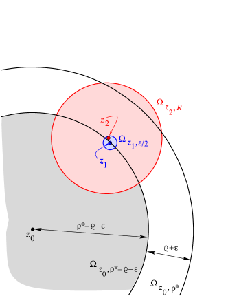
Figure 1. Illustration of the proof of Theorem 3.15

Assume $\rho^{*}<\infty$. Consider $\Omega_{z_{0},\rho^{*}}$, the hyperbolic disk around $z_{0}$ of radius $\rho^{*}$. (See Figure 1 for illustration.) Set $\varepsilon=(R-\varrho)/2$, and consider the points on the hyperbolic circle $C=\partial\Omega_{z_{0},\rho^{*}-\varrho-\varepsilon}$. For every $z_{1}\in C$, consider the hyperbolic disk $\Omega_{z_{1},\varepsilon/2}$; by Lemma 3.14 there exists a point $z_{2}$ in this disk and a corresponding point $w_{2}\in\mathcal{D}$ such that $d^{R}_{\mu,\nu}(z_{2},w_{2})=0$, i.e. such that

$$\int_{\Omega_{z_{2},R}}\,|\mu(z)-m^{\prime*}\nu(z)|\,d\mbox{\rm{\footnotesize{vol}}}_{H}(z)\,=\,0~{}$$

for some Möbius transformation $m^{\prime}$ that maps $z_{2}$ to $w_{2}$; in particular, we have that

(3.9) $$\mu(z)=\nu(m^{\prime}(z))~{}~{}\mbox{ for all }~{}z\in\Omega_{z_{2},R}~{}.$$

The hyperbolic distance from $z_{2}$ to $\partial\Omega_{z_{0},\rho^{*}}$ is at least $\varrho+\varepsilon/2$. It follows that the hyperbolic disk $\Omega_{z_{2},\varrho+\varepsilon/4}$ is completely contained in $\Omega_{z_{0},\rho^{*}}$; since $\mu(z)=\nu(m_{0}(z))$ for all $z\in\Omega_{z_{0},\rho^{*}}$, this must therefore hold, in particular, for all $z\in\Omega_{z_{2},\varrho+\varepsilon/4}$. Since $\Omega_{z_{2},\varrho+\varepsilon/4}\subset\Omega_{z_{2},R}$, we also have $\mu(z)=\nu(m^{\prime}(z))$ for all $z\in\Omega_{z_{2},\varrho+\varepsilon/4}$, by (3.9). This implies $\nu(w)=\nu(m_{0}\circ(m^{\prime})^{-1}(w))$ for all $w\in\Omega_{w_{2},\varrho+\varepsilon/4}$. Because $\mathcal{N}$ is singly $\varrho\mbox{-}_{\mbox{\tiny{H}}}$fittable, it follows that $m_{0}\circ(m^{\prime})^{-1}$ must be the identity, or $m_{0}=m^{\prime}$. Combining this with (3.9), we have thus shown that $\mu(z)=\nu(m_{0}(z))$ for all $z\in\Omega_{z_{2},R}$.

Since the distance between $z_{2}$ and $z_{1}$ is at most $\varepsilon/2$, we also have

$$\Omega_{z_{2},R}\supset\Omega_{z_{1},R-\varepsilon/2}=\Omega_{z_{1},\varrho+3\varepsilon/2}~{}.$$

This implies that if we select such a point $z_{2}(z_{1})$ for each $z_{1}\in C$, then $\Omega_{z_{0},\rho^{*}-\varrho-\varepsilon}\cup\left(\,\cup_{z_{1}\in C}\,\Omega_{z_{2}(z_{1}),R}\right)$ covers the open disk $\Omega_{z_{0},\rho^{*}+\varepsilon/2}$. By our earlier argument, $\mu(z)=\nu(m_{0}(z))$ for all $z$ in each of the $\Omega_{z_{2}(z_{1}),R}$; since the same is true on $\Omega_{z_{0},\rho^{*}-\varrho-\varepsilon}$, it follows that $\mu(z)=\nu(m_{0}(z))$ for all $z$ in $\Omega_{z_{0},\rho^{*}+\varepsilon/2}$. This contradicts the definition of $\rho^{*}$ as the supremum of all radii for which this was true; it follows that our initial assumption, that $\rho^{*}$ is finite, cannot be true, completing the proof. ∎

For $(\mathcal{D},\mu)$ to be singly $\varrho\mbox{-}_{\mbox{\tiny{H}}}$fittable, no two hyperbolic disks $\Omega_{z,R}$, $\Omega_{w,R}$ (where $w$ can equal $z$) can be isometric via a Möbius transformation $m$, if $R>\varrho$, except if $m=Id$. However, if $z$ is close (in the Euclidean sense) to the boundary of $\mathcal{D}$, the hyperbolic disk $\Omega_{z,R}$ is very small in the Euclidean sense, and corresponds to a very small piece (near the boundary) of $\mathcal{M}$. This means that single $\varrho\mbox{-}_{\mbox{\tiny{H}}}$fittability imposes restrictions in increasingly small scales near the boundary of $\mathcal{M}$; from a practical point of view, this is hard to check, and in many applications, the behavior of $\mathcal{M}$ close to its boundary is irrelevant. For this reason, we also formulate the following relaxation of the results above.

Definition 3.16.

A surface $\mathcal{M}$ is said to be singly $A\mbox{-}_{\!{}_{\mathcal{M}}}$fittable (where $A>0$) if there are no patches (i.e. open, path-connected sets) in $\mathcal{M}$ of area larger than $A$ that are isometric, with respect to the metric on $\mathcal{M}$.

If a surface is singly $A\mbox{-}_{\!{}_{\mathcal{M}}}$fittable, then it is obviously also $A^{\prime}\mbox{-}_{\!{}_{\mathcal{M}}}$fittable for all $A^{\prime}\geq A$; the condition of being $A\mbox{-}_{\!{}_{\mathcal{M}}}$fittable becomes more restrictive as $A$ decreases. The following theorem states that two singly $A\mbox{-}_{\!{}_{\mathcal{M}}}$fittable surfaces at zero $\mbox{\bf{d}}^{R}$-distance from each other must necessarily be isometric, up to some small boundary layer.

Theorem 3.17.

Consider two surfaces $\mathcal{M}$ and $\mathcal{N}$, with corresponding conformal factors $\mu$ and $\nu$ on $\mathcal{D}$, and suppose $\mbox{\bf{d}}^{R}(\mathcal{M},\mathcal{N})=0$ for some $R>0$. Then the following holds: for arbitrarily large $\rho>0$, there exist a Möbius transformation $m\in M_{D}$ and a value $A>0$ such that if $\mathcal{M}$ and $\mathcal{N}$ are singly $A\mbox{-}_{\!{}_{\mathcal{M}}}$fittable then $\mu(m(z))=\nu(z)$, for all $z\in\Omega_{0,\rho}$.

Proof.

Part of the proof follows the same lines as for Theorem 3.15. We highlight here only the new elements needed for this proof.

First, note that, for arbitrary $r>0$ and $z_{0}\in\mathcal{D}$,

(3.10) $$\mbox{\rm{vol}}_{\mathcal{M}}(\Omega_{z_{0},r})=\int_{\Omega_{z_{0},r}}\mu(z)d\mbox{\rm{\footnotesize{vol}}}_{H}(z)\geq\mbox{\rm{vol}}_{H}(\Omega_{z_{0},r})\left[\min_{z\in\Omega_{z_{0},r}}\mu(z)\right]=\mbox{\rm{vol}}_{H}(\Omega_{0,r})\left[\min_{z\in\Omega_{z_{0},r}}\mu(z)\right].$$

This motivates the definition of the sets $\mathcal{O}_{A,r}$,

(3.11) $$\mathcal{O}_{A,r}=\left\{z\in\mathcal{D}\ \mid\ \min_{z^{\prime}\in\Omega_{z,r}}\mu(z^{\prime})>\frac{A}{\mbox{\rm{vol}}_{H}(0,\Omega_{0,r})}\right\};$$

$A>0$ is still arbitrary at this point; its value will be set below.

Now pick $r<R$, and set $\varepsilon=(R-r)/2$. Note that if $z\in\mathcal{O}_{A,r}$, then $\mbox{\rm{vol}}_{\mathcal{M}}(\Omega_{z,R})\geq\mbox{\rm{vol}}_{\mathcal{M}}(\Omega_{z,r})>A$.

Since $\mu$ is bounded below by a strictly positive constant on each $\Omega_{0,\rho^{\prime}}$, we can pick, for arbitrarily large $\rho$, $A>0$ such that $\Omega_{0,\rho}\subset\mathcal{O}_{A,r}$; for this it suffices that $A$ exceed a threshold depending on $\rho$ and $r$. (Since $\mu(z)\rightarrow 0$ as $z$ approaches the boundary of $\mathcal{D}$ in Euclidean norm, we expect this threshold to tend towards $0$ as $\rho\rightarrow\infty$.) We assume that $\Omega_{0,\rho}\subset\mathcal{O}_{A,r}$ in what follows.

Similar to the proof of Theorem 3.15, we invoke Lemma 3.14 to infer the existence of $z_{0},w_{0}$ such that $z_{0}\in\Omega_{0,\varepsilon/2}$ and $d^{R}_{\mu,\nu}(z_{0},w_{0})=0$. We denote

$$\rho^{*}=\sup\{r^{\prime}\,;\,d^{r^{\prime}}_{\mu,\nu}(z_{0},w_{0})=0\};$$

as before, there exists a Möbius transformation $m$ such that $\nu(m(z))=\mu(z)$ for all $z$ in $\Omega_{z_{0},\rho^{*}}$. To complete our proof it therefore suffices to show that $\rho^{*}\geq\rho+\varepsilon/2$, since $\Omega_{0,\rho}\subset\Omega_{z_{0},\rho+\varepsilon/2}$ .

Suppose the opposite is true, i.e. $\rho^{*}<\rho+\varepsilon/2$. By the same arguments as in the proof of Theorem 3.15, there exists, for each $z_{1}\in\partial\Omega_{z_{0},\rho^{*}-r-\varepsilon}$, a point $z_{2}\in\Omega_{z_{1},\varepsilon/2}$ such that $d^{R}_{\mu,\nu}(z_{2},w_{2})=0$ for some $w_{2}$. Since the hyperbolic distance between $z_{2}$ and $0$ is bounded above by $\varepsilon/2+\rho^{*}-r-\varepsilon+\varepsilon/2<\rho-r+\varepsilon/2<\rho$, $z_{2}\in\Omega_{0,\rho}\subset\mathcal{O}_{A,r}$, so that $\mbox{\rm{vol}}_{\mathcal{M}}(\Omega_{z_{2},R})>A$. It then follows from the conditions on $\mathcal{M}$ and $\mathcal{N}$ that $\nu(m(z))=\mu(z)$ for all z in $\Omega_{z_{0},\rho^{*}}\cup\Omega_{z_{2},R}\supset\Omega_{z_{0},\rho^{*}}\cup\Omega_{z_{1},r+3\varepsilon/2}$. Repeating the argument for all $z_{1}\in\partial\Omega_{z_{0},\rho^{*}-r-\varepsilon}$ shows that $\nu(m(z))=\mu(z)$ can be extended to all $z\in\Omega_{z_{0},\rho^{*}+\varepsilon/2}$, leading to a contradiction that completes the proof. ∎

So far, we have dealt exclusively with disk-type surfaces. The approach presented here can also be used for other surfaces, however. In order to apply this approach to sphere-type (genus zero) surfaces, for instance, we would need to change only one component in the construction, namely how to define the neighborhoods $\Omega_{z_{0},R}$ in a Möbius-invariant way. Since there exists no Möbius-invariant distance function on the sphere, we can not define the neighborhoods $\Omega_{z_{0},R}$ as disks with respect to such an invariant distance. We thus need a different criterium to pick, among all the circles centered at a point $z_{0}\in\mathcal{M}$, the one circle that shall delimit $\Omega_{z_{0},R}$. Since the family of circles is invariant under (general) Möbius transformations, it suffices to pick a criterium that is itself invariant as well. For our applications, we pick $\widetilde{\Omega}_{z_{0},A}$ to be the interior of the circle around $z_{0}$ that has the smallest circumference among all such circles with area (or volume) $A$ (where $A\in(0,1)\,$). In the generic case this procedure defines a unique neighborhood that can be used in the same way as $\Omega_{z_{0},R}$ up till now.

For higher genus (but still homeomorphic) surfaces $\mathcal{M},\,\mathcal{N}$ it is natural to use the universal coverings $\widetilde{\mathcal{M}},\,\widetilde{\mathcal{N}}$, respectively. For genus greater than one, we could use again the disk-type construction. The fix here (to avoid infinite volume of the flattened surface via the universal covering) could be to restrict the compared $z_{0}\in\mathcal{D}$ to one copy of $\mathcal{M}$ in the hyperbolic disk (and similarly $w_{0}\in\mathcal{D}$ in $\mathcal{N}$). Treating the genus one case can be done similarly with similarity transformations in $\mathbb{C}$.

4. Discretization and implementation

Several steps are needed to transform the theoretical framework of the preceding sections into an algorithm, as described in detail in [5]. In a nutshell, the procedure requires three approximation steps: 1) approximating the smooth surfaces with a discrete mesh, 2) using discrete conformal theory to construct a discrete analog of uniformization for meshes, and 3) reducing the discrete optimization problem (resulting from replacing $\mu,\nu$ in eq. (3.8) by their discrete versions supported on a finite set of points) to a linear program. If an equal number of discrete point masses is chosen for the discrete measure on each of the two surfaces, and all of them are given equal weight, the corresponding search for the optimal bistochastic matrix automatically produces a minimizer that is a permutation. This means that the minimizer defines a map from (the discretized version of) one surface to (the discretized version of) the other.

It follows that the surface distance given in this paper does indeed lead to a computationally efficient approach, both for finding the best similarity distance and for identifying the best correspondence between two (disk-type) surfaces. Figure 2 shows an example of a discrete surface and the corresponding approximate conformal density visualized as a graph over the unit disk.

Efficient computation of a distance between surfaces is important for many applications. As an example, Figure 3 shows an application of our approach to the characterization of mammals by the surfaces of their molars [Daubechies10], comparing high resolution scans of the masticating surfaces of molars of several lemurs (small primates living in Madagascar). The figure shows an embedding of eight molars, coming from individuals in four different species (indicated by color). The embedding is based on the pairwise distance matrix ($\mbox{\bf{d}}^{R}(\mathcal{M}_{i},\mathcal{M}_{j})$), and it clearly agrees with the clustering by species, as communicated to us by the biologists from whom we obtained the data sets.

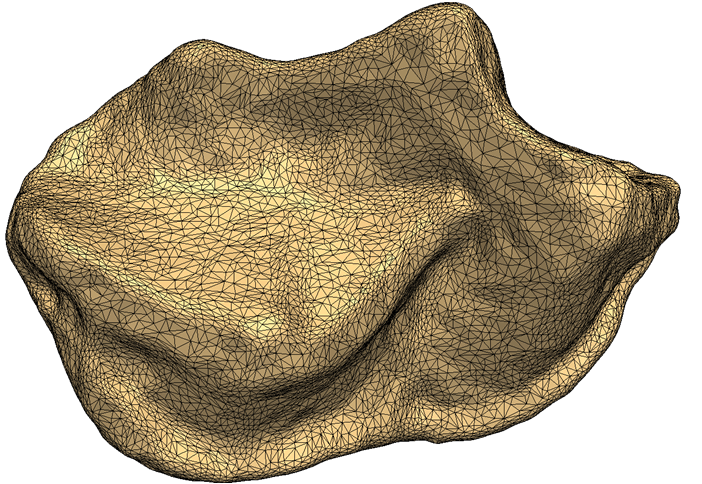
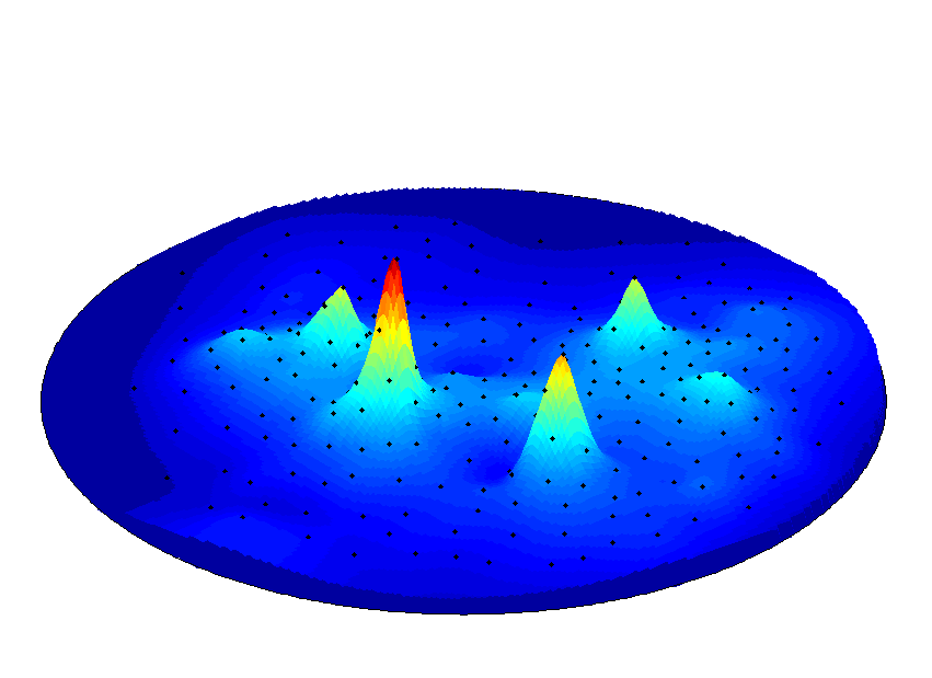
The discrete representation of a surface (mesh)	Conformal density over the unit disk

Figure 2. A mammalian tooth discrete surface mesh, and its approximated conformal factor over the unit disk.

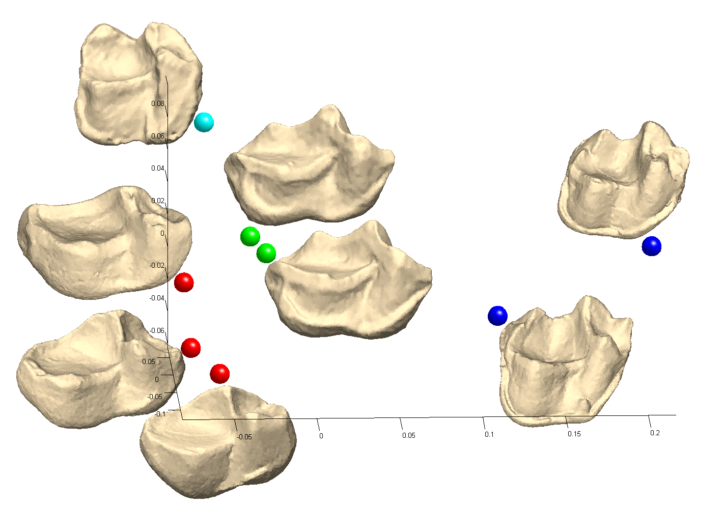
Figure 3. Embedding of the distance graph of eight teeth models using multi-dimensional scaling. Different colors represent different lemur species. The graph suggests that the geometry of the teeth might suffice to classify species.

5. Acknowledgments

The authors would like to thank Cédric Villani and Thomas Funkhouser for valuable discussions, and Jesus Puente for helping with the implementation. We are grateful to Jukka Jernvall, Stephen King, and Doug Boyer for providing us with the tooth data sets, and for many interesting comments. ID gratefully acknowledges (partial) support for this work by NSF grant DMS-0914892, and by an AFOSR Complex Networks grant; YL thanks the Rothschild foundation for postdoctoral fellowship support.

Appendix A

This Appendix contains some technical proofs of Lemmas and Theorems stated in section 3, and 4. We start by proving that (3.1) does indeed define a distance metric on the family of $\overline{\mu}:=\{m_{*}\mu\,;\,m\in M_{\mathcal{D}}\,\}$, where the $\mu$ are (smooth) conformal factors on $\mathcal{D}$, as obtained in sections 2 and 3. We first state a more general lemma:

Lemma A.1.

Let $X,\,d$ be a metric space, $G$ a group, and $T:\,g\,\mapsto\,T_{g}$ a representation of $G$ into the isometries of $X,\,d$; in particular, $d$ is invariant under the action of the group $G$, i.e. $d(T_{g}x,T_{G}y)\,=\,d(x,y)$, for all $x,\,y\in X$ and all $g\in G$. Define $\mathcal{C}$ to be the collection of orbits of the representation of $G$, i.e. the elements of $\mathcal{C}$ take of the form $\{T_{g}x\,;\,g\in G\}$, for some $x\in X$. Define $\widetilde{d}$ on $\mathcal{C}\times\mathcal{C}$ by $\widetilde{d}(c_{1},c_{2})=\inf_{x_{1}\in c_{1},\,x_{2}\in c_{2}}d(x_{1},x_{2})$. Then $\widetilde{d}$ defines a semi-metric on $\mathcal{C}$.

Proof.

It is obvious that $\widetilde{d}(c_{1},c_{2})\geq 0$ for all $c_{1},\,c_{2}$ in $\mathcal{C}$; thus only the triangle inequality needs to be established.
Since an element $c_{1}$ of $\mathcal{C}$ can always be written as $c_{1}\,=\,\{T_{g}x;g\in G\}$, where $x$ is an arbitrary element of $G$, we obtain, for arbitrary $c_{1}$, $c_{2}$, $c_{3}$ in $\mathcal{C}$,

$$\widetilde{d}(c_{1},c_{3}) =\inf_{g,\,g^{\prime}\in G}d(T_{g}x,T_{g^{\prime}}z)~{}~{} \mbox{ where }x\in c_{1},\,z\in c_{3}\mbox{ are arbitrary}$$

$$\leq d(T_{g_{1}}x,T_{g_{3}}z)~{}~{} \mbox{ for all }g_{1},\,g_{3}\in G$$

$$\leq d(T_{g_{1}}x,T_{g_{2}}y)\,+\,d(T_{g_{2}}y,T_{g_{3}}z)~{}~{} \mbox{ for all }g_{1},\,g_{2},\,g_{3}\in G\mbox{ and all }y\in X$$

$$=d(T_{g_{1}}x,T_{g_{2}}y)\,+\,d(T_{g^{\prime}_{2}}y,T_{g^{\prime}_{2}(g_{2})^{-1}g_{3}}z)~{}~{} \mbox{ for all }g_{1},\,g_{2},\,g^{\prime}_{2},\,g_{3}\in G\mbox{ and all }y\in X.$$

When $g^{\prime}_{2},\,g_{2}$ in $G$ are kept fixed, the group elements $g^{\prime}_{2}(g_{2})^{-1}g_{3}$ run through all of $G$ as $g_{3}$ varies over $G$. By taking the infimum over the choices of $g_{1},\,g_{2},\,g^{\prime}_{2},\,g_{3}\in G$ in the last expression, we thus obtain

$$\widetilde{d}(c_{1},c_{3})\leq\widetilde{d}(c_{1},c_{2})\,+\,\widetilde{d}(c_{2},c_{3})~{},$$

where $c_{2}:=\{T_{g}y\,;\,g\in G\}$. Since $y\in X$ is arbitrary, this proves the triangle inequality in $\mathcal{C}$ for all three-tuples in $\mathcal{C}$. ∎

Note that one can use the invariance of $d$ under the action of the group on $X$ to define $\widetilde{d}(c_{1},c_{2})$ via a single minimization (instead of two): for $x\in c_{1}$, $y\in c_{2}$,

$$\widetilde{d}(c_{1},c_{2})\,=\,\inf_{g,\,g^{\prime}\in G}\,d(T_{g}x,T_{g^{\prime}}y)\,=\,\inf_{g,\,g^{\prime}\in G}\,d(x,T_{g^{-1}g^{\prime}}y)\,=\,\inf_{g^{\prime\prime}\in G}\,d(x,T_{g^{\prime\prime}}y)~{}.$$

To apply this to (3.1), we choose $X$ to be the set of nonnegative $C^{1}$-functions on $\mathcal{D}$ that have integral 1 with respect to the hyperbolic area measure on $\mathcal{D}$, and $d$ the Kantorovich mass transport distance between them, with the “work” measured in terms of the hyperbolic distance metric $d^{\mbox{\tiny{H}}}$ on $\mathcal{D}$:

$$\mbox{d}(\mu,\nu)\,=\,\inf_{\pi\in\Pi(\mu,\nu)}\,\int_{\mathcal{D}\times\mathcal{D}}\,d^{\mbox{\tiny{H}}}(z,w)\,d\pi(z,w)\,.$$

The group $G$ is here given by $M_{\mathcal{D}}$, and the action of $G$ on $X$ by pull-back: $T_{m}(\mu)\,=\,m_{*}\mu$. To apply the lemma, we first need to establish that :

Lemma A.2.

$\mbox{\rm{d}}(\mu,\nu)\,=\,\mbox{\rm{d}}(m_{*}\mu,m_{*}\nu)$, for all $\mu$, $\nu$ in $X$, and all $m$ in $M_{\mathcal{D}}$.

Proof.

We first rewrite $\mbox{d}(m_{*}\mu,m_{*}\nu)$ in a different way. For each $\pi\in\Pi(\mu,\nu)$, we define the probability measure $m_{*}\pi$ on $\mathcal{D}\times\mathcal{D}$ by $m_{*}\pi(E)\,=\,\pi\left(\,\{\,(m^{-1}z,m^{-1}w)\,;\,(z,w)\in E\,\}\,\right)$. It is straightforward to check that $m_{*}\pi(A\times\mathcal{D})\,=\,m_{*}\mu(A)$ and $m_{*}\pi(\mathcal{D}\times B)\,=\,m_{*}\nu(B)$ for all Borel sets $A$ , $B\subset\mathcal{D}$; thus $m_{*}\pi\in\Pi(m_{*}\mu,m_{*}\nu)$. One can analogously define $m^{*}\pi$; again it is straightforward that $m^{*}m_{*}\pi\,=\,\pi$. It follows that $\Pi(m_{*}\mu,m_{*}\nu)$ is exactly equal to $\{\,m_{*}\pi\,;\,\pi\in\Pi(\mu,\nu)\,\}$.

Consequently, using the invariance $d^{\mbox{\tiny{H}}}(mz,mw)\,=\,d^{\mbox{\tiny{H}}}(z,w)$, we obtain

$$\mbox{d}(m_{*}\mu,m_{*}\nu)\, =\,\inf_{\pi\in\Pi(\mu,\nu)}\,\int_{\mathcal{D}\times\mathcal{D}}\,d^{\mbox{\tiny{H}}}(z,w)\,d(m_{*}\pi)(z,w)=\inf_{\pi\in\Pi(\mu,\nu)}\,\int_{\mathcal{D}\times\mathcal{D}}\,d^{\mbox{\tiny{H}}}(mu,mv)\,d\pi(u,v)$$

$$=\inf_{\pi\in\Pi(\mu,\nu)}\,\int_{\mathcal{D}\times\mathcal{D}}\,d^{\mbox{\tiny{H}}}(u,v)\,d\pi(u,v)\,=\,\mbox{d}(\mu,\nu)~{}.$$

∎

It follows that we can indeed apply the first lemma, and that (3.1) defines a semi-metric on the equivalence classes of conformal factors, where two conformal factors are viewed as equivalent if one can be obtained from the other by pushing it forward (or backward) through a Möbius transformation.

It turns out that in this case, the infimum over the choices $m\in M_{\mathcal{D}}$ is in fact always achieved (and is thus a minimum):

Lemma A.3.

Let $\mu$ and $\nu$ be conformal factors obtained by uniformizing two smooth disk-type surfaces, with $\mbox{Distance}(\mu,\nu)<\infty$ defined as in (3.1). Then there exists a Möbius transformation $m\in M_{\mathcal{D}}$ such that $\mbox{Distance}(\mu,\nu)\,=\,\mbox{\rm{d}}(m_{*}\mu,\nu)$.

Proof.

Consider two arbitrary (but fixed) conformal factors $\mu$ and $\nu$ on $\mathcal{D}$. There exists a sequence $\left(m_{n}\right)_{n\in\mathbb{N}}$ such that $\inf_{\pi\in\Pi(\mu,\nu)}\,\int_{\mathcal{D}\times\mathcal{D}}\,d^{\mbox{\tiny{H}}}(m_{n}(z),w)\,d\pi(z,w)$ $\rightarrow\mbox{Distance}(\mu,\nu)\,$ as $n\,\rightarrow\,\infty$. Each of these $m_{n}$ can be written in the form given by (2.3), with corresponding $a_{n}\in\mathcal{D}$, and $e^{i\theta_{n}}\in\mathbb{T}:=\{\,z\in\mathbb{C}\,;\,|z|=1\,\}$. By passing to a subsequence if necessary, we can assume, without loss of generality, that the sequences $\left(a_{n}\right)_{n\in\mathbb{N}}$ and $\left(e^{i\theta_{n}}\right)_{n\in\mathbb{N}}$ converge in $\overline{\mathcal{D}}$ (the closure of $\mathcal{D}$) and $\mathbb{T}$, respectively, to limits we denote by $\overline{a}$ and $e^{i\overline{\theta}}$.

If $\overline{a}$ lies in the open disk $\mathcal{D}$, then it defines, together with $e^{i\overline{\theta}}$, a corresponding $\overline{m}\in M_{\mathcal{D}}$. We then have, for all $z,\,w$ in $\mathcal{D}$, $\lim_{n\rightarrow\infty}\,d^{\mbox{\tiny{H}}}(m_{n}(z),w)\,=\,d^{\mbox{\tiny{H}}}(\overline{m}(z),w)$. On the other hand, for sufficiently large $n$ we have

$$d^{\mbox{\tiny{H}}}(m_{n}(z),w) \leq d^{\mbox{\tiny{H}}}(m_{n}(z),0)\,+\,d^{\mbox{\tiny{H}}}(0,w)$$

$$= d^{\mbox{\tiny{H}}}(z,a_{n})\,+\,d^{\mbox{\tiny{H}}}(0,w)$$

$$\leq d^{\mbox{\tiny{H}}}(z,\overline{a})\,+1\,+\,d^{\mbox{\tiny{H}}}(0,w)$$

$$\leq d^{\mbox{\tiny{H}}}(z,0)\,+\,d^{\mbox{\tiny{H}}}(0,\overline{a})\,+1\,+\,d^{\mbox{\tiny{H}}}(0,w),$$

where we have used the invariance of $d^{\mbox{\tiny{H}}}$ under Möbius transformations and $m_{n}(a_{n})=0$ in the second line, and where we assume $n$ sufficiently large to ensure $d^{\mbox{\tiny{H}}}(a_{n},\overline{a})\leq 1$ in the third.

Therefore $d^{\mbox{\tiny{H}}}(m_{n}(z),w)$ is bounded, uniformly in $n$, by a function that is absolutely integrable with respect to $\pi$ (by the argument used just before the statement of Lemma A.2); the dominated convergence theorem then implies that

$$\mbox{\hausaD}(\mu,\nu) = \lim_{n\rightarrow\infty}\,\int_{\mathcal{D}\times\mathcal{D}}\,d^{\mbox{\tiny{H}}}(m_{n}(z),w)\,d\pi(z,w)$$

$$= \int_{\mathcal{D}\times\mathcal{D}}\,d^{\mbox{\tiny{H}}}(\overline{m}(z),w)\,d\pi(z,w)\,,$$

so that we are done for the case where $\overline{a}\in\mathcal{D}$.

It remains to discuss the case where $\overline{a}\in\overline{\mathcal{D}}\setminus\mathcal{D}=\mathbb{T}$, i.e. $|a|\,=\,1$. The proof will be complete if we show that this is impossible; we will establish this by contradiction.

From now on, we suppose that $|\overline{a}|=1$. By the integrability of $\mu$ and $\nu$, we can find an increasing sequence of $\rho_{n}<1$ such that $\mu\left(\{z\,;\,1>|z|>\rho_{n}\,\}\right)<1/n$ and $\nu\left(\{z\,;\,1>|z|>\rho_{n}\,\}\right)<1/n$ . It is easy to check that

$$\mbox{for }|a|>R\mbox{ and }|z|<\rho<R\mbox{ : }\left|\frac{z-a}{1-a^{*}z}\right|>\frac{R-\rho}{1-R\rho}~{}.$$

This lower bound tends to 1 as $R$ tends to 1, regardless of the value of $\rho<1$. It follows that there exist $R_{n}<1$ so that

$$\inf_{|z|<\rho_{n}}\left|\frac{z-a}{1-a^{*}z}\right|>(n+\rho_{n})/(n+1),~{}\mbox{ for all }a\mbox{ with }|a|>R_{n}~{}.$$

Because $|\overline{a}|=1$, we can find a $k_{n}\in\mathbb{N}$ such that $|a_{k}|>R_{n}$ for all $k>k_{n}$; consequently $|m_{k}(z)|\,=\,|z-a_{k}|/|1-(a_{k})^{*}z|>(n+\rho_{n})/(n+1)\,$ for all $k>k_{n}$ and all $z$ with $|z|<\rho_{n}$. It then follows that (with the notation $\mathcal{D}_{n}\,:=\,\{\,z\,;\,|z|<\rho_{n}\,\}$)

$$\forall k>k_{n}\,,\,\forall\pi\in\Pi(\mu,\nu):\,\int_{\mathcal{D}\times\mathcal{D}}\, d^{\mbox{\tiny{H}}}(m_{k}(z),w)\,d\pi(z,w)$$

$$\geq\int_{\mathcal{D}_{n}\times\mathcal{D}_{n}}\,d^{\mbox{\tiny{H}}}(m_{k}(z),w)\,d\pi(z,w)$$

$$\geq\int_{\mathcal{D}_{n}\times\mathcal{D}_{n}}\,\left[\,\inf_{|v|<\rho_{n},\,|u|>(n+\rho_{n})/(n+1))}d^{\mbox{\tiny{H}}}(u,v)\,\right]\,d\pi(z,w)$$

$$\geq\frac{\ln(n+1)}{2}\,\int_{\mathcal{D}_{n}\times\mathcal{D}_{n}}\,d\pi(z,w)$$

$$\geq\frac{\ln(n+1)}{2}\,\left[\,1\,-\,\pi((\mathcal{D}\setminus\mathcal{D}_{n})\times\mathcal{D})\,-\,\pi(\mathcal{D}\times(\mathcal{D}\setminus\mathcal{D}_{n}))\,\right]$$

$$\geq\frac{\ln(n+1)}{2}\,\left(\,1\,-\,\frac{2}{n}\,\right)~{},$$

where we have used that if $|u|<r<1$, and $|v|>(n+r)/(n+1)$, then $d^{\mbox{\tiny{H}}}(u,v)\geq\int_{r}^{(n+r)/(1+n)}\,\frac{1}{1-t^{2}}\,dt\geq\frac{1}{2}\,\int_{r}^{(n+r)/(1+n)}\,\frac{1}{1-t}\,dt\,=\,\frac{\ln(n+1)}{2}$ . This shows, in particular, that

$$\mbox{\rm{d}}(\mu,m_{k}^{*}\nu)\,=\,\inf_{\pi\in\Pi(\mu,\nu)}\,\int_{\mathcal{D}\times\mathcal{D}}\,d^{\mbox{\tiny{H}}}(m_{k}(z),w)\,d\pi(z,w)\geq\frac{\ln(n+1)}{4}$$

for all $k>k_{n}$ and $n>4$. This implies that, for arbitrary $n>4,\,n\in\mathbb{N}$,

$$\mbox{Distance}(\mu,\nu)\,=\,lim_{k\rightarrow\infty}\,\mbox{\rm{d}}(\mu,m_{k}^{*}\nu)\geq\frac{\ln(n+1)}{4}\,,$$

i.e. $\mbox{Distance}(\mu,\nu)\,=\,\infty$, a contradiction. This finishes the argument that $|\overline{a}|=1$ is not possible, and completes the proof. ∎

It is now easy to see that $\mbox{Distance}(\mu,\nu)$ defines a true metric on the equivalence classes of conformal factors:

Proposition A.4.

The $\mbox{Distance}(\mu,\nu)$ defined in (3.1) is a metric on the set of orbits $\overline{\mu}:=\{m_{*}\mu\,;\,m\in M_{\mathcal{D}}\,\}$ of conformal factors under the action of $M_{\mathcal{D}}$.

Proof.

In view of the first lemma, we need to prove only that $\mbox{Distance}(\mu,\nu)=0$ implies that there exists a Möbius transformation $m\in M_{\mathcal{D}}$ such that $\nu=m_{*}\mu$. By the second lemma, we know that $\mbox{Distance}(\mu,\nu)=\rm{d}(m_{*}\mu,\nu)$ for some $m\in M_{\mathcal{D}}$. For this $m$ there exist thus $\pi_{k}\in\Pi(\mu,\nu)$ such that $\int_{\mathcal{D}\times\mathcal{D}}\,d^{\mbox{\tiny{H}}}(m(z),w)\,d\pi_{k}(z,w)$ tends to 0 as $k$ tends to $\infty$. By passing to a subsequence if necessary, we can, using the weak$*$-compactness of the set of probability measures on $\mathcal{D}\times\mathcal{D}$, assume that $\pi_{k}\rightarrow\overline{\pi}$ as $k$ tends to infinity, in the weak$*$-topology, where $\overline{\pi}$ is a measure of weight at most 1. Since the $\pi_{k}$ all have marginals $\mu$ and $\nu$, respectively, it follows that $\overline{\pi}$ must have these marginals as well, which guarantees that $\overline{\pi}$ is itself a probability measure and an element of $\Pi(\mu,\nu)$. We have moreover

$$0\,=\,\mbox{Distance}(\mu,\nu)\,=\,\int_{\mathcal{D}\times\mathcal{D}}\,d^{\mbox{\tiny{H}}}(m(z),w)\,d\overline{\pi}(z,w)~{},$$

implying that the support of $\overline{\pi}$ is contained in the subset $\{\,(z,m(z))\,;\,z\in\mathcal{D}\,\}\subset\mathcal{D}\times\mathcal{D}$. It then follows that, for any Borel set $A\subset\mathcal{D}$,

$$\int_{A}\,\mu(z)\,d\mbox{\rm{\footnotesize{vol}}}_{H}(z)\,=\,\overline{\pi}(A\times\mathcal{D})\,=\,\overline{\pi}(A\times m(A))\,=\,\overline{\pi}(\mathcal{D}\times m(A))\,=\,\int_{A}\,\nu(m(z))\,d\mbox{\rm{\footnotesize{vol}}}_{H}(z)~{}.$$

This is possible for the continuous functions $\mu$ and $\nu$ only if $\nu=m^{*}\mu$, or equivalently, $\mu=m_{*}\nu$

∎

Next we prove the list of properties of the distance function $d^{R}_{\mu,\nu}(z,w)$ given in Theorem 3.3:

Theorem 3.3

The distance function $d^{R}_{\mu,\nu}(z,w)$ satisfies the following properties

(1)	$~{}d^{R}_{m^{*}_{1}\mu,m^{*}_{2}\nu}(m^{-1}_{1}({z_{0}}),m^{-1}_{2}({w_{0}}))=d^{R}_{\mu,\nu}({z_{0}},{w_{0}})~{}$	Invariance under (well-defined)
		Möbius changes of coordinates
(2)	$~{}d^{R}_{\mu,\nu}({z_{0}},{w_{0}})=d^{R}_{\nu,\mu}({w_{0}},{z_{0}})~{}$	Symmetry
(3)	$~{}d^{R}_{\mu,\nu}({z_{0}},{w_{0}})\geq 0~{}$	Non-negativity
(4)	$\!\!\!\!\!\!~{}d^{R}_{\mu,\nu}({z_{0}},{w_{0}})=0\,\Longrightarrow\,\Omega_{z_{0},R}$ in $(\mathcal{D},\mu)$ and $\Omega_{w_{0},R}$ in $(\mathcal{D},\nu)$ are isometric
(5)	$~{}d^{R}_{m^{*}\nu,\nu}(m^{-1}({z_{0}}),{z_{0}})=0~{}$	Reflexivity
(6)	$~{}d^{R}_{\mu_{1},\mu_{3}}(z_{1},z_{3})\leq d^{R}_{\mu_{1},\mu_{2}}(z_{1},z_{2})+d^{R}_{\mu_{2},\mu_{3}}(z_{2},z_{3})~{}$	Triangle inequality

Proof.

For (1), denote $m_{1}^{-1}(z_{0})=z_{1}$, and $m_{2}^{-1}(w_{0})=w_{1}$. Then

$$d^{R}_{m_{1}^{*}\mu,m_{2}^{*}\nu}(z_{1},w_{1}) =\mathop{\inf}_{m(z_{1})=w_{1}}\int_{\Omega_{z_{1},R}}|m_{1}^{*}\mu(z)-m^{*}m_{2}^{*}\nu(z)|d\mbox{\rm{\footnotesize{vol}}}_{H}(z)$$

$$=\mathop{\inf}_{m(z_{1})=w_{1}}\int_{\Omega_{z_{1},R}}|\mu(m_{1}(z))-\nu(m_{2}(m(z)))|d\mbox{\rm{\footnotesize{vol}}}_{H}(z).$$

Next set $\widetilde{m}=m_{2}\circ m\circ m_{1}^{-1}$. Note that $\widetilde{m}(z_{0})=w_{0}$. Plugging $m_{2}(m(z))=\widetilde{m}(m_{1}(z))$ into the integral and carrying out the change of variables $m_{1}(z)=z^{\prime}\,$, we obtain

$$\mathop{\inf}_{m(z_{1})=w_{1}}\int_{\Omega_{z_{1},R}}|\,\mu(z^{\prime})-\nu(\widetilde{m}(z^{\prime}))\,|d\mbox{\rm{\footnotesize{vol}}}_{H}(z^{\prime})=\mathop{\inf}_{\widetilde{m}(z_{0})=w_{0}}\int_{\Omega_{z_{0},R}}|\,\mu(z^{\prime})-\nu(\widetilde{m}(z^{\prime}))\,|\,d\mbox{\rm{\footnotesize{vol}}}_{H}(z^{\prime}).$$

For (2), we use Lemma 3.2 and equations (2.5), (2.6) to write

$$d^{R}_{\mu,\nu}(z_{0},w_{0}) =\mathop{\inf}_{m(z_{0})=w_{0}}\int_{\Omega_{z_{0}},R}|\mu(z)-m^{*}\nu(z)|d\mbox{\rm{\footnotesize{vol}}}_{H}(z)$$

$$=\mathop{\inf}_{m(z_{0})=w_{0}}\int_{\Omega_{w_{0}},R}|(m^{-1})^{*}\mu(w)-\nu(w)|d\mbox{\rm{\footnotesize{vol}}}_{H}(w)=d^{R}_{\nu,\mu}(w_{0},z_{0}).$$

(3) and (4) are immediate from the definition of $d^{R}_{\mu,\nu}$.

(5) follows from the observation that the minimizing $m$ (in the definition (3.5) of $d^{R}_{\mu,\nu}$) is $m_{1}$ itself, for which the integrand, and thus the whole integral vanishes identically.

For (6), let $m_{1}$ be a Möbius transformation such that $m_{1}(z_{1})=z_{2}$, and $m_{2}$ such that $m_{2}(z_{2})=z_{3}$. Setting $m=m_{2}\circ m_{1}$, we have

$$d^{R}_{\mu_{1},\mu_{3}}(z_{1},z_{3}) \leq\int_{\Omega_{z_{1},R}}|\,\mu_{1}(z)-m^{*}\mu_{3}(z)\,|\,d\mbox{\rm{\footnotesize{vol}}}_{H}(z)$$

(A.1) $$\leq\int_{\Omega_{z_{1},R}}|\,\mu_{1}(z)-m_{1}^{*}\mu_{2}(z)\,|\,d\mbox{\rm{\footnotesize{vol}}}_{H}(z)+\int_{\Omega_{z_{1},R}}|\,m_{1}^{*}\mu_{2}(z)-m^{*}\mu_{3}(z)\,|\,d\mbox{\rm{\footnotesize{vol}}}_{H}(z)\,.$$

The second term in (A.1) can be rewritten as (using Lemma 3.2, the change of coordinates $m_{1}(z_{1})=z_{2}$ and the observation $m^{*}=m_{1}^{*}m_{2}^{*}$)

$$\int_{\Omega_{z_{1},R}}|\,m_{1}^{*}\mu_{2}(z)-m^{*}\mu_{3}(z)\,|\,d\mbox{\rm{\footnotesize{vol}}}_{H}(z) =\int_{\Omega_{z_{2},R}}|\,m_{1*}m_{1}^{*}\mu_{2}(w)-m_{1*}m_{1}^{*}m_{2}^{*}\mu_{3}(w)\,|\,d\mbox{\rm{\footnotesize{vol}}}_{H}(w)$$

$$=\int_{\Omega_{z_{2},R}}|\,\mu_{2}(w)-m_{2}^{*}\mu_{3}(w)\,|\,d\mbox{\rm{\footnotesize{vol}}}_{H}(w).$$

We have thus

$$d^{R}_{\mu_{1},\mu_{3}}(z_{1},z_{3})\leq\int_{\Omega_{z_{1},R}}|\,\mu_{1}(z)-m_{1}^{*}\mu_{2}(z)\,|\,d\mbox{\rm{\footnotesize{vol}}}_{H}(z)+\int_{\Omega_{z_{2},R}}|\,\mu_{2}(w)-m_{2}^{*}\mu_{3}(w)\,|\,d\mbox{\rm{\footnotesize{vol}}}_{H}(w)~{},$$

and this for any $m_{1},\,m_{2}\in M_{\mathcal{D}}$ such that $m_{1}(z_{1})=z_{2}$ and $m_{2}(z_{2})=z_{3}$. Minimizing over $m_{1}$ and $m_{2}$ then leads to the desired result.

∎

Next we prove the continuity properties of the function $\Phi(z_{0},w_{0},\sigma)=\int_{\Omega(z_{0},R)}\,|\,\mu(z)-\nu(m_{z_{0},w_{0},\sigma}(z))\,|\,d\mbox{\rm{\footnotesize{vol}}}_{H}(z)$, stated in Lemma 3.6, which were used to prove continuity of $d^{R}_{\mu,\nu}$ itself (in Theorem 3.7).

Lemma 3.6
$\bullet$ For each fixed $(z_{0},w_{0})$ the function $\Phi(z_{0},w_{0},\cdot)$ is continuous on $S_{1}$.
$\bullet$ For each fixed $\sigma\in S_{1}$, $\Phi(\cdot,\cdot,\sigma)$ is continuous on $\mathcal{D}\times\mathcal{D}$. Moreover, the family $\Big{(}\Phi(\cdot,\cdot,\sigma)\Big{)}_{\sigma\in S_{1}}$ is equicontinuous.

Proof.

We start with the continuity in $\sigma$. We have

$$\left|\,\Phi(z_{0},w_{0},\sigma)-\Phi(z_{0},w_{0},\sigma^{\prime})\,\right|\leq\int_{\Omega(z_{0},R)}\,|\nu(m_{z_{0},w_{0},\sigma}(z))-\nu(m_{z_{0},w_{0},\sigma^{\prime}}(z))\,|\,d\mbox{\rm{\footnotesize{vol}}}_{H}(z)~{}.$$

Because $\nu$ is continuous on $\mathcal{D}$, its restriction to the compact set $\overline{\Omega(w_{0},R)}$ (the closure of $\Omega(w_{0},R)$) is bounded. Since the hyperbolic volume of $\Omega(z_{0},R)$ is finite, the integrand is dominated, uniformly in $\sigma^{\prime}$, by an integrable function. Since $m_{z_{0},w_{0},\sigma}(z)$ is obviously continuous in $\sigma$, we can use the dominated convergence theorem to conclude.

Since $S^{1}$ is compact, this continuity implies that the infimum in the definition of $d^{R}_{\mu,\nu}$ can be replaced by a minimum:

$$d^{R}_{\mu,\nu}(z_{0},w_{0})=\mathop{\min}_{m(z_{0})=w_{0}}\,\int_{\Omega(z_{0},R)}\,|\,\mu(z)-\nu(m(z))\,|\,d\mbox{\rm{\footnotesize{vol}}}_{H}(z)~{}.$$

Next we prove continuity in $z_{0}$ and $w_{0}$ (with estimates that are uniform in $\sigma$).

Consider two pairs of points, $(z_{0},w_{0})$ and $(z^{\prime}_{0},w^{\prime}_{0})\in\mathcal{D}\times\mathcal{D}$. Then

$$|\,\Phi(z_{0},w_{0},\sigma)-\Phi(z^{\prime}_{0},w^{\prime}_{0},\sigma)\,|$$

$$~{}~{}~{}~{}~{}=\,\left|\,\int_{\Omega(z_{0},R)}\,|\,\mu(z)-\nu(m_{z_{0},w_{0},\sigma}(z))\,|\,d\mbox{\rm{\footnotesize{vol}}}_{H}(z)-\int_{\Omega(z^{\prime}_{0},R)}\,|\,\mu(u)-\nu(m_{z^{\prime}_{0},w^{\prime}_{0}\sigma}(u)\,|\,d\mbox{\rm{\footnotesize{vol}}}_{H}(u)\,\right|$$

$$~{}~{}~{}~{}~{}\leq\,\left|\,\int_{\Omega(z_{0},R)}\,|\,\mu(z)-\nu(m_{z_{0},w_{0},\sigma}(z))\,|\,d\mbox{\rm{\footnotesize{vol}}}_{H}(z)-\int_{\Omega(z_{0},R)}\,|\,\mu(m_{z_{0},z^{\prime}_{0},1}z)-\nu(m_{z^{\prime}_{0},w^{\prime}_{0},\sigma}\circ m_{z_{0},z^{\prime}_{0},1}(z))\,|\,d\mbox{\rm{\footnotesize{vol}}}_{H}(u)\,\right|$$

$$~{}~{}~{}~{}~{}\leq\int_{\Omega(z_{0},R)}\,\left(\,|\,\mu(z)-\mu(m_{z_{0},z^{\prime}_{0},1}(z))\,|+|\,\nu(m_{z_{0},w_{0},\sigma}(z))-\nu(m_{z^{\prime}_{0},w^{\prime}_{0},\sigma}(m_{z_{0},z^{\prime}_{0},1}(z)))\,|\,\right)\,d\mbox{\rm{\footnotesize{vol}}}_{H}(z)~{}.$$

On the other hand, note that for any $\gamma>0$, $\mu$ and $\nu$ are continuous on the closures of $\Omega(z_{0},R+\gamma)$ and $\Omega(w_{0},R+\gamma)$, respectively; since these closed hyperbolic disks are compact, $\mu$ and $\nu$ are bounded on these sets. Pick now $\rho>0$ such that $|z^{\prime}_{0}-z_{0}|<\rho$, $|w^{\prime}_{0}-w_{0}|<\rho$ imply that $\Omega(z^{\prime}_{0},R)\subset\Omega(z_{0},R+\gamma)$ as well as $\Omega(w^{\prime}_{0},R)\subset\Omega(w_{0},R+\gamma)$. It follows that, if $|z^{\prime}_{0}-z_{0}|<\rho$ and $|w^{\prime}_{0}-w_{0}|<\rho$, then $|\,\mu(z)-\mu(m_{z_{0},z^{\prime}_{0},1}(z)\,|$ and $|\,\nu(m_{{z_{0}}_{0},w_{0},\sigma}(z))-\nu(m_{z^{\prime}_{0},w^{\prime}_{0},\sigma}(m_{z_{0},z^{\prime}_{0},1}(z)))\,|$ are bounded uniformly for $z\in\Omega(z_{0},R)$. Since it is clear from the explicit expressions (3.7) that $m_{z_{0},z^{\prime}_{0},1}(z)\rightarrow z$ and $m_{z^{\prime}_{0},w^{\prime}_{0},\sigma}(m_{z_{0},z^{\prime}_{0},1}(z))\rightarrow m_{z_{0},w_{0},\sigma}(z)$ as $z^{\prime}_{0}\rightarrow z_{0}$ and $w^{\prime}_{0}\rightarrow w_{0}$, we can thus invoke the dominated convergence theorem again to prove continuity of $\Phi(\cdot,\cdot,\sigma)$.

To prove the equicontinuity, we first note that $\nu$ is uniformly continuous on $\Omega(w_{0},R)\cup\Omega(w^{\prime}_{0},R)$, since $\nu$ is continuous on the compact set $\overline{\Omega(w_{0},R+\gamma)}$, which contains $\Omega(w_{0},R)\cup\Omega(w^{\prime}_{0},R)$ for all $w^{\prime}_{0}$ that satisfy $|w^{\prime}_{0}-w_{0}|\leq\rho$. This means that, given any $\varepsilon>0$, we can find $\delta>0$ such that $|\nu(w)-\nu(w^{\prime})|\leq\varepsilon$ holds for all $w,\,w^{\prime}$ that satisfy $w,\,w^{\prime}\in\Omega(w_{0},R)\cup\Omega(w^{\prime}_{0},R)$ and $|w-w^{\prime}|\leq\delta$. This implies the desired equicontinuity if we can show that $|m_{z_{0},w_{0},\sigma}(z)-m_{z^{\prime}_{0},w^{\prime}_{0},\sigma}(m_{z_{0},z^{\prime}_{0},1}(z))|$ can be made smaller than $\delta$, uniformly in $\sigma\in S_{1}$, by making $|z^{\prime}_{0}-z_{0}|+|w^{\prime}_{0}-w_{0}|$ sufficiently small.
We first estimate $|m_{z_{0},w_{0},\sigma}(z)-m_{z_{0},w^{\prime}_{0},\sigma}(z)|$. With the notations of (3.7), we have

$$a(z_{0},w_{0},\sigma)-a(z_{0},w^{\prime}_{0},\sigma) =\frac{(z_{0}-w_{0}\overline{\sigma})(1-\overline{z_{0}}w^{\prime}_{0}\overline{\sigma})-(z_{0}-w^{\prime}_{0}\overline{\sigma})(1-\overline{z_{0}}w_{0}\overline{\sigma})}{(1-\overline{z_{0}}w_{0}\overline{\sigma})(1-\overline{z_{0}}w^{\prime}_{0}\overline{\sigma})}$$

$$=\frac{(w_{0}-w^{\prime}_{0})\overline{\sigma}(|z_{0}|^{2}-1)}{(1-\overline{z_{0}}w_{0}\overline{\sigma})(1-\overline{z_{0}}w^{\prime}_{0}\overline{\sigma})}~{},$$

so that

$$|a(z_{0},w_{0},\sigma)-a(z_{0},w^{\prime}_{0},\sigma)|\leq\frac{|w_{0}-w^{\prime}_{0}|}{(1-|z_{0}|\,|w_{0}|)[1-|z_{0}|(|w_{0}|+\xi)]}\leq\frac{\xi}{(1-|z_{0}|\,|w_{0}|)[1-|z_{0}|(|w_{0}|+\xi)]}$$

when $|w_{0}-w^{\prime}_{0}|<\xi$. It thus suffices to choose $\xi$ so that $\xi<\zeta(1-|z_{0}|\,|w_{0}|)[1-|z_{0}|(|w_{0}|+\xi)]$ to ensure that $|a(z_{0},w_{0},\sigma)-a(z_{0},w^{\prime}_{0},\sigma)|<\zeta$. For the phase factor $\tau$ in (3.7) we obtain

$$\tau(z_{0},w_{0},\sigma)-\tau(z_{0},w^{\prime}_{0},\sigma) =\sigma\,\frac{(1-\overline{z_{0}}w^{\prime}_{0}\overline{\sigma})(1-z_{0}\overline{w_{0}}\sigma)-(1-\overline{z_{0}}w_{0}\overline{\sigma})(1-z_{0}\overline{w^{\prime}_{0}}\sigma)}{(1-\overline{z_{0}}w_{0}\overline{\sigma})(1-\overline{z_{0}}w^{\prime}_{0}\overline{\sigma})}$$

$$=\sigma\,\frac{(w_{0}-w^{\prime}_{0})\overline{z_{0}}\overline{\sigma}-(\overline{w_{0}}-\overline{w^{\prime}_{0}})z_{0}\sigma+|z_{0}|^{2}(\overline{w_{0}}w^{\prime}_{0}-\overline{w^{\prime}_{0}}w_{0})}{(1-\overline{z_{0}}w_{0}\overline{\sigma})(1-\overline{z_{0}}w^{\prime}_{0}\overline{\sigma})}$$

$$=\sigma\,\frac{(w_{0}-w^{\prime}_{0})\overline{z_{0}}\overline{\sigma}-z_{0}(\overline{w_{0}}-\overline{w^{\prime}_{0}})\sigma+|z_{0}|^{2}[\overline{w_{0}}(w^{\prime}_{0}-w_{0})+w_{0}(\overline{w_{0}}-\overline{w^{\prime}_{0}}])}{(1-\overline{z_{0}}w_{0}\overline{\sigma})(1-\overline{z_{0}}w^{\prime}_{0}\overline{\sigma})}~{};$$

when $\left|w_{0}-w^{\prime}_{0}\right|<\xi$, this implies

$$|\tau(z_{0},w_{0},\sigma)-\tau(z_{0},w^{\prime}_{0},\sigma)|\leq\frac{|z_{0}|\,|w_{0}|\,[2+|z_{0}|(2|w_{0}|+\xi)]}{(1-|z_{0}|\,|w_{0}|)[1-|z_{0}|(|w_{0}|+\xi)]}\xi~{},$$

which can clearly be made smaller than any $\zeta>0$ by choosing $\xi$ sufficiently small. All this implies that (use (3.7))

$$|m_{z_{0},w_{0},\sigma}(z)-m_{z_{0},w^{\prime}_{0},\sigma}(z)| \leq|\tau(z_{0},w_{0},\sigma)-\tau(z_{0},w^{\prime}_{0},\sigma)|\frac{1+|z|}{1-|z|}\,+\,|a(z_{0},w_{0},\sigma)-a(z_{0},w^{\prime}_{0},\sigma)|\frac{(1+|z|)^{2}}{(1-|z|)^{2}}$$

$$\leq\zeta\,\frac{2(1+|z|)}{(1-|z|)^{2}},$$

which will be smaller than $\delta/2$, uniformly in $\sigma$, if $\zeta<\delta(1-|z|^{2})/8$; this bound on $\zeta$ in turn determines the bound to be imposed on the $\xi$ used above. Hence $|m_{z_{0},w_{0},\sigma}(z)-m_{z_{0},w^{\prime}_{0},\sigma}(z)|<\delta/2$ can be guaranteed, uniformly in $\sigma$, by choosing $|w_{0}-w^{\prime}_{0}|<\xi$ for sufficiently small $\xi$.
One can estimate likewise

$$|m_{z_{0},w^{\prime}_{0},\sigma}(z)-m_{z^{\prime}_{0},w^{\prime}_{0},\sigma}(m_{z^{\prime}_{0},z_{0},1}(z))|~{},$$

and show that this too can be made smaller than $\delta/2$, uniformly in $\sigma$, by imposing sufficiently tight bounds on $|z^{\prime}_{0}-z_{0}|$ and $|w^{\prime}_{0}-w_{0}|$. Combining all these estimates then leads to the desired equicontinuity, as indicated earlier. ∎

To prove Lemma 3.8, we shall use the following lemma:

Lemma A.5.

Consider $u_{k}=e^{\textbf{\footnotesize{i}}\psi}+\varepsilon_{k}$, where $\left|\varepsilon_{k}\right|\rightarrow 0$ as $k\rightarrow\infty$. Then there exists, for every $\varepsilon>0$, a $K\in\mathds{N}$ such that for all $k>K$; and all $\widehat{m}\in M_{D,0,u_{k}}$,

$$\inf_{w\in\Omega_{0,R}}\left|\widehat{m}(w)\right|>1-\varepsilon.$$

The set $M_{D,0,u_{k}}$ used in this lemma is given by Definition 3.4.

Proof.

From Lemma 3.5 we can write $\widehat{m}$ as

$$\widehat{m}(w)=e^{\textbf{\footnotesize{i}}\theta}\frac{w+u_{k}e^{-\textbf{\footnotesize{i}}\theta}}{1+\overline{u_{k}}e^{\textbf{\footnotesize{i}}\theta}w},$$

for some $\theta\in[0,2\pi)$. Substituting $u_{k}=e^{\textbf{\footnotesize{i}}\psi}+\varepsilon_{k}$ in this equation we get

$$\widehat{m}(w) =e^{\textbf{\footnotesize{i}}\theta}\frac{w+(e^{\textbf{\footnotesize{i}}\psi}+\varepsilon_{k})e^{-\textbf{\footnotesize{i}}\theta}}{1+\overline{(e^{\textbf{\footnotesize{i}}\psi}+\varepsilon_{k})}e^{\textbf{\footnotesize{i}}\theta}w}=e^{\textbf{\footnotesize{i}}\psi}\frac{1+we^{\textbf{\footnotesize{i}}(\theta-\psi)}+\varepsilon_{k}\varepsilon^{-\textbf{\footnotesize{i}}\psi}}{1+we^{\textbf{\footnotesize{i}}(\theta-\psi)}+\overline{\varepsilon_{k}}e^{\textbf{\footnotesize{i}}\theta}w}.$$

Writing the shorthand $s$ for $s=1+we^{\textbf{\footnotesize{i}}(\theta-\psi)}$, we have thus

$$\left|\widehat{m}(w)-e^{\textbf{\footnotesize{i}}\psi}\right| =\left|e^{\textbf{\footnotesize{i}}\psi}\frac{s+\varepsilon_{k}\varepsilon^{-\textbf{\footnotesize{i}}\psi}}{s+\overline{\varepsilon_{k}}e^{\textbf{\footnotesize{i}}\theta}w}-e^{\textbf{\footnotesize{i}}\psi}\right|\leq\left|e^{\textbf{\footnotesize{i}}\psi}\frac{\varepsilon_{k}e^{-\textbf{\footnotesize{i}}\psi}-\overline{\varepsilon}_{k}e^{\textbf{\footnotesize{i}}\theta}w}{s+\overline{\varepsilon}_{k}e^{\textbf{\footnotesize{i}}\theta}w}\right|$$

$$\leq\frac{\left|\varepsilon_{k}e^{-\textbf{\footnotesize{i}}\psi}-\overline{\varepsilon}_{k}e^{\textbf{\footnotesize{i}}\theta}w\right|}{\left|s+\overline{\varepsilon}_{k}e^{\textbf{\footnotesize{i}}\theta}w\right|}\leq\frac{\left|\varepsilon_{k}\right|\left(1+|w|\right)}{|s|-|\varepsilon_{k}||w|}$$

Now for all $w\in\Omega_{0,R}$, $|w|<r_{R}=\tanh^{-1}(R)$. This implies $|s|\geq 1-|w|\geq 1-r_{R}$, and $1+|w|\leq 1+r_{R}$, so that

$$\left|\widehat{m}(w)-e^{\textbf{\footnotesize{i}}\psi}\right|\leq|\varepsilon_{k}|\frac{1+r_{R}}{1-r_{R}-|\varepsilon_{k}|r_{R}}=|\varepsilon_{k}|\frac{1+r_{R}}{1-r_{R}\left(1+|\varepsilon_{k}|\right)}.$$

Since $\left|\varepsilon_{k}\right|\rightarrow 0$ the lemma follows. ∎

We are now ready for
Lemma 3.8 Let $\left\{(z_{k},w_{k})\right\}_{k\geq 1}\subset\mathcal{D}\times\mathcal{D}$ be a sequence that converges, in the Euclidean norm, to some point $(z^{\prime},w^{\prime})\in\overline{\mathcal{D}}\times\overline{\mathcal{D}}\setminus\mathcal{D}\times\mathcal{D}$, that is $|z_{k}-z^{\prime}|+|w_{k}-w^{\prime}|\rightarrow 0$, as $k\rightarrow\infty$. Then, $\lim_{k\rightarrow\infty}d^{R}_{\xi,\zeta}(z_{k},w_{k})$ exists and depends only on the limit point $(z^{\prime},w^{\prime})$.

Proof.

Since $(z^{\prime},w^{\prime})\in\overline{\mathcal{D}}\times\overline{\mathcal{D}}\setminus\mathcal{D}\times\mathcal{D}$ either $z^{\prime}\in\overline{\mathcal{D}}\setminus\mathcal{D}$ or $w^{\prime}\in\overline{\mathcal{D}}\setminus\mathcal{D}$. Let us assume that $z^{\prime}\in\overline{\mathcal{D}}\setminus\mathcal{D}$ (the case $w^{\prime}\in\overline{\mathcal{D}}\setminus\mathcal{D}$ is similar). Denote by $m_{k}$ an arbitrary Möbius transformation in $M_{D,0,w_{k}}$. By symmetry of the distance and using a change of variables we then obtain

$$d^{R}_{\xi,\zeta}(z_{k},w_{k}) =d^{R}_{\zeta,\xi}(w_{k},z_{k})$$

$$=\min_{m(w_{k})=z_{k}}\int_{\Omega_{w_{k},R}}\Big{|}\zeta(w)-\xi(m(w))\Big{|}d\mbox{\rm{\footnotesize{vol}}}_{H}(w)$$

$$=\min_{m(w_{k})=z_{k}}\int_{\Omega_{0,R}}\Big{|}\zeta(m_{k}(w))-\xi(m(m_{k}(w)))\Big{|}d\mbox{\rm{\footnotesize{vol}}}_{H}(w).$$

Now, recall that $\xi(z)=\xi^{H}(z)=\widetilde{\xi}(z)(1-|z|^{2})^{2}$, where $\widetilde{\xi}(z)$ is a bounded function, $\sup_{z\in\mathcal{D}}|\widetilde{\xi}(z)|\leq C_{\widetilde{\xi}}$. From Lemma A.5 we know that for every $\varepsilon>0$ and for $k>K$ sufficiently large, $\left|m(m_{k}((w))\right|>1-\varepsilon$ for all $w\in\Omega_{0,R}$, and all $m$ such that $m(w_{k})=z_{k}$. This means that for these $k>K$ we have

$$\left|\xi(m(m_{k}(w)))\right| =\left|\widetilde{\xi}(m(m_{k}(w)))\right|(1-\left|m(m_{k}(w))\right|^{2})^{2}$$

$$\leq C_{\widetilde{\xi}}(1-(1-\varepsilon)^{2})^{2}\leq C_{\widetilde{\xi}}\varepsilon^{2}(2-\varepsilon)^{2},$$

for all $w\in\Omega_{0,R}.$ Therefore,

$$\left|d^{R}_{\xi,\zeta}(z_{k},w_{k})-\int_{\Omega_{0,R}}\Big{|}\zeta(m_{k}(w))\Big{|}d\mbox{\rm{\footnotesize{vol}}}_{H}(w)\right|$$

$$\leq\left|\min_{m(w_{k})=z_{k}}\int_{\Omega_{0,R}}\Big{|}\zeta(m_{k}(w))-\xi(m(m_{k}(w)))\Big{|}d\mbox{\rm{\footnotesize{vol}}}_{H}(w)-\int_{\Omega_{0,R}}\Big{|}\zeta(m_{k}(w))\Big{|}d\mbox{\rm{\footnotesize{vol}}}_{H}(w)\right|$$

$$\leq\left|\min_{m(w_{k})=z_{k}}\int_{\Omega_{0,R}}\left\{\Big{|}\zeta(m_{k}(w))-\xi(m(m_{k}(w)))\Big{|}-\Big{|}\zeta(m_{k}(w))\Big{|}\right\}d\mbox{\rm{\footnotesize{vol}}}_{H}(w)\right|$$

$$\leq\min_{m(w_{k})=z_{k}}\int_{\Omega_{0,R}}\Big{|}\xi(m(m_{k}(w)))\Big{|}d\mbox{\rm{\footnotesize{vol}}}_{H}(w)\rightarrow 0,\ \mathrm{as}\ k\rightarrow\infty.$$

Therefore $d^{R}_{\xi,\zeta}(z_{k},w_{k})$ converges, as $k\rightarrow\infty$, if and only if $\int_{\Omega_{0,R}}\left|\zeta(m_{k}(w))\right|d\mbox{\rm{\footnotesize{vol}}}_{H}(w)$ converges, and to the same limit, for any $m_{k}\in M_{D,0,w_{k}}$. We can take, for instance, $m_{k}(w)=\frac{w+w_{k}}{1+\overline{w_{k}}w}$ which gives

$$\int_{\Omega_{0,R}}\left|\zeta(m_{k}(w))\right|d\mbox{\rm{\footnotesize{vol}}}_{H}(w)=\int_{\Omega_{0,R}}\left|\zeta\left(\frac{w+w_{k}}{1+\overline{w_{k}}w}\right)\right|d\mbox{\rm{\footnotesize{vol}}}_{H}(w).$$

For $w\in\Omega_{0,R}$, $\left|1+\overline{w_{k}}w\right|>1-r_{R}$. It follows that this expression has a limit as $k\rightarrow\infty$, and

$$\lim_{k\rightarrow\infty}\int_{\Omega_{0,R}}\left|\zeta(m_{k}(w))\right|d\mbox{\rm{\footnotesize{vol}}}_{H}(w)=\int_{\Omega_{0,R}}\left|\zeta\left(\frac{w+w^{\prime}}{1+\overline{w^{\prime}}w}\right)\right|d\mbox{\rm{\footnotesize{vol}}}_{H}(w),$$

which clearly depends on $w^{\prime}$, not on the sequence $\left\{w_{k}\right\}$. ∎

References

- [1] G. Monge, Mémoire sur la théorie des déblais et des remblais, Histoire de l’Académie Royale des Sciences de Paris, avec les Mémoires de Mathématique et de Physique pour la même année, 1781, 666–704.
- [2] Rubner, Y. and Tomasi, C. and Guibas, L. J., The earth mover’s distance as a metric for image retrieval, International Journal of Computer Vision, 40 (2000) 99–121.
- [3] L. Kantorovich, On the translocation of masses, C.R. (Dokl.) Acad. Sci. URSS (N.S.), 37 (1942), 199–201.
- [4] Cédric VillaniTopics in Optimal Transportation, American Mathematical Society Graduate Studies in Mathematics, Vol. 58, 2003.
- [5] Yaron Lipman and Ingrid Daubechies, Surface Comparison With Mass Transportation, Technical report (2009) arXiv:0912.3488v2,
- [6] Yaron Lipman and Thomas Funkhouser, Mobius Voting for Surface Correspondence, ACM Transactions on Graphics (Proc. SIGGRAPH) 28, 2009.
- [7] George Springer, Introduction to Riemann Surfaces , AMS Chelsea Publishing, 1981.
- [8] Hershel M. Farkas, Irwin Kra, Riemann surfaces, Springer, 1992.
- [9] Facundo Memoli, On the use of Gromov-Hausdorff Distances for Shape Comparison, Symposium on Point Based Graphics,Eurographics, Prague, Czech Republic (2007).
- [10] Facundo Mémoli and Guillermo Sapiro, A Theoretical and Computational Framework for Isometry Invariant Recognition of Point Cloud Data, Found. Comput. Math., 5 (2005) 313–347.
- [11] A. M. Bronstein, M. M. Bronstein, R. Kimmel, Generalized multidimensional scaling: a framework for isometry-invariant partial surface matching, Proc. National Academy of Sciences (PNAS), 103 (2006) 1168–1172.
- [12] Xianfeng David Gu and Shing-Tung Yau, Computational Conformal Geometry, International Press of Boston (Har/Cdr edition), 2008.
- [13] E. Cela, The Quadratic Assignment Problem: Theory and Algorithms (Combinatorial Optimization) , Springer, 1998.
- [14] W. Zeng and X. Yin and Y. Zeng and Y. Lai and X. Gu and D. Samaras, 3D Face Matching and Registration Based on Hyperbolic Ricci Flow, CVPR Workshop on 3D Face Processing, 2008, Anchorage, Alaska, 1–8.
- [15] W. Zeng and Y. Zeng and Y. Wang and X. Yin and X. Gu and D. Samaras, 3D Non-rigid Surface Matching and Registration Based on Holomorphic Differentials, The 10th European Conference on Computer Vision (ECCV), 2008, Marseille, France.