On the gradual deployment of random
pairwise key distribution schemes

Abstract

In the context of wireless sensor networks, the pairwise key distribution scheme of Chan et al. has several advantages over other key distribution schemes including the original scheme of Eschenauer and Gligor. However, this offline pairwise key distribution mechanism requires that the network size be set in advance, and involves all sensor nodes simultaneously. Here, we address this issue by describing an implementation of the pairwise scheme that supports the gradual deployment of sensor nodes in several consecutive phases. We discuss the key ring size needed to maintain the secure connectivity throughout all the deployment phases. In particular we show that the number of keys at each sensor node can be taken to be $O(\log n)$ in order to achieve secure connectivity (with high probability).

Keywords: Wireless sensor networks, Security, Key predistribution, Random key graphs, Connectivity.

I Introduction

Wireless sensor networks (WSNs) are distributed collections of sensors with limited capabilities for computations and wireless communications. Such networks will likely be deployed in hostile environments where cryptographic protection will be needed to enable secure communications, sensor-capture detection, key revocation and sensor disabling. However, traditional key exchange and distribution protocols based on trusting third parties have been found inadequate for large-scale WSNs, e.g., see [6, 10, 12] for discussions of some of the challenges.

Random key predistribution schemes were recently proposed to address some of these challenges. The idea of randomly assigning secure keys to sensor nodes prior to network deployment was first proposed by Eschenauer and Gligor [6]. The modeling and performance of the EG scheme, as we refer to it hereafter, has been extensively investigated [1, 4, 6, 11, 13, 14, 15], with most of the focus being on the full visibility case where nodes are all within communication range of each other. Under full visibility, the EG scheme induces so-called random key graphs [13] (also known in the literature as uniform random intersection graphs [1]). Conditions on the graph parameters to ensure the absence of isolated nodes have been obtained independently in [1, 13] while the papers [1, 4, 11, 14, 15] are concerned with zero-one laws for connectivity. Although the assumption of full visibility does away with the wireless nature of the communication infrastructure supporting WSNs, in return this simplification makes it possible to focus on how randomizing the key selections affects the establishment of a secure network; the connectivity results for the underlying random key graph then provide helpful (though optimistic) guidelines to dimension the EG scheme.

The work of Eschenauer and Gligor has spurred the development of other key distribution schemes which perform better than the EG scheme in some aspects, e.g., [3, 5, 10, 12]. Although these schemes somewhat improve resiliency, they fail to provide perfect resiliency against node capture attacks. More importantly, they do not provide a node with the ability to authenticate the identity of the neighbors with which it communicates. This is a major drawback in terms of network security since node-to-node authentication may help detect node misbehavior, and provides resistance against node replication attacks [3].

To address this issue Chan et al. [3] have proposed the following random pairwise key predistribution scheme: Before deployment, each of the $n$ sensor nodes is paired (offline) with $K$ distinct nodes which are randomly selected amongst all other $n-1$ nodes. For each such pairing, a unique pairwise key is generated and stored in the memory modules of each of the paired sensors along with the id of the other node. A secure link can then be established between two communicating nodes if at least one of them has been assigned to the other, i.e., if they have at least one key in common. See Section II for implementation details.

This scheme has the following advantages over the EG scheme (and others): (i) Even if some nodes are captured, the secrecy of the remaining nodes is perfectly preserved; and (ii) Unlike earlier schemes, this scheme enables both node-to-node authentication and quorum-based revocation without involving a base station. Given these advantages, we found it of interest to model the pairwise scheme of Chan et al. and to assess its performance. In [16] we began a formal investigation along these lines. Let $\mathbb{H}(n;K)$ denote the random graph on the vertex set $\{1,\ldots,n\}$ where distinct nodes $i$ and $j$ are adjacent if they have a pairwise key in common; as in earlier work on the EG scheme this corresponds to modeling the random pairwise distribution scheme under full visibility. In [16] we showed that the probability of $\mathbb{H}(n;K)$ being connected approaches $1$ (resp. $0$) as $n$ grows large if $K\geq 2$ (resp. if $K=1$), i.e., $\mathbb{H}(n;K)$ is asymptotically almost surely (a.a.s.) connected whenever $K\geq 2$.

In the present paper, we continue our study of connectivity properties but from a different perspective: We note that in many applications, the sensor nodes are expected to be deployed gradually over time. Yet, the pairwise key distribution is an offline pairing mechanism which simultaneously involves all $n$ nodes. Thus, once the network size $n$ is set, there is no way to add more nodes to the network and still recursively expand the pairwise distribution scheme (as is possible for the EG scheme). However, as explained in Section II-B, the gradual deployment of a large number of sensor nodes is nevertheless feasible from a practical viewpoint. In that context we are interested in understanding how the parameter $K$ needs to scale with $n$ large in order to ensure that connectivity is maintained a.a.s. throughout gradual deployment. We also discuss the number of keys needed in the memory module of each sensor to achieve secure connectivity at every step of the gradual deployment. Since sensor nodes are expected to have very limited memory, it is crucial for a key distribution scheme to have low memory requirements [5].

The key contributions of the paper can be stated as follows: Let $\mathbb{H}_{\gamma}(n;K)$ denote the subgraph of $\mathbb{H}(n;K)$ restricted to the nodes $1,\ldots,\lfloor\gamma n\rfloor$. We first present scaling laws for the absence of isolated nodes in the form of a full zero-one law, and use these results to formulate conditions under which $\mathbb{H}_{\gamma}(n;K)$ is a.a.s. not connected. Then, with $0<\gamma_{1}<\gamma_{2}<\ldots<\gamma_{\ell}<1$, we give conditions on $n$, $K$ and $\gamma_{1}$ so that $\mathbb{H}_{\gamma_{i}}(n;K)$ is a.a.s. connected for each $i=1,2,\ldots,\ell$; this corresponds to the case where the network is connected in each of the $\ell$ phases of the gradual deployment. As with the EG scheme, these scaling conditions can be helpful for dimensioning the pairwise key distribution in the case of gradual deployment. We also discuss the required number of keys to be kept in the memory module of each sensor to achieve secure connectivity at every step of the gradual deployment. Since sensor nodes are expected to have very limited memory, it is crucial for a key distribution scheme to have low memory requirements [5]. In contrast with the EG scheme (and its variants), the key rings produced by the pairwise scheme of Chan et al. have variable size between $K$ and $K+(n-1)$. Still, we show that the maximum key ring size is on the order $\log n$ with very high probability provided $K=O(\log n)$. Combining with the connectivity results, we conclude that the sensor network can maintain the a.a.s. connectivity through all phases of the deployment when the number of keys to be stored in each sensor’s memory is $O(\log n)$; this is a key ring size comparable to that of the EG scheme (in realistic WSN scenarios [4]).

These results show that the pairwise scheme can also be feasible when the network is deployed gradually over time. However, as with the results in [16], the assumption of full visibility may yield a dimensioning of the pairwise scheme which is too optimistic. This is due to the fact that the unreliable nature of wireless links has not been incorporated in the model. However the results obtained in this paper already yield a number of interesting observations: The obtained zero-one laws differ significantly from the corresponding results in the single deployment case [16]. Thus, the gradual deployment may have a significant impact on the dimensioning of the pairwise distribution algorithm. Yet, the required number of keys to achieve secure connectivity being $O(\log n)$, it is still feasible to use the pairwise scheme in the case of gradual deployment; the required key ring size in EG scheme is also $O(\log n)$ under full-visibility [4].

II The model

II-A Implementing pairwise key distribution schemes

The random pairwise key predistribution scheme of Chan et al. is parametrized by two positive integers $n$ and $K$ such that $K<n$. There are $n$ nodes which are labelled $i=1,\ldots,n$. with unique ids ${\rm Id}_{1},\ldots,{\rm Id}_{n}$. Write ${\cal N}:=\{1,\ldots n\}$ and set ${\cal N}_{-i}:={\cal N}-\{i\}$ for each $i=1,\ldots,n$. With node $i$ we associate a subset $\Gamma_{n,i}$ nodes selected at random from ${\cal N}_{-i}$ – We say that each of the nodes in $\Gamma_{n,i}$ is paired to node $i$. Thus, for any subset $A\subseteq{\cal N}_{-i}$, we require

$${\mathbb{P}}\left[{\Gamma_{n,i}=A}\right]=\left\{\begin{array}[]{ll}{{n-1}\choose{K}}^{-1}&\mbox{if $|A|=K$}\\ &\\ 0&\mbox{otherwise.}\end{array}\right.$$

The selection of $\Gamma_{n,i}$ is done uniformly amongst all subsets of ${\cal N}_{-i}$ which are of size exactly $K$. The rvs $\Gamma_{n,1},\ldots,\Gamma_{n,n}$ are assumed to be mutually independent so that

$${\mathbb{P}}\left[{\Gamma_{n,i}=A_{i},\ i=1,\ldots,n}\right]=\prod_{i=1}^{n}{\mathbb{P}}\left[{\Gamma_{n,i}=A_{i}}\right]$$

for arbitrary $A_{1},\ldots,A_{n}$ subsets of ${\cal N}_{-1},\ldots,{\cal N}_{-n}$, respectively.

On the basis of this offline random pairing, we now construct the key rings $\Sigma_{n,1},\ldots,\Sigma_{n,n}$, one for each node, as follows: Assumed available is a collection of $nK$ distinct cryptographic keys $\{\omega_{i|\ell},\ i=1,\ldots,n;\ \ell=1,\ldots,K\}$ – These keys are drawn from a very large pool of keys; in practice the pool size is assumed to be much larger than $nK$, and can be safely taken to be infinite for the purpose of our discussion.

Now, fix $i=1,\ldots,n$ and let $\ell_{n,i}:\Gamma_{n,i}\rightarrow\{1,\ldots,K\}$ denote a labeling of $\Gamma_{n,i}$. For each node $j$ in $\Gamma_{n,i}$ paired to $i$, the cryptographic key $\omega_{i|\ell_{n,i}(j)}$ is associated with $j$. For instance, if the random set $\Gamma_{n,i}$ is realized as $\{j_{1},\ldots,j_{K}\}$ with $1\leq j_{1}<\ldots<j_{K}\leq n$, then an obvious labeling consists in $\ell_{n,i}(j_{k})=k$ for each $k=1,\ldots,K$ with key $\omega_{i|k}$ associated with node $j_{k}$. Of course other labeling are possible. e.g., according to decreasing labels or according to a random permutation. The pairwise key

$$\omega^{\star}_{n,ij}=[{\rm Id}_{i}|{\rm Id}_{j}|\omega_{i|\ell_{n,i}(j)}]$$

is constructed and inserted in the memory modules of both nodes $i$ and $j$. Inherent to this construction is the fact that the key $\omega^{\star}_{n,ij}$ is assigned exclusively to the pair of nodes $i$ and $j$, hence the terminology pairwise distribution scheme. The key ring $\Sigma_{n,i}$ of node $i$ is the set

$$\Sigma_{n,i}:=\{\omega^{\star}_{n,ij},\ j\in\Gamma_{n,i}\}\cup\{\omega^{\star}_{n,ji},\ i\in\Gamma_{n,j}\}$$ (1)

as we take into account the possibility that node $i$ was paired to some other node $j$. As mentioned earlier, under full visibility, two node, say $i$ and $j$, can establish a secure link if at least one of the events $i\in\Gamma_{n,j}$ or $j\in\Gamma_{n,j}$ is taking place. Note that both events can take place, in which case the memory modules of node $i$ and $j$ each contain the distinct keys $\omega^{\star}_{n,ij}$ and $\omega^{\star}_{n,ji}$. It is also plain that by construction this scheme supports node-to-node authentication.

II-B Gradual deployment

Initially $n$ node identities were generated and the key rings $\Sigma_{n,1},\ldots,\Sigma_{n,n}$ were constructed as indicated above – Here $n$ stands for the maximum possible network size and should be selected large enough. This key selection procedure does not require the physical presence of the sensor entities and can be implemented completely on the software level. We now describe how this offline pairwise key distribution scheme can support gradual network deployment in consecutive stages. In the initial phase of deployment, with $0<\gamma_{1}<1$, let $\lfloor\gamma_{1}n\rfloor$ sensors be produced and given the labels $1,\ldots,\lfloor\gamma_{1}n\rfloor$. The key rings $\Sigma_{n,1},\ldots,\Sigma_{n,\lfloor\gamma_{1}n\rfloor}$ are then inserted into the memory modules of the sensors $1,\ldots,\lfloor\gamma_{1}n\rfloor$, respectively. Imagine now that more sensors are needed, say $\lfloor\gamma_{2}n\rfloor-\lfloor\gamma_{1}n\rfloor$ sensors with $0<\gamma_{1}<\gamma_{2}\leq 1$. Then, $\lfloor\gamma_{2}n\rfloor-\lfloor\gamma_{1}n\rfloor$ additional sensors would be produced, this second batch of sensors would be assigned labels $\lfloor\gamma_{1}n\rfloor+1,\ldots,\lfloor\gamma_{2}n\rfloor$, and the key rings $\Sigma_{n,\lfloor\gamma_{1}n\rfloor+1},\ldots,\Sigma_{n,\lfloor\gamma_{2}n\rfloor}$ would be inserted into their memory modules. Once this is done, these $\lfloor\gamma_{2}n\rfloor-\lfloor\gamma_{1}n\rfloor$ new sensors are added to the network (which now comprises $\lfloor\gamma_{2}n\rfloor$ deployed sensors). This step may be repeated a number times: In fact, for some finite integer $\ell$, consider positive scalars $0<\gamma_{1}<\ldots<\gamma_{\ell}\leq 1$ (with $\gamma_{0}=0$ by convention). We can then deploy the sensor network in $\ell$ consecutive phases, with the $k^{th}$ phase adding $\lfloor\gamma_{k}n\rfloor-\lfloor\gamma_{k-1}n\rfloor$ new nodes to the network for each $k=1,\ldots,\ell$.

III Related work

The pairwise distribution scheme naturally gives rise to the following class of random graphs: With $n=2,3,\ldots$ and positive integer $K$ with $K<n$, the distinct nodes $i$ and $j$ are said to be adjacent, written $i\sim j$, if and only if they have at least one key in common in their key rings, namely

$$i\sim j\quad\mbox{iff}\quad\Sigma_{n,i}\cap\Sigma_{n,j}\neq\emptyset.$$ (2)

Let $\mathbb{H}(n;K)$ denote the undirected random graph on the vertex set $\{1,\ldots,n\}$ induced through the adjacency notion (2). With $P(n;K):={\mathbb{P}}\left[{\mathbb{H}(n;K)~{}\mbox{is connected}}\right]$, we have shown [16] the following zero-one law.

Theorem III.1

With $K$ a positive integer, it holds that

$$\lim_{n\rightarrow\infty}P(n;K)=\left\{\begin{array}[]{ll}0&\mbox{if~{} $K=1$}\\ 1&\mbox{if~{}$K\geq 2$.}\end{array}\right.$$ (3)

Moreover, for any $K\geq 2$, we have

$$P(n;K)\geq 1-\frac{27}{2n^{2}}$$ (4)

for all $n=2,3,\ldots$ sufficiently large.

IV The results

We now present the main results of the paper. We start with the results regarding the key ring sizes: Theorem III.1 shows that very small values of $K$ suffice for a.a.s. connectivity of the random graph $\mathbb{H}(n;K)$. The mere fact that $\mathbb{H}(n;K)$ becomes connected even with very small $K$ values does not imply that the number of keys (i.e., the size $|\Sigma_{n,i}|$) to achieve connectivity is necessarily small. This is because in contrast with the EG scheme and its variants, the pairwise scheme produces key rings of variable size between $K$ and $K+(n-1)$. To explore this issue further we first obtain minimal conditions on a scaling $K:\mathbb{N}_{0}\rightarrow\mathbb{N}_{0}$ which ensure that the key ring of a node has size roughly of the order (of its mean) $2K_{n}$ when $n$ is large.

Lemma IV.1

For any scaling $K:\mathbb{N}_{0}\rightarrow\mathbb{N}_{0}$, we have

$$\frac{|\Sigma_{n,1}(K_{n})|}{2K_{n}}{\mbox{~{}$\stackrel{{\scriptstyle P}}{{\rightarrow}}$~{}}}_{n}~{}1$$ (5)

as soon as $\lim_{n\rightarrow\infty}K_{n}=\infty$.

Thus, when $n$ is large $|\Sigma_{n,1}(K_{n})|$ fluctuates from $K_{n}$ to $K_{n}+(n-1)$ with a propensity to hover about $2K_{n}$ under the conditions of Lemma IV.1. This result is sharpened with the help of a concentration result for the maximal key ring size under an appropriate class of scalings. We define the maximal key ring size by

$$M_{n}:=\left(\max_{i=1,\ldots,n}|\Sigma_{n,i}|\right),\quad n=2,3,\ldots$$

Theorem IV.2

Consider a scaling $K:\mathbb{N}_{0}\rightarrow\mathbb{N}_{0}$ of the form

$$K_{n}\sim\lambda\log n$$ (6)

with $\lambda>0$. If $\lambda>\lambda^{\star}:=\left(2\log 2-1\right)^{-1}\simeq 2.6$, then there exists $c(\lambda)$ in the interval $(0,\lambda)$ such that

$$\lim_{n\rightarrow\infty}{\mathbb{P}}\left[{\left|M_{n}(K_{n})-2K_{n}\right|\geq c\log n}\right]=0$$ (7)

whenever $c(\lambda)<c<\lambda$.

In the course of proving Theorem IV.2 we also show that

$${\mathbb{P}}\left[{\left|M_{n}(K_{n})-2K_{n}\right|\geq c\log n}\right]\leq 2n^{-h(\gamma;c)}$$ (8)

for all $n=1,2,\ldots$ whenever $c(\gamma)<c<\gamma$ with $h(\gamma;c)>0$ specified in [16].

With the network deployed gradually over time as described in Section II, we are now interested in understanding how the parameter $K$ needs to be scaled with large $n$ to ensure that connectivity is maintained a.a.s. throughout gradual deployment. Consider positive integers $n=2,3,\ldots$ and $K$ with $K<n$. With $\gamma$ in the interval $(0,1)$, let $\mathbb{H}_{\gamma}(n;K)$ denote the subgraph of $\mathbb{H}(n;K)$ restricted to the nodes $\{1,\ldots,\lfloor\gamma n\rfloor\}$. Given scalars $0<\gamma_{1}<\ldots<\gamma_{\ell}\leq 1$, we seek conditions on the parameters $K$ and $n$ such that $\mathbb{H}_{\gamma_{i}}(n;K)$ is a.a.s. connected for each $i=1,2,\ldots,\ell$.

First we write $P_{\gamma}(n;K):={\mathbb{P}}\left[{\mathbb{H}_{\gamma}(n;K)~{}\mbox{is connected}}\right]={\mathbb{P}}\left[{C_{n,\gamma}(K)}\right]$ with $C_{n,\gamma}(K)$ denoting the event that $\mathbb{H}_{\gamma}(n;K)$ is connected. The fact that $\mathbb{H}(n;K)$ is connected does not imply that $\mathbb{H}_{\gamma}(n;K)$ is necessarily connected. Indeed, with distinct nodes $i,j=1,\ldots,\lfloor\gamma n\rfloor$, the path that exists in $\mathbb{H}(n;K)$ between these nodes (as a result of the assumed connectivity of $\mathbb{H}(n;K)$) may comprise edges that are not in $\mathbb{H}_{\gamma}(n;K)$. The next result provides an analog of Theorem III.1 in this new setting.

Theorem IV.3

With $\gamma$ in the unit interval $(0,1)$ and $c>0$, consider a scaling $K:\mathbb{N}_{0}\rightarrow\mathbb{N}_{0}$ such that

$$K_{n}\sim c~{}\frac{\log n}{\gamma}.$$ (9)

Then, we have $\lim_{n\rightarrow\infty}P_{\gamma}(n;K_{n})=1$ whenever $c>1$.

The random graphs $\mathbb{H}(n;K)$ and $\mathbb{H}_{\gamma}(n;K)$ have very different neighborhood structures. Indeed, any node in $\mathbb{H}(n;K)$ has degree at least $K$, so that no node is isolated in $\mathbb{H}(n;K)$. However, there is a positive probability that isolated nodes exist in $\mathbb{H}_{\gamma}(n;K)$. In fact, with $P^{\star}_{\gamma}(n;K_{n}):={\mathbb{P}}\left[{\mathbb{H}_{\gamma}(n;K)~{}\mbox{contains no isolated nodes}}\right]$, we have the following zero-one law.

Theorem IV.4

With $\gamma$ in the unit interval $(0,1)$, consider a scaling $K:\mathbb{N}_{0}\rightarrow\mathbb{N}_{0}$ such that (9) holds for some $c>0$. Then, we have

$$\lim_{n\rightarrow\infty}P^{\star}_{\gamma}(n;K_{n})=\left\{\begin{array}[]{ll}0&\mbox{if~{} $c<r(\gamma)$}\\ 1&\mbox{if~{}$c>r(\gamma)$}\end{array}\right.$$ (10)

where the threshold $r(\gamma)$ is given by

$$r(\gamma):=\left(1-\frac{\log(1-\gamma)}{\gamma}\right)^{-1}.$$ (11)

It is easy to check that $r(\gamma)$ is decreasing on the interval $[0,1]$ with $\lim_{\gamma\downarrow 0}r(\gamma)=\frac{1}{2}$ and $\lim_{\gamma\uparrow 1}r(\gamma)=0$. Since a connected graph has no isolated nodes, Theorem 11 yields $\lim_{n\rightarrow\infty}{\mathbb{P}}\left[{\mathbb{H}_{\gamma}(n;K_{n})~{}{\rm is~{}connected}}\right]=0$ if the scaling $K:\mathbb{N}_{0}\rightarrow\mathbb{N}_{0}$ satisfies (9) with $c<r(\gamma)$. The following corollary is now immediate from Theorem IV.3.

Corollary IV.5

With $\gamma$ in the unit interval $(0,1)$, consider a scaling $K:\mathbb{N}_{0}\rightarrow\mathbb{N}_{0}$ such that (9) holds for some $c>0$. Then, with $r(\gamma)$ given by (11), we have

$$\lim_{n\rightarrow\infty}P_{\gamma}(n;K_{n})=\left\{\begin{array}[]{ll}0&\mbox{if~{} $c<r(\gamma)$}\\ 1&\mbox{if~{}$c>1$}\end{array}\right.$$ (12)

Corollary 12 does not provide a full zero-one law for the connectivity of $\mathbb{H}_{\gamma}(n;K_{n})$ as there is a gap between the threshold $r(\gamma)$ of the zero-law and the threshold $1$ of the one-law. Yet, the gap between the thresholds of the zero-law and the one-law is quite small with $\frac{1}{2}<1-r(\gamma)<1$. More importantly, Corollary 12 already implies (via a monotonicity argument) that it is necessary and sufficient to keep the parameter $K_{n}$ on the order of $\log n$ to ensure that the graph $\mathbb{H}_{\gamma}(n;K_{n})$ is a.a.s. connected. It is worth pointing out that the simulation results in Section V suggest the existence of a full zero-one law for $P_{\gamma}(n;K_{n})$ with a threshold resembling $r(\gamma)$. This would not be surprising since in many known classes of random graphs, the absence of isolated nodes and graph connectivity are asymptotically equivalent properties, e.g., Erdős-Rényi graphs [2] and random key graphs [11], among others.

Finally we turn to gradual network deployment as discussed in Section II.

Theorem IV.6

With $0<\gamma_{1}<\gamma_{2}<\ldots<\gamma_{\ell}\leq 1$, consider a scaling $K:\mathbb{N}_{0}\rightarrow\mathbb{N}_{0}$ such that

$$K_{n}\sim c~{}\frac{\log n}{\gamma_{1}}$$ (13)

for some $c>1$. Then we have

$$\lim_{n\to\infty}{\mathbb{P}}\left[{C_{n,\gamma_{1}}(K_{n})\cap\ldots\cap C_{n,\gamma_{\ell}}(K_{n})}\right]=1.$$ (14)

The event $[C_{\gamma_{1},n}(K_{n})\cap\ldots\cap C_{\gamma_{\ell},n}(K_{n})]$ corresponds to the network in each of its $\ell$ phases being connected as more nodes get added – In other words, on that event the sensors do form a connected network at each phase of deployment. As a result, we infer via Theorem 14 that the condition (13) (with $c>1$) is enough to ensure that the network remains a.a.s. connected as more sensors are deployed over time.

The main conclusions of the paper, obtained by combining Theorem IV.2 and Theorem 14, can now be summarized as follows:

Corollary IV.7

With $0<\gamma_{1}<\gamma_{2}<\ldots<\gamma_{\ell}\leq 1$, consider a scaling $K:\mathbb{N}_{0}\rightarrow\mathbb{N}_{0}$ such that $K_{n}=O(\log n)$ with

$$K_{n}\geq\max\left\{(\gamma_{1})^{-1},\lambda^{\star}\right\}\cdot\log n,\quad n=2,3,\ldots$$

Then, the following holds:

1. The maximum number of keys kept in the memory module of each sensor will be a.a.s. less than $3K_{n}$;

2. The network deployed gradually in $\ell$ steps (as in Section II) will be a.a.s. connected in each of the $\ell$ phases of deployment.

V Simulation study

We now present experimental results in support of the theoretical findings. In each set of experiments, we fix $n$ and $\gamma$. Then, we generate random graphs $\mathbb{H}_{\gamma}(n;K)$ for each $K=1,\ldots,K_{\rm max}$ where the maximal value $K_{\rm max}$ is selected large enough. In each case, we check whether the generated random graph has isolated nodes and is connected. We repeat the process $200$ times for each pair of values $\gamma$ and $K$ in order to estimate the probabilities of the events of interest. For various values of $\gamma$, Figure 1 depicts the estimated probability $P^{\star}_{\gamma}(n;K)$ that $\mathbb{H}_{\gamma}(n;K)$ has no isolated nodes as a function of $K$. Here, $n$ is taken to be $1,000$. The plots in Figure 1 clearly confirm the claims of Theorem 11: In each case $P^{\star}_{\gamma}(n;K)$ exhibits a threshold behavior and the transitions from $P^{\star}_{\gamma}(n;K)=0$ to $P^{\star}_{\gamma}(n;K)=1$ take place around $K=r(\gamma)\frac{\log n}{\gamma}$ as dictated by Theorem 11; the critical value $K=r(\gamma)\frac{\log n}{\gamma}$ is shown by a vertical dashed line in each plot.

Similarly, Figure 1 shows the estimated probability $P_{\gamma}(n;K)$ v.s. $K$ for various values of $\gamma$ with $n=1000$. For each specified $\gamma$, we see that the variation of $P_{\gamma}(n;K)$ with $K$ is almost indistinguishable from that of $P^{\star}_{\gamma}(n;K)$ supporting the claim that $P_{\gamma}(n;K)$ exhibits a full zero-one law similar to that of Theorem 11 with a threshold behaving like $r(\gamma)$. We can also conclude by monotonicity that $P_{\gamma}(n;K)=1$ whenever (9) holds with $c>1$; this verifies Theorem IV.3. Furthermore, it is evident from Figure 1 that for a given $K$ and $n$, $P_{\gamma}(n;K)$ increases as $\gamma$ increases supporting Theorem 14.

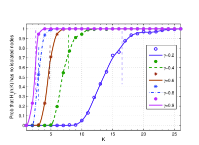
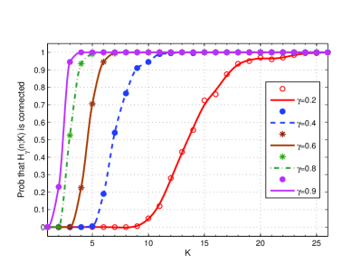
Figure 1: $a)$ Probability that $\mathbb{H}_{\gamma}(n;K)$ contains no isolated for $n=1000$; in each case, the empirical probability value is obtained through $200$ experiments. Vertical dashed lines stand for the critical thresholds asserted by Theorem 11. It is clear that the theoretical findings are in perfect agreement with the practical observations. $b)$ Probability that $\mathbb{H}_{\gamma}(n;K)$ is connected for $n=1,000$ obtained in the same way. Clearly, the curves are almost indistinguishable from the corresponding ones of part $(a)$; this supports the claim that absence of isolated nodes and connectivity are asymptotically equivalent properties.

We also present experimental results that validate Lemma IV.1 and Theorem IV.2: For fixed values of $n$ and $K$ we have constructed key rings according to the mechanism presented in Section II. For each pair of parameters $n$ and $K$, the experiments have been repeated $1,000$ times yielding $1,000\times n$ key rings for each parameter pair. The results are depicted in Figures 1-4 which show the key ring sizes according to their frequency of occurrence. The histograms in blue consider all of the produced $1,000\times n$ key rings, while the histograms in white consider only the $1,000$ maximal key ring sizes, i.e., only the largest key ring among $n$ nodes in an experiment.

It is immediate from Figures 2-3 that the key ring sizes tend to concentrate around $2K$, validating the claim of Lemma IV.1. As would be expected, this concentration becomes more evident as $n$ gets large. It is also clear that, in almost all cases the maximum size of a key ring (out of $n$ nodes) is less than $3K$ validating the claim of Theorem IV.2.

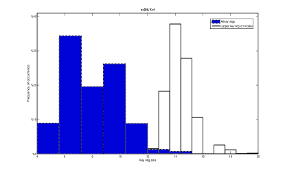
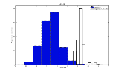
Figure 2: $a)$ Key ring sizes observed in $1,000$ experiments for $n=200$ and $K=4$ – Only 2% of the key rings are larger than $3K$ and the largest key ring has size $20$. $b)$ Key ring sizes observed in $1,000$ experiments for $n=500$ and $K=21$ – Out of the $500,000$ key rings produced only $9$ happened to be larger than $3K$ while the largest size observed is $67$.

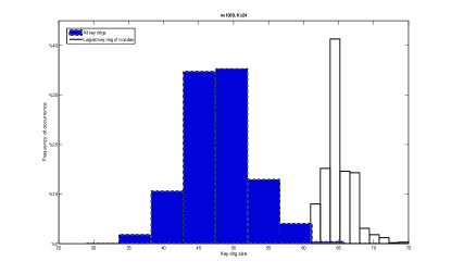
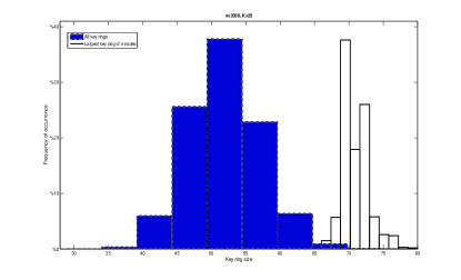
Figure 3: $a)$ Key ring sizes observed in $1,000$ experiments for $n=1,000$ and $K=24$ – $1,000,000$ key rings are produced. Only $5$ of them happened to be larger than $3K$ and the largest observed key ring size is $75$. $b)$ Key ring sizes observed in $1,000$ experiments for $n=2,000$ and $K=26$ – Out of the 2000000 key rings produced only $2$ happened to be larger than $3K$ the largest of them having $80$ keys.

VI Conclusion

In this paper, we consider the pairwise key distribution scheme of Chan et al. which was proposed to establish security in wireless sensor networks. This pairwise scheme has many advantages over other key distribution schemes but deemed not scalable due to $i)$ large number of keys required to establish secure connectivity and $ii)$ the difficulties in the implementation when sensors are required to be deployed in multiple stages. Here, we address this issue and propose an implementation of the pairwise scheme that supports the gradual deployment of sensor nodes in several consecutive phases. We show how should the scheme parameter be adjusted with the number $n$ of sensors so that the secure connectivity can be maintained in the network throughout all stages of the deployment. We also explore the relation between the scheme parameter and the amount of memory that each sensor needs to spare for storing secure keys. By showing that the required number of keys is $O(\log n)$ to achieve connectivity at every step of the deployment, we confirm the scalability of the pairwise scheme in the context of WSNs.

VII A proof of Theorem IV.3

Fix $n=2,3,\ldots$ and $\gamma$ in the interval $(0,1)$, and consider a positive integer $K\geq 2$. Throughout the discussion, $n$ is sufficiently large so that the conditions

$$2(K+1)<n,\quad K+1\leq n-\lfloor\gamma n\rfloor\quad\mbox{and}\quad 2<\gamma n$$ (15)

are all enforced; these conditions are made in order to avoid degenerate situations which have no bearing on the final result. There is no loss of generality in doing so as we eventually let $n$ go to infinity.

For any non-empty subset $R$ contained in $\{1,\ldots,\lfloor\gamma n\rfloor\}$, we define the graph $\mathbb{H}_{\gamma}(n;K)(R)$ (with vertex set $R$) as the subgraph of $\mathbb{H}_{\gamma}(n;K)$ restricted to the nodes in $R$. We say that $R$ is isolated in $\mathbb{H}_{\gamma}(n;K)$ if there are no edges (in $\mathbb{H}_{\gamma}(n;K)$) between the nodes in $R$ and the nodes in its complement $R^{c|\gamma}:=\{1,\ldots,\lfloor\gamma n\rfloor\}-R$. This is characterized by the event $B_{n,\gamma}(K;R)$ given by

$$B_{n,\gamma}(K;R):=\left[i\not\in\Gamma_{n,j},j\notin\Gamma_{n,i},\ i\in R,\ j\in R^{c|\gamma}\right].$$

Also, let $C_{n,\gamma}(K;R)$ denote the event that the induced subgraph $\mathbb{H}_{\gamma}(n;K)(R)$ is itself connected. Finally, we set

$$A_{n,\gamma}(K;R):=C_{n,\gamma}(K;R)\cap B_{n,\gamma}(K;R).$$

The discussion starts with the following basic observation: If $\mathbb{H}_{\gamma}(n;K)$ is not connected, then there must exist a non-empty subset $R$ of nodes contained in $\{1,\ldots,\lfloor\gamma n\rfloor\}$, such that $\mathbb{H}_{\gamma}(n;K)(R)$ is itself connected while $R$ is isolated in $\mathbb{H}_{\gamma}(n;K)$. This is captured by the inclusion

$$C_{n,\gamma}(K)^{c}\subseteq\cup_{R\in\mathcal{N}_{n,\gamma}}~{}A_{n,\gamma}(K;R)$$ (16)

with $\mathcal{N}_{n,\gamma}$ denoting the collection of all non-empty subsets of $\{1,\ldots,\lfloor\gamma n\rfloor\}$. This union need only be taken over all non-empty subsets $R$ of $\{1,\ldots,\lfloor\gamma n\rfloor\}$ with $1\leq|R|\leq\lfloor\frac{\lfloor\gamma n\rfloor}{2}\rfloor$, and it is useful to note that $\lfloor\frac{\lfloor\gamma n\rfloor}{2}\rfloor=\lfloor\frac{\gamma n}{2}\rfloor$. Then, a standard union bound argument immediately gives

$${\mathbb{P}}\left[{C_{n,\gamma}(K)^{c}}\right] \leq \sum_{R\in\mathcal{N}_{n,\gamma}:~{}1\leq|R|\leq\lfloor\frac{\gamma n}{2}\rfloor}{\mathbb{P}}\left[{A_{n,\gamma}(K;R)}\right]$$ (17)

$$= \sum_{r=1}^{\lfloor\frac{\gamma n}{2}\rfloor}\left(\sum_{R\in\mathcal{N}_{n,\gamma,r}}{\mathbb{P}}\left[{A_{n,\gamma}(K;R)}\right]\right)$$

where $\mathcal{N}_{n,\gamma,r}$ denotes the collection of all subsets of $\{1,\ldots,\lfloor\gamma n\rfloor\}$ with exactly $r$ elements.

For each $r=1,\ldots,\lfloor\gamma n\rfloor$, when $R=\{1,\ldots,r\}$, we simplify the notation by writing $A_{n,\gamma,r}(K):=A_{n,\gamma}(K;R)$, $B_{n,\gamma,r}(K):=B_{n,\gamma}(K;R)$ and $C_{n,\gamma,r}(K):=C_{n,\gamma}(K;R)$. For $r=\lfloor\gamma n\rfloor$, the notation $C_{n,\gamma,\lfloor\gamma n\rfloor}(K)$ coincides with $C_{n,\gamma}(K)$ as defined earlier. Under the enforced assumptions, it is a simple matter to check by exchangeability that

$${\mathbb{P}}\left[{A_{n,\gamma}(K;R)}\right]={\mathbb{P}}\left[{A_{n,\gamma,r}(K)}\right],\quad R\in\mathcal{N}_{n.\gamma,r}$$

and the expression

$$\sum_{R\in\mathcal{N}_{\gamma,r}}{\mathbb{P}}\left[{A_{n,\gamma}(K;R)}\right]={\lfloor\gamma n\rfloor\choose r}~{}{\mathbb{P}}\left[{A_{n,\gamma,r}(K)}\right]$$

follows since $|\mathcal{N}_{n,\gamma,r}|={\lfloor\gamma n\rfloor\choose r}$. Substituting into (17) we obtain the bounds

$${\mathbb{P}}\left[{C_{n,\gamma}(K)^{c}}\right]\leq\sum_{r=1}^{\lfloor\frac{\gamma n}{2}\rfloor}{\lfloor\gamma n\rfloor\choose r}~{}{\mathbb{P}}\left[{B_{n,\gamma,r}(K)}\right]$$ (18)

as we make use of the obvious inclusion $A_{n,\gamma,r}(K)\subseteq B_{n,\gamma,r}(K)$. Under the enforced assumptions, we get

$${\mathbb{P}}\left[{B_{n,\gamma,r}(K)}\right]$$

$$= \left({{n-\lfloor\gamma n\rfloor+r-1}\choose K}\over{{n-1}\choose K}\right)^{r}\cdot\left({{n-r-1}\choose K}\over{{n-1}\choose K}\right)^{\lfloor\gamma n\rfloor-r}.$$

To see why this last relation holds, recall that for the set $\{1,\ldots,r\}$ to be isolated in $\mathbb{H}_{\gamma}(n;K)$ we need that (i) each of the nodes $r+1,\ldots,\lfloor\gamma n\rfloor$ are adjacent only to nodes outside the set of nodes $\{1,\ldots,r\}$; and (ii) none of the nodes $1,\ldots,r$ are adjacent with any of the nodes $r+1,\ldots,\lfloor\gamma n\rfloor$ – This last requirement does not preclude adjacency with any of the nodes $\lfloor\gamma n\rfloor+1,\ldots,n$. Reporting (LABEL:eq:ProbCalculation) into (18), we conclude that

$${\mathbb{P}}\left[{C_{n,\gamma}(K)^{c}}\right]$$

$$\leq \sum_{r=1}^{\lfloor\frac{\gamma n}{2}\rfloor}{\lfloor\gamma n\rfloor\choose r}\left({{n-\lfloor\gamma n\rfloor+r-1}\choose K}\over{{n-1}\choose K}\right)^{r}\cdot\left({{n-r-1}\choose K}\over{{n-1}\choose K}\right)^{\lfloor\gamma n\rfloor-r}$$

with conditions (15) ensuring that the binomial coefficients are well defined.

The remainder of the proof consists in bounding each of the terms in (LABEL:eq:BasicIdea+UnionBound3). To do so we make use of several standard bounds. First we recall the well-known bound

$${\lfloor\gamma n\rfloor\choose r}\leq\left(\frac{\lfloor\gamma n\rfloor e}{r}\right)^{r},\quad r=1,\ldots,\lfloor\gamma n\rfloor.$$

Next, for $0\leq K\leq x\leq y$, we note that

$$\frac{{x\choose K}}{{y\choose K}}=\prod_{\ell=0}^{K-1}\left(\frac{x-\ell}{y-\ell}\right)\leq\left(\frac{x}{y}\right)^{K}$$

since $\frac{x-\ell}{y-\ell}$ decreases as $\ell$ increases from $\ell=0$ to $\ell=K-1$.

Now pick $r=1,\ldots,\lfloor\gamma n\rfloor$. Under (15) we can apply these bounds to obtain

$${\lfloor\gamma n\rfloor\choose r}\left({{n-\lfloor\gamma n\rfloor+r-1}\choose K}\over{{n-1}\choose K}\right)^{r}\cdot\left({{n-r-1}\choose K}\over{{n-1}\choose K}\right)^{\lfloor\gamma n\rfloor-r}$$

$$\leq \left(\frac{\lfloor\gamma n\rfloor e}{r}\right)^{r}\cdot\left(\frac{n-\lfloor\gamma n\rfloor+r-1}{n-1}\right)^{rK}$$

$$~{}\times\left(\frac{n-r-1}{n-1}\right)^{K(\lfloor\gamma n\rfloor-r)}$$

$$\leq \left(\frac{\gamma ne}{r}\right)^{r}\left(1-\frac{\lfloor\gamma n\rfloor-r}{n-1}\right)^{rK}\left(1-\frac{r}{n-1}\right)^{K(\lfloor\gamma n\rfloor-r)}$$

$$\leq \left(\gamma ne\right)^{r}\cdot\left(1-\frac{\lfloor\gamma n\rfloor-r}{n}\right)^{rK}\cdot\left(1-\frac{r}{n}\right)^{K(\lfloor\gamma n\rfloor-r)}$$

$$\leq \left(\gamma ne\right)^{r}\cdot e^{-\left(\frac{\lfloor\gamma n\rfloor-r}{n}\right)rK}\cdot e^{-\left(\frac{r}{n}\right)(\lfloor\gamma n\rfloor-r)K}.$$

It is plain that

$${\mathbb{P}}\left[{C_{n,\gamma}(K)^{c}}\right] \leq \sum_{r=1}^{\lfloor\frac{\gamma n}{2}\rfloor}\left(\gamma ne\right)^{r}\cdot e^{-2\left(\frac{\lfloor\gamma n\rfloor-r}{n}\right)rK}$$ (21)

$$\leq \sum_{r=1}^{\lfloor\frac{\gamma n}{2}\rfloor}\left(\gamma ne\cdot e^{-2\left(\frac{\lfloor\gamma n\rfloor-\lfloor\frac{\gamma n}{2}\rfloor}{n}\right)K}\right)^{r}$$

as we note that

$$\frac{\lfloor\gamma n\rfloor-r}{n}\geq\frac{\lfloor\gamma n\rfloor-\lfloor\frac{\gamma n}{2}\rfloor}{n},\quad r=1,\ldots,\lfloor\frac{\gamma n}{2}\rfloor.$$

Next, consider a scaling $K:\mathbb{N}_{0}\rightarrow\mathbb{N}_{0}$ such that (9) holds for some $c>1$, and replace $K$ by $K_{n}$ in (21) according to this scaling. Using the form (9) of the scaling we get,

$$a_{n}:=\gamma ne\cdot e^{-2\left(\frac{\lfloor\gamma n\rfloor-\lfloor\frac{\gamma n}{2}\rfloor}{n}\right)K_{n}}=(\gamma e)\cdot n^{1-2c_{n}\left(\frac{\lfloor\gamma n\rfloor-\lfloor\frac{\gamma n}{2}\rfloor}{\gamma n}\right)}$$

for each $n=1,2,\ldots$, with $\lim_{n\rightarrow\infty}c_{n}=c$. It is a simple matter to check that

$$\lim_{n\rightarrow\infty}\left(2c_{n}\left(\frac{\lfloor\gamma n\rfloor-\lfloor\frac{\gamma n}{2}\rfloor}{\gamma n}\right)\right)=c,$$

so that by virtue of the fact that $c>1$, we have

$$\lim_{n\rightarrow\infty}a_{n}=0.$$ (22)

From (21) we conclude that

$${\mathbb{P}}\left[{C_{n,\gamma}(K_{n})^{c}}\right]\leq\sum_{r=1}^{\lfloor\frac{\gamma n}{2}\rfloor}\left(a_{n}\right)^{r}\leq\sum_{r=1}^{\infty}\left(a_{n}\right)^{r}=\frac{a_{n}}{1-a_{n}}$$

where for $n$ sufficiently large the summability of the geometric series is guaranteed by (22). The conclusion $\lim_{n\to\infty}{\mathbb{P}}\left[{C_{n,\gamma}(K)^{c}}\right]=0$ is now a straightforward consequence of the last bound, again by virtue of (22).

VIII A proof of Theorem 11

Fix $n=2,3,\ldots$ and consider $\gamma$ in $(0,1)$ and positive integer $K$ such that $K<n$. We write

$$\chi_{n,\gamma,i}(K):={\bf 1}\left[{\rm Node~{}}i~{}{\rm is~{}isolated~{}in~{}}\mathbb{H}_{\gamma}(n;K)\right]$$

for each $i=1,\ldots,\lfloor\gamma n\rfloor$. The number of isolated nodes in $\mathbb{H}_{\gamma}(n;K)$ is simply given by

$$I_{n,\gamma}(K):=\sum_{i=1}^{\lfloor\gamma n\rfloor}\chi_{n,\gamma,i}(K),$$

whence the random graph $\mathbb{H}_{\gamma}(n;K)$ has no isolated nodes if $I_{n,\gamma}(K)=0$. The method of first moment [8, Eqn (3.10), p. 55] and second moment [8, Remark 3.1, p. 55] yield the useful bounds

$$1-{\mathbb{E}}\left[{I_{n,\gamma}(K)}\right]\leq{\mathbb{P}}\left[{I_{n,\gamma}(K)=0}\right]\leq 1-\frac{{\mathbb{E}}\left[{I_{n,\gamma}(K)}\right]^{2}}{{\mathbb{E}}\left[{I_{n,\gamma}(K)^{2}}\right]}.$$ (23)

The rvs $\chi_{n,\gamma,1}(K),\ldots,\chi_{n,\gamma,\lfloor\gamma n\rfloor}(K)$ being exchangeable, we find

$${\mathbb{E}}\left[{I_{n,\gamma}(K)}\right]=\lfloor\gamma n\rfloor{\mathbb{E}}\left[{\chi_{n,\gamma,1}(K)}\right]$$ (24)

and

$${\mathbb{E}}\left[{I_{n,\gamma}(K)^{2}}\right]$$

$$= \lfloor\gamma n\rfloor{\mathbb{E}}\left[{\chi_{n,\gamma,1}(K)}\right]$$

$$~{}+\lfloor\gamma n\rfloor(\lfloor\gamma n\rfloor-1){\mathbb{E}}\left[{\chi_{n,\gamma,1}(K)\chi_{n,\gamma,2}(K)}\right]$$

by the binary nature of the rvs involved. It then follows in the usual manner that

$$\frac{{\mathbb{E}}\left[{I_{n,\gamma}(K)^{2}}\right]}{{\mathbb{E}}\left[{I_{n,\gamma}(K)}\right]^{2}} = \frac{1}{\lfloor\gamma n\rfloor{\mathbb{E}}\left[{\chi_{n,\gamma,1}(K)}\right]}$$

$$~{}+\frac{\lfloor\gamma n\rfloor-1}{\lfloor\gamma n\rfloor}\frac{{\mathbb{E}}\left[{\chi_{n,\gamma,1}(K)\chi_{n,\gamma,2}(K)}\right]}{\left({\mathbb{E}}\left[{\chi_{n,\gamma,1}(K)}\right]\right)^{2}}.$$

From (23) and (24) we conclude that the one-law $\lim_{n\to\infty}{\mathbb{P}}\left[{I_{n,\gamma}(K_{n})=0}\right]=1$ holds if we show that

$$\lim_{n\to\infty}\lfloor\gamma n\rfloor{\mathbb{E}}\left[{\chi_{n,\gamma,1}(K_{n})}\right]=0.$$ (27)

On the other hand, it is plain from (23) and (VIII) that the zero-law $\lim_{n\to\infty}{\mathbb{P}}\left[{I_{n,\gamma}(K_{n})=0}\right]=0$ will be established if

$$\lim_{n\to\infty}\lfloor\gamma n\rfloor{\mathbb{E}}\left[{\chi_{n,1}(K_{n})}\right]=\infty$$ (28)

and

$$\limsup_{n\to\infty}\left(\frac{{\mathbb{E}}\left[{\chi_{n,\gamma,1}(K_{n})\chi_{n,\gamma,2}(K_{n})}\right]}{\left({\mathbb{E}}\left[{\chi_{n,\gamma,1}(K_{n})}\right]\right)^{2}}\right)\leq 1.$$ (29)

The next two technical lemmas establish (27), (28) and (29) under the appropriate conditions on the scaling $K:\mathbb{N}_{0}\rightarrow\mathbb{N}_{0}$.

Lemma VIII.1

Consider $\gamma$ in $(0,1)$ and a scaling $K:\mathbb{N}_{0}\rightarrow\mathbb{N}_{0}$ such that (9) holds for some $c>0$. We have

$$\lim_{n\rightarrow\infty}n{\mathbb{E}}\left[{\chi_{n,\gamma,1}(K_{n})}\right]=\left\{\begin{array}[]{ll}0&\mbox{if~{} $c>r(\gamma)$}\\ &\\ \infty&\mbox{if~{}$c<r(\gamma)$}\end{array}\right.$$ (30)

with $r(\gamma)$ specified via (11).

Lemma VIII.2

Consider $\gamma$ in $(0,1)$ and a scaling $K:\mathbb{N}_{0}\rightarrow\mathbb{N}_{0}$ such that (9) holds for some $c>0$. We have

$$\limsup_{n\to\infty}\left(\frac{{\mathbb{E}}\left[{\chi_{n,\gamma,1}(K_{n})\chi_{n,\gamma,2}(K_{n})}\right]}{\left({\mathbb{E}}\left[{\chi_{n,\gamma,1}(K_{n})}\right]\right)^{2}}\right)\leq 1.$$ (31)

Proofs of Lemma VIII.1 and Lemma 31 can be found in Section VIII-A and Section VIII-B, respectively. To complete the proof of Theorem 11, pick a scaling $K:\mathbb{N}_{0}\rightarrow\mathbb{N}_{0}$ such that (9) holds for some $c>0$. Under the condition $c>r(\gamma)$ we get (27) from Lemma VIII.1 and the one-law $\lim_{n\to\infty}{\mathbb{P}}\left[{I_{n,\gamma}(K_{n})=0}\right]=1$ follows. Next, assume the condition $c<r(\gamma)$. We obtain (28) and (29) with the help of Lemmas VIII.1 and 31, respectively, and the conclusion $\lim_{n\to\infty}{\mathbb{P}}\left[{I_{n,\gamma}(K_{n})=0}\right]=0$ is now immediate.

VIII-A A proof of Lemma VIII.1

Fix $n=2,3,\ldots$ and $\gamma$ in $(0,1)$, and consider a positive integer $K$ such that $K<n$. Here as well there is no loss of generality in assuming $n-\lfloor\gamma n\rfloor\geq K$ and $\lfloor\gamma n\rfloor>1$. Under the enforced assumptions, we get

$${\mathbb{E}}\left[{\chi_{n,\gamma,1}(K)}\right] = \frac{{n-\lfloor\gamma n\rfloor\choose K}}{{n-1\choose K}}\left(\frac{{n-2\choose K}}{{n-1\choose K}}\right)^{\lfloor\gamma n\rfloor-1}$$ (32)

$$= a(n;K)\cdot\left(1-\frac{K}{n-1}\right)^{\lfloor\gamma n\rfloor-1}$$

with

$$a(n;K):=\frac{(n-\lfloor\gamma n\rfloor)!}{(n-\lfloor\gamma n\rfloor-K)!}\cdot\frac{(n-1-K)!}{(n-1)!}.$$

Now pick a scaling $K:\mathbb{N}_{0}\rightarrow\mathbb{N}_{0}$ such that (9) holds for some $c>0$ and replace $K$ by $K_{n}$ in (32) with respect to this scaling. Applying Stirling’s formula

$$m!\sim\sqrt{2\pi m}\left(\frac{m}{e}\right)^{m}\quad(m\rightarrow\infty)$$

to the factorials appearing in (32), we readily get

$$a(n;K_{n}) \sim \sqrt{\frac{(n-\lfloor\gamma n\rfloor)(n-1-K_{n})}{(n-\lfloor\gamma n\rfloor-K_{n})(n-1)}}\cdot\alpha_{n}\beta_{n}$$ (33)

$$\sim \alpha_{n}\beta_{n}$$

under the enforced assumptions on the scaling with

$$\alpha_{n} := \frac{(n-K_{n}-1)^{n-K_{n}-1}}{(n-1)^{n-1}}$$

$$= \left(1-\frac{K_{n}}{n-1}\right)^{n-1}\cdot\left(n-K_{n}-1\right)^{-K_{n}}$$

and

$$\beta_{n} := \frac{(n-\lfloor\gamma n\rfloor)^{n-\lfloor\gamma n\rfloor}}{(n-\lfloor\gamma n\rfloor-K_{n})^{n-\lfloor\gamma n\rfloor-K_{n}}}$$

$$= \left(1-\frac{K_{n}}{n-\lfloor\gamma n\rfloor}\right)^{-(n-\lfloor\gamma n\rfloor)}\cdot\left(n-\lfloor\gamma n\rfloor-K_{n}\right)^{K_{n}}.$$

In obtaining the asymptotic behavior of (33) we rely on the following technical fact: For any sequence $m:\mathbb{N}_{0}\rightarrow\mathbb{N}_{0}$ with $m_{n}=O(n)$, we have

$$\left(1-\frac{K_{n}}{m_{n}}\right)^{m_{n}}\sim e^{-K_{n}}.$$ (34)

To see why (34) holds, recall the elementary decomposition

$$\log(1-x)=-x-\Psi(x)\ \mbox{with}\quad\Psi(x):=\int_{0}^{x}\frac{t}{1-t}~{}dt$$

valid for $0\leq x<1$. Using this fact, we get

$$\left(1-\frac{K_{n}}{m_{n}}\right)^{m_{n}}=e^{-K_{n}}\cdot e^{-m_{n}\Psi\left(\frac{K_{n}}{m_{n}}\right)}$$ (35)

for all $n=1,2,\ldots$.

Under the enforced assumptions we have $m_{n}=O(n)$ and $K_{n}=O(\log n)$, so that

$$\lim_{n\rightarrow\infty}\frac{K_{n}}{m_{n}}=0\quad\mbox{and}\quad\lim_{n\rightarrow\infty}m_{n}\left(\frac{K_{n}}{m_{n}}\right)^{2}=0.$$

It is now plain that

$$\lim_{n\rightarrow\infty}m_{n}\Psi\left(\frac{K_{n}}{m_{n}}\right)=0$$

as we note that $\lim_{x\downarrow 0}\frac{\Psi(x)}{x^{2}}=\frac{1}{2}$. This establishes (34) via (35).

Using (34), first with $m_{n}=n-1$, then with $m_{n}=n-\lfloor\gamma n\rfloor$, we obtain

$$\left(1-\frac{K_{n}}{n-1}\right)^{n-1}\sim e^{-K_{n}}$$

and

$$\left(1-\frac{K_{n}}{n-\lfloor\gamma n\rfloor}\right)^{-(n-\lfloor\gamma n\rfloor)}\sim\left(e^{-K_{n}}\right)^{-1}=e^{K_{n}},$$

whence

$$\alpha_{n}\beta_{n}\sim\left(\frac{n-\lfloor\gamma n\rfloor-K_{n}}{n-K_{n}-1}\right)^{K_{n}}.$$ (36)

With the help of (32) and (33) we now conclude that

$$n{\mathbb{E}}\left[{\chi_{n,\gamma,1}(K_{n})}\right]$$

$$\sim n\left(1-\frac{K_{n}}{n-1}\right)^{\lfloor\gamma n\rfloor-1}\cdot\left(\frac{n-\lfloor\gamma n\rfloor-K_{n}}{n-K_{n}-1}\right)^{K_{n}}.$$

A final application of (34), this time with $m_{n}=n-1$, gives

$$\left(1-\frac{K_{n}}{n-1}\right)^{\lfloor\gamma n\rfloor-1} = \left(\left(1-\frac{K_{n}}{n-1}\right)^{n-1}\right)^{\frac{\lfloor\gamma n\rfloor-1}{n-1}}$$ (38)

$$\sim e^{-\frac{\lfloor\gamma n\rfloor-1}{n-1}K_{n}}$$

since $\lim_{n\rightarrow\infty}\frac{\lfloor\gamma n\rfloor-1}{n-1}=\gamma$. Reporting (38) into (LABEL:eq:Intermediary1) we obtain

$$n{\mathbb{E}}\left[{\chi_{n,\gamma,1}(K_{n})}\right]\sim e^{\zeta_{n}}$$ (39)

with

$$\zeta_{n}:=\log n-\left(\frac{\lfloor\gamma n\rfloor-1}{n-1}+\log\left(\frac{n-\lfloor\gamma n\rfloor-K_{n}}{n-K_{n}-1}\right)\right)K_{n}$$

for all $n=1,2,\ldots$. Finally, from the condition (9) on the scaling, we see that

$$\lim_{n\rightarrow\infty}\frac{\zeta_{n}}{\log n}=1-c+c\frac{\log(1-\gamma)}{\gamma}=1-\frac{c}{r(\gamma)}.$$

Thus, $\lim_{n\rightarrow\infty}\zeta_{n}=-\infty$ (resp. $\infty$) if $r(\gamma)>c$ (resp. $r(\gamma)<c$) and the desired result follows upon using (39).

VIII-B A proof of Lemma 31

Fix positive integers $n=3,4,\ldots$ and $K$ with $K<n$. With $\gamma$ in $(0,1)$, we again assume that $n-\lfloor\gamma n\rfloor\geq K$ and $\lfloor\gamma n\rfloor>1$. It is a simple matter to check that

$${\mathbb{E}}\left[{\chi_{n,\gamma,1}(K)\chi_{n,\gamma,2}(K)}\right]=\left({{n-\lfloor\gamma n\rfloor}\choose{K}}\over{{n-1}\choose{K}}\right)^{2}\left({{n-3}\choose{K}}\over{{n-1}\choose{K}}\right)^{\lfloor\gamma n\rfloor-2}$$

and invoking (32) we readily conclude that

$$\frac{{\mathbb{E}}\left[{\chi_{n,\gamma,1}(K)\chi_{n,\gamma,2}(K)}\right]}{\left({\mathbb{E}}\left[{\chi_{n,\gamma,1}(K)}\right]\right)^{2}}$$ (40)

$$= \left({{n-3}\choose{K}}\over{{n-1}\choose{K}}\right)^{\lfloor\gamma n\rfloor-2}\cdot\left(\frac{{n-1\choose K}}{{n-2\choose K}}\right)^{2\left(\lfloor\gamma n\rfloor-1\right)}$$

$$= \left(\left(\frac{n-1-K}{n-1}\right)\left(\frac{n-2-K}{n-2}\right)\right)^{\lfloor\gamma n\rfloor-2}$$

$$~{}\times\left(\frac{n-1}{n-1-K}\right)^{2\left(\lfloor\gamma n\rfloor-1\right)}$$

$$= \left(\frac{n-2-K}{n-2}\right)^{\lfloor\gamma n\rfloor-2}\cdot\left(\frac{n-1}{n-1-K}\right)^{\lfloor\gamma n\rfloor}$$

$$= \left(1-\frac{K}{n-2}\right)^{\lfloor\gamma n\rfloor-2}\cdot\left(1+\frac{K}{n-1-K}\right)^{\lfloor\gamma n\rfloor}$$

$$\leq e^{-K\cdot E(n;K)}$$

where we have set

$$E(n;K):=\frac{\lfloor\gamma n\rfloor-2}{n-2}-\frac{\lfloor\gamma n\rfloor}{n-1-K}.$$

Elementary calculations show that

$$-K\cdot E(n;K)=\frac{\lfloor\gamma n\rfloor}{n-2}\cdot\frac{K(K-1)}{n-1-K}+\frac{2K}{n-2}.$$

Now pick a scaling $K:\mathbb{N}_{0}\rightarrow\mathbb{N}_{0}$ such that (9) holds for some $c>0$. It is plain that $\lim_{n\rightarrow\infty}K_{n}E(n;K_{n})=0$ and the conclusion (31) follows from (40).

IX A proof of Theorem 14

Pick $0<\gamma_{1}<\gamma_{2}<\ldots<\gamma_{\ell}\leq 1$ and consider a scaling $K:\mathbb{N}_{0}\rightarrow\mathbb{N}_{0}$ such that

$$K_{n}\sim c~{}\frac{\log n}{\gamma_{1}}$$

for some $c>1$. It is plain that (14) will hold provided

$$\lim_{n\to\infty}{\mathbb{P}}\left[{C_{n,\gamma_{k}}(K_{n})}\right]=1,\quad k=1,\ldots,\ell.$$ (41)

For each $k=1,2,\ldots,\ell$, we note that

$$c~{}\frac{\log n}{\gamma_{1}}=c_{k}~{}\frac{\log n}{\gamma_{k}}\quad\mbox{with~{}}c_{k}:=c~{}\frac{\gamma_{k}}{\gamma_{1}}$$

for all $n=1,2,\ldots$. But $c>1$ implies $c_{k}>1$ since $\gamma_{1}<\ldots<\gamma_{\ell}$. As a result, $\mathbb{H}_{\gamma_{k}}(n;K_{n})$ will be a.a.s. connected by virtue of Theorem IV.3 applied to $\mathbb{H}_{\gamma_{k}}(n;K)$, and (41) indeed holds.

X A proof of Lemma IV.1

Fix $n=2,3,\ldots$ and positive integer $K$ with $K<n$. For each $i=1,2,\ldots,n$, node $i$ is assigned a key ring $\Sigma_{n,i}$ whose size is given by

$$|\Sigma_{n,i}|=|\Gamma_{n,i}|+\sum_{j=1,\ j\neq i}^{n}{\bf 1}\left[i\in\Gamma_{n,j}\right].$$ (42)

This is a simple consequence of the definition (1). We also define the maximal key ring size as

$$M_{n}:={\max}_{i=1,\ldots,n}|\Sigma_{n,i}|.$$

It is easy to see that

$$|\Sigma_{n,i}|=K+B_{n,i}$$ (43)

where $B_{n,i}$ is the rv determined through

$$B_{n,i}:=\sum_{j=1,\ j\neq i}^{n}{\bf 1}\left[i\in\Gamma_{n,j}\right].$$

Under the enforced independence assumptions, the rv $B_{n,i}$ is a binomial rv ${\rm Bin}(n-1,\frac{K}{n-1})$, with

$${\mathbb{E}}\left[{B_{n,i}}\right]=(n-1)\cdot\frac{K}{n-1}=K$$

and

$${\rm Var}[B_{n,i}]=(n-1)\cdot\frac{K}{n-1}\cdot\frac{n-1-K}{n-1}.$$

As a result, ${\mathbb{E}}\left[{|\Sigma_{n,i}|}\right]=2K$ and

$${\rm Var}[|\Sigma_{n,i}|]=K\left(1-\frac{K}{n-1}\right).$$

It is now plain that

$${\mathbb{E}}\left[{\left|\frac{|\Sigma_{n,i}|}{{\mathbb{E}}\left[{|\Sigma_{n,i}|}\right]}-1\right|^{2}}\right] = \frac{{\rm Var}[|\Sigma_{n,i}|]}{{\mathbb{E}}\left[{|\Sigma_{n,i}|}\right]^{2}}$$ (44)

$$= \frac{1}{4}\left(\frac{1}{K}-\frac{1}{n-1}\right)$$

so that

$${\mathbb{E}}\left[{\left|\frac{|\Sigma_{n,i}|}{2K}-1\right|^{2}}\right]=\frac{1}{4}\left(\frac{1}{K}-\frac{1}{n-1}\right).$$ (45)

Under the enforced assumptions, we have

$$\lim_{n\rightarrow\infty}{\mathbb{E}}\left[{\left|\frac{|\Sigma_{n,1}(K_{n})|}{2K_{n}}-1\right|^{2}}\right]=0$$

by the earlier calculations (45), and the desired result (5) follows.  

XI A proof of Theorem IV.2

Fix the positive integers $n=2,3,\ldots$ and $K$ with $K<n$. Using (43) we readily get

$$\left(\max_{i=1,\ldots,n}|\Sigma_{n,i}|\right)-2K=\max_{i=1,\ldots,n}\left(B_{n,i}-K\right).$$

Therefore, with any given $t>0$, we find

$${\mathbb{P}}\left[{\left|\left(\max_{i=1,\ldots,n}|\Sigma_{n,i}|\right)-2K\right|>t}\right]$$ (46)

$$= {\mathbb{P}}\left[{\left|\max_{i=1,\ldots,n}\left(B_{n,i}-K\right)\right|>t}\right]$$

$$= {\mathbb{P}}\left[{\max_{i=1,\ldots,n}B_{n,i}>K+t}\right]$$

$$~{}+{\mathbb{P}}\left[{\max_{i=1,\ldots,n}B_{n,i}<K-t}\right].$$

We take each term in turn. First a simple union argument shows that

$${\mathbb{P}}\left[{{\max}_{i=1,\ldots,n}B_{n,i}>K+t}\right]$$ (47)

$$= {\mathbb{P}}\left[{\cup_{i=1}^{n}[B_{n,i}>K+t]}\right]$$

$$\leq \sum_{i=1}^{n}{\mathbb{P}}\left[{B_{n,i}>K+t}\right]$$

$$= n{\mathbb{P}}\left[{B_{n,1}>K+t}\right]$$

since the rvs $B_{n,1},\ldots,B_{n,n}$ are identically distributed (but not independent). Next we note that

$${\mathbb{P}}\left[{{\max}_{i=1,\ldots,n}B_{n,i}<K-t}\right]$$ (48)

$$= {\mathbb{P}}\left[{B_{n,i}<K-t,\ i=1,\ldots n}\right]$$

$$\leq {\min}_{i=1,\ldots,n}{\mathbb{P}}\left[{B_{n,i}<K-t}\right]$$

$$= {\mathbb{P}}\left[{B_{n,1}<K_{n}-t}\right].$$

To proceed we recall standard bounds for the tails of binomial rvs [9, lemma 1.1, p. 16]: With

$$H(t):=1-t+t\log t,$$

we have the concentration inequalities

$${\mathbb{P}}\left[{B_{n.1}>K+t}\right]\leq e^{-K\cdot H(\frac{K+t}{K})}$$

and

$${\mathbb{P}}\left[{B_{n,1}<K-t}\right]\leq e^{-K\cdot H(\frac{K-t}{K})}$$

where the additional condition $0<t<K$ is required for the second inequality to hold. Simple calculations on the appropriate ranges show that

$$-K\cdot H\left(\frac{K\pm t}{K}\right)=\pm t-\left(K\pm t\right)\cdot\log\left(1\pm\frac{t}{K}\right).$$

Thus, by the first concentration inequality, we conclude from (47) that

$${\mathbb{P}}\left[{{\max}_{i=1,\ldots,n}B_{n,i}>K+t}\right]\leq e^{A_{n}(K;t)}$$ (49)

with

$$A_{n}(K;t):=\log n+t-\left(K+t\right)\cdot\log\left(1+\frac{t}{K}\right).$$

The second concentration inequality and (48) together yield

$${\mathbb{P}}\left[{{\max}_{i=1,\ldots,n}B_{n,i}<K-t}\right]\leq e^{B_{n}(K;t)}$$ (50)

with

$$B_{n}(K;t):=-t-\left(K-t\right)\cdot\log\left(1-\frac{t}{K}\right)$$

under the additional constraint $0<t<K$.

Now consider a scaling $K:\mathbb{N}_{0}\rightarrow\mathbb{N}_{0}$ of the form (6) for some $\gamma>0$, and select the sequence $t:\mathbb{N}_{0}\rightarrow\mathbb{R}_{+}$ given by

$$t_{n}=clogn,\quad n=1,2,\ldots$$

with $c$ in the interval $(0,\gamma)$ (so that $0<t_{n}<K_{n}$ for all $n$ sufficiently large).

Under appropriate conditions on $\gamma$ and $c$, we shall show that

$$\lim_{n\rightarrow\infty}A_{n}(K_{n};t_{n})=-\infty$$ (51)

and

$$\lim_{n\rightarrow\infty}B_{n}(K_{n};t_{n})=-\infty.$$ (52)

The convergence statements

$$\lim_{n\rightarrow\infty}{\mathbb{P}}\left[{{\max}_{i=1,\ldots,n}B_{n,i}(K_{n})>K_{n}+t_{n}}\right]=0$$

and

$$\lim_{n\rightarrow\infty}{\mathbb{P}}\left[{{\max}_{i=1,\ldots,n}B_{n,i}(K_{n})<K_{n}-t_{n}}\right]=0$$

then follow from (49) and (50), respectively, and the desired conclusion (7) flows from (46).

With the selections made above, we get $A_{n}(K_{n};t_{n})\sim a(\gamma;c)\log n$ and $B_{n}(K_{n};t_{n})\sim b(\gamma;c)\log n$ with coefficients $a(\gamma;c)$ and $b(\gamma;c)$ given by

$$a(\gamma;c):=1+c-\left(\gamma+c\right)\cdot\log\left(1+\frac{c}{\gamma}\right),\quad c>0$$

and

$$b(\gamma;c):=-c-\left(\gamma-c\right)\cdot\log\left(1-\frac{c}{\gamma}\right),\quad 0<c<\gamma.$$

Thus, in order to ensure (51) and (52), we need to find $c$ in the interval $(0,\gamma)$ such that $a(\gamma;c)<0$ and $b(\gamma;c)<0$, respectively. To that end, we first note that

$$\frac{\partial a}{\partial c}(\gamma;c)=-\log\left(1+\frac{c}{\gamma}\right)<0,\quad c>0$$

and

$$\frac{\partial b}{\partial c}(\gamma;c)=\log\left(1-\frac{c}{\gamma}\right)<0,\quad 0<c<\gamma.$$

Therefore, both mappings $c\rightarrow a(\gamma;c)$ and $c\rightarrow b(\gamma;c)$ are strictly decreasing on the intervals $(0,\infty)$ and $(0,\gamma)$, respectively. Since $\lim_{c\downarrow 0}b(\gamma;c)=0$, it is plain that $b(\gamma;c)<0$ on the entire interval $(0,\gamma)$. On the other hand, it is easy to check that $\lim_{c\downarrow 0}a(\gamma;c)=1$ and

$$\lim_{c\uparrow\gamma}a(\gamma;c)=1-\gamma\left(2\log 2-1\right)=1-\frac{\gamma}{\gamma^{\star}}.$$

Hence, if we select $\gamma>\gamma^{\star}$, then $a(\gamma;c)<0$ for all $c>c(\gamma)$ where $c(\gamma)$ is the unique solution to the equation

$$a(\gamma;c)=0,\quad c>0.$$ (53)

Uniqueness is a consequence of the strict monotonicity mentioned earlier.

The proof will be completed by showing that the constraint

$$c(\gamma)<\gamma,\quad\gamma>\gamma^{\star}$$ (54)

indeed holds. For each $\gamma>0$, define the quantity $x(\gamma):=\frac{c(\gamma)}{\gamma}$. In view of (53) it is the unique solution to the equation

$$\frac{1}{\gamma}+x-(1+x)\log\left(1+x\right)=0,\quad x>0.$$ (55)

This equation is equivalent to

$$\frac{1}{\gamma}=\varphi(x),\quad x>0$$ (56)

where the mapping $\varphi:\mathbb{R}_{+}\rightarrow\mathbb{R}_{+}$ is given by

$$\varphi(x)=(1+x)\log\left(1+x\right)-x,\quad x\geq 0.$$

This mapping $\varphi:\mathbb{R}_{+}\rightarrow\mathbb{R}_{+}$ is strictly monotone increasing with $\lim_{x\downarrow 0}\varphi(x)=0$ and $\lim_{x\uparrow\infty}\varphi(x)=\infty$, so that $\varphi$ is a bijection from $\mathbb{R}_{+}$ onto itself. It then follows from (56) that $x(\gamma)$ is strictly decreasing as $\gamma$ increases. Since $\varphi(1)=\left(\gamma^{\star}\right)^{-1}$, we get $x(\gamma^{\star})=1$ by uniqueness, whence $x(\gamma)<x(\gamma^{\star})=1$ for $\gamma>\gamma^{\star}$, a statement equivalent to (54).

Careful inspection of the proof shows that (8) holds with

$$h(\gamma;c):=-\max\left(a(\gamma;c),b(\gamma;c)\right)$$ (57)

on the range $c(\gamma)<c<\gamma$, and it is clear from the discussion above that $h(\gamma;c)>0$ when $\gamma>\gamma^{\star}$.

References

• [1] S.R. Blackburn and S. Gerke, β€œConnectivity of the uniform random intersection graph,” Discrete Mathematics 309 (2009), pp. 5130-5140.
• [2] B. BollobΓ‘s, Random Graphs, Second Edition, Cambridge Studies in Advanced Mathematics, Cambridge University Press, Cambridge (UK), 2001.
• [3] H. Chan, A. Perrig and D. Song, β€œRandom key predistribution schemes for sensor networks,” in Proceedings of the SP 2003, Oakland (CA), May 2003, pp. 197-213.
• [4] R. Di Pietro, L.V. Mancini, A. Mei, A. Panconesi and J. Radhakrishnan, β€œRedoubtable sensor networks,” ACM Transactions on Information Systems Security TISSEC 11 (2008), pp. 1-22.
• [5] W. Du, J. Deng, Y.S. Han and P.K. Varshney, β€œA pairwise key pre-distribution scheme for wireless sensor networks,” in Proceedings of the CCS 2003, Washington (DC), October 2004.
• [6] L. Eschenauer and V.D. Gligor, β€œA key-management scheme for distributed sensor networks,” in Proceedings of the CSS 2002, Washington (DC), November 2002, pp. 41-47.
• [7] J. Hwang and Y. Kim, β€œRevisiting random key pre-distribution schemes for wireless sensor networks,” in Proceedings of the SASN 2004, Washington (DC), October 2004.
• [8] S. Janson, T. Łuczak and A. RuciΕ„ski, Random Graphs, Wiley-Interscience Series in Discrete Mathematics and Optimization, John Wiley & Sons, 2000.
• [9] M.D. Penrose, Random Geometric Graphs, Oxford Studies in Probability 5, Oxford University Press, New York (NY), 2003.
• [10] A. Perrig, J. Stankovic and D. Wagner, β€œSecurity in wireless sensor networks,” Communications of the ACM 47 (2004), pp. 53–57.
• [11] K. Rybarczyk β€œDiameter, connectivity and phase transition of the uniform random intersection graph,” Submitted to Discrete Mathematics, July 2009.
• [12] D.-M. Sun and B. He, β€œReview of key management mechanisms in wireless sensor networks,” Acta Automatica Sinica 12 (2006), pp. 900-906.
• [13] O. Yağan and A.M. Makowski, β€œOn the random graph induced by a random key predistribution scheme under full visibility,” in Proceedings of the ISIT 2008, Toronto (ON), June 2008.
• [14] O. Yağan and A. M. Makowski, β€œConnectivity results for random key graphs,” in Proceedings of the ISIT 2009, Seoul (Korea), June 2009.
• [15] O. Yağan and A.M. Makowski, β€œZero-one laws for connectivity in random key graphs,” Available online at arXiv:0908.3644v1 [math.CO], August 2009.
• [16] O. Yağan and A. M. Makowski, β€œOn random pairwise graphs,” to be submitted to Discrete Mathematics. Available online at http://www.ece.umd.edu/~oyagan/Journals/Pairwise-DM.pdf