Radiation feedback on dusty clouds during Seyfert activity

Abstract

We investigate the evolution of dusty gas clouds falling into the centre of an active Seyfert nucleus. Two-dimensional high-resolution radiation hydrodynamics simulations are performed to study the fate of single clouds and the interaction between two clouds approaching the Active Galactic Nucleus. We find three distinct phases of the evolution of the cloud: (i) formation of a lenticular shape with dense inner rim caused by the interaction of gravity and radiation pressure (the lense phase), (ii) formation of a clumpy sickle-shaped structure as the result of a converging flow (the clumpy sickle phase) and (iii) a filamentary phase caused by a rapidly varying optical depth along the sickle. Depending on the column density of the cloud, it will either be pushed outwards or its central (highest column density) parts move inwards, while there is always some material pushed outwards by radiation pressure effects. The general dynamical evolution of the cloud can approximately be described by a simple analytical model.

1 Introduction

Normal spiral galaxies light up as soon as enough gas is accreted onto their nuclei. Then, their central region becomes similarly bright as the stars of the whole galaxy, a phenomenon called Seyfert activity (Seyfert, 1943; Weedman, 1977; Sanders, 1981). It is thought that this is a recurrent process and most of the normal galaxies have encountered such activity cycles during the growth phase of their central supermassive black holes, whenever enough gas reaches their centres. A fast rotating, thin and hot gaseous accretion disc forms, which is surrounded by a ring-like, dusty, geometrically thick gas reservoir – the so-called dusty torus. Anisotropically blocking the light, this gives rise to two characteristic observational signatures, depending whether the line of sight is obscured (edge-on view, so-called Seyfert 2 galaxies) or not (face-on view, so-called Seyfert 1 galaxies). These nuclear regions of nearby Seyfert galaxies, as well as our own galactic centre have been observed in great detail with the most up-to-date instruments at the largest available telescopes and interferometers, yielding unprecedented resolution (e. g.  Davies et al., 2007; Tristram et al., 2007; Tristram et al., 2009; Burtscher et al., 2009; Prieto et al., 2010; Hönig et al., 2010). Therefore, they represent an ideal testbed for studying fueling processes and the characteristics of active galactic nuclei (AGN). Only a few models capable of explaining the necessary fueling process have been presented up to today. For example Elitzur & Shlosman (2006) argue for fueling of the central region through a midplane influx of cold and clumpy material from the galaxy (Shlosman et al., 1990). When reaching the centre, the gas will contribute to the formation of a hot accretion disc that illuminates the surrounding region. A hydromagnetically or radiatively driven disc wind forms. The embedded dusty and optically thick clouds then form the Toroidal Obscuration Region (TOR) in the parsec scale vicinity of the central engine, which replaces the classical torus in their model. The accretion process from galactic scales down to sub-parsec scales has also been followed in great detail by Hopkins & Quataert (2010) in multiscale SPH (smoothed particle hydrodynamics) simulations taking gas, stars, black holes, star formation and stellar feedback into account. Accretion rates up to a few solar masses per year can be obtained. Detailed simulations of gas clump interactions with the central super-massive black hole (SMBH) in the Galactic Centre have been performed for example by Bonnell & Rice (2008), Hobbs & Nayakshin (2009) and Alig et al. (2011). They find that this process can lead to the formation of a compact gaseous accretion disc, which might be the progenitor of one of the stellar discs observed. By efficiently redistributing angular momentum when such a cloud overlaps the black hole, Alig et al. (2011) find that this process might as well result in a period of Seyfert activity.

In this article, we will concentrate on a model which links the evolution of young and massive nuclear star clusters to the evolution of the central engine. The implications of stellar mass-loss within the nuclear star clusters of quasars have been investigated with the help of analytical considerations for example by Norman & Scoville (1988) and Scoville & Norman (1988, 1995). They find that stellar processes play an important role for the fuelling of the central black hole and the envelopes of giant stars might as well correspond to the clouds in the Broad Line Regions (BLR) of galactic nuclei. Observations of nearby Seyfert galaxies indeed find evidence for young and massive nuclear star clusters and a tentative connection with the onset of nuclear activity (Davies et al., 2007). Schartmann et al. (2009); Schartmann et al. (2010) are able to confirm this idea with the help of detailed hydrodynamical simulations. During the Asymptotic Giant Branch (AGB) phase of the evolution of the nuclear star cluster, slow stellar winds provide enough low angular momentum fuel, which can be accreted towards the central region to explain their observed core luminosities, amongst other observational properties (Schartmann et al., 2010). The typical outcome of such a simulation is a two-component structure: (i) a filamentary or clumpy stream of gas, which feeds clumps towards the centre from the tens of parsec scale vicinity of the black hole and (ii) a geometrically thin accretion disc around the SMBH on sub-parsec to parsec scale (Schartmann et al., 2009). With the help of a one-dimensional effective treatment of the central few parsecs including the effects of rotation, viscosity, mass inflow from large scales and star formation, Schartmann et al. (2010) are able to show that a significant amount of matter in the disc can be accreted towards the centre. Finally reaching the vicinity of the black hole, this will lead to the formation of a hot inner accretion disc and the birth of the AGN. The outer parsec-sized disc of gas and dust (potentially already puffed up to a toroidal shape by a thus far unknown physical process) will shield part of the radiation. A transition between a completely shadowed region (behind the torus midplane) and a region exerted to full radiation pressure from the source (around the polar axis) is expected (as sketched in Fig. 1). The 3D models in Schartmann et al. (2009); Schartmann et al. (2010) which solely cover the pre-active phase, where radiative pressure forces from the central source are negligible, produce clouds in both of these two regions. To investigate the feedback properties transmitted by the radiation pressure of the hot accretion disc in the active phase and how it affects infalling clouds is the subject of this work (see Fig. 1).

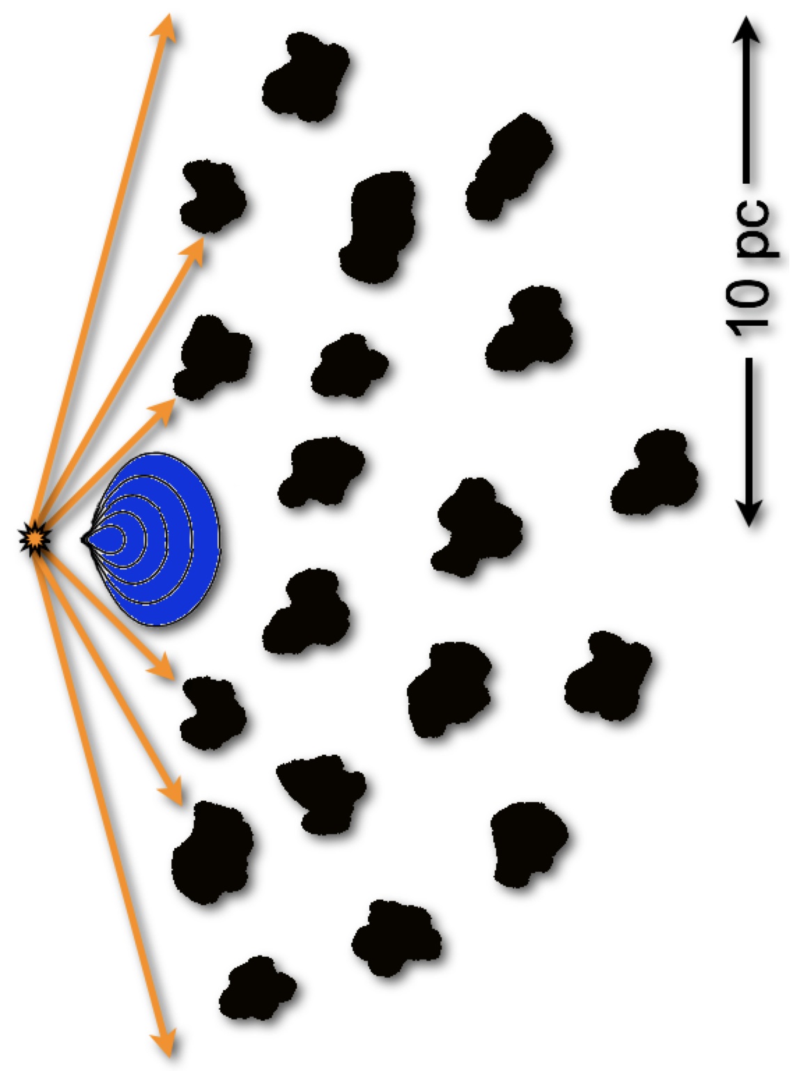
Figure 1: Sketch of the central region of a Seyfert nucleus as found in the 3D simulations done in Schartmann et al. (2010).

In Sect. 2, we describe the numerical model and physical setup of our simulations and explain the test problems we used to assess their accuracy. Sect. 3 describes our simulations and the main results of our parameter studies. It is followed by a critical discussion in Sect. 4, before we conclude in Sect. 5.

2 Model and test calculations

2.1 The approximative radiative transfer approach

Even with today’s computational power the simultaneous solution of the hydrodynamical evolution and the time-dependent radiative transfer equation is impractical for high-resolution multi-dimensional simulations. Severe simplifications have to be applied, depending on the problem under investigation.

In the simulations shown here, we explore the situation of a strong point source, illuminating a spatially confined cloud, immerged at a distance of several tens of dust sublimation radii in initially dust-free, low density gas. The spectral energy distribution of the central source peaks in the ultra-violet wavelength regime, where also the mass absorption coefficient of the adopted dust model shows a prominent maximum. Therefore, radiation can only penetrate a relatively short distance into the cloud, before the high energy UV-photons get absorbed and re-emitted in the infrared wavelength regime. By consequence, the surface of the cloud in the direction of the central source will receive almost all of the radiative acceleration. Given the steep drop of the dust temperature distribution at this rim and the fact that the clouds are far away from the sublimation radius, secondary infrared radiation pressure effects are of minor importance for the dynamical evolution in our infalling clump scenario. A second consequence is that radiation pressure effects predominantly act in radial direction and are dynamically unimportant in vertical direction, as long as the dust temperatures are low and the optical depth is not too high. Hence, a one-dimensional treatment of the radiative transfer problem is reasonable here. Furthermore, we are mainly interested in the dynamical evolution and not in the detailed thermodynamics of the dust distribution.

The issues raised above justify the following simplified approach: We treat the central accretion disc as an isotropically radiating point-source with a spectral energy distribution as shown in Fig. 3b of Schartmann et al. (2005), but normalised to correspond to 10% of the Eddington luminosity for the case of the nearby Seyfert 2 galaxy NGC 1068. The radiation is divided into 54 wavelength bins and propagated along radial rays outwards, where we take geometrical dilution and absorption and reemission by the dust grains in each cell into account. Scattering is neglected. A full radiative transfer calculation within each time step is done. We further make a one fluid assumption and fully couple gas and dust dynamically. The reason for this coupling is that dust grains are charged due to the UV and X-ray radiation and couple to the gas with the help of magnetic fields. The effects of grain charging and gas-dust-coupling have been investigated e. g. by Scoville & Norman (1995). We calculate the gas and dust temperatures separately by assuming that no heat is transferred between the gas and the dust phase. Only those cells receive accelerating forces, which possess gas temperatures below a threshold temperature $T_{\mathrm{sputt}}=10^{5}$K. At this temperature, the rates of change of the grain radii of silicate and graphite grains show a steep rise (Dwek et al., 1996), caused by sputtering processes transmitted by the hot gas, they are embedded in. From $T_{\mathrm{sputt}}$ onwards, we assume that the hot gas will destroy the dust content of the given cell instantaneously. Those cells with a density below a gas density threshold $\rho_{\mathrm{gas}}^{\mathrm{thresh}}$ will not be accelerated either (typically chosen to be twice the minimum density threshold of the simulation, see Table 2). Otherwise, this would lead to artificial generation of matter at the inner boundary of the domain due to the lower limit of the gas density in the simulations. These criteria enable us to distinguish between the gas and the dust phase.

2.2 Opacity model

We use a standard galactic dust model, which is split into 54 frequency bins and has averaged dust grain properties. Grain radii vary between 0.005 $\mu$m and 0.25 $\mu$m with a number density distribution proportional to $a^{-3.5}$, where $a$ is the grain radius (Mathis et al., 1977). It comprises of 62.5% of silicate and 37.5% of graphite grains, where for the latter, the anisotropic behaviour is taken into account. Optical constants are adopted from Draine & Lee (1984), Laor & Draine (1993) and Weingartner & Draine (2001). The resulting opacity curve is shown as the dashed line in Fig. 3a of Schartmann et al. (2005). A gas-to-dust mass ratio of 150 is used in the simulations shown in this paper.

2.3 Test simulations

In order to demonstrate the suitability of our numerical approach of simulating radiative effects, we performed a number of test simulations. The most relevant will be discussed in this section.

2.3.1 Radiative transfer

To test the accuracy and validity of our simplified radiative transfer treatment, we compare the resulting temperature distributions with the three-dimensional Monte-Carlo radiative transfer code RADMC-3D (Dullemond, 2010). The computational domain is chosen to have the same physical size and resolution as the cloud simulations described in this paper, but we fill it homogeneously with dust with densities of $\rho_{\mathrm{d}}=10^{-25}\,\mathrm{g}\,\mathrm{cm}^{-3}$, $\rho_{\mathrm{d}}=10^{-24}\,\mathrm{g}\,\mathrm{cm}^{-3}$, $\rho_{\mathrm{d}}=10^{-23}\,\mathrm{g}\,\mathrm{cm}^{-3}$ and $\rho_{\mathrm{d}}=10^{-22}\,\mathrm{g}\,\mathrm{cm}^{-3}$. These correspond to optical depths at a wavelength of $\lambda=9.8\,\mu$m of $\tau_{9.8\mu\mathrm{m}}=0.05$, $0.50$, 4.97 and 49.73, where a dust absorption coefficient of $\kappa_{\mathrm{abs}}^{9.8\mu\mathrm{m}}=16,446.66\,\mathrm{cm}^{2}\mathrm{g}^{-1}$ was used, taken from our frequency dependent dust model, as described in Sect. 2.2.

The resulting radial temperature profiles are plotted in Fig. 2. As expected, our approximate treatment results in lower temperatures compared to the Monte Carlo approach, as we only take forward reemission into account. This effect is stronger for larger optical depths, because reemission becomes increasingly important. The deviations between the two codes are shown graphically in Fig. 3. While the optically thin cases mainly display numerical noise, the deviations reach the ten percent level in-between the $\tau_{9.8\mu\mathrm{m}}=4.97$ and $49.73$ case. The maxima of the deviations of the radial temperature profiles of the test simulations are summarised in Table 1.

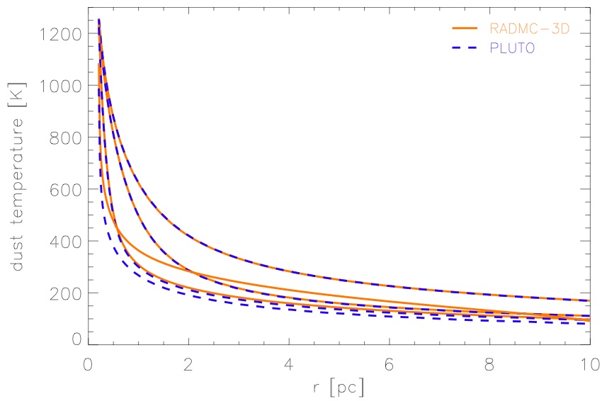
Figure 2: Comparison of the radial dust temperature distribution for an optical depth varying between $\tau_{9.8\mu\mathrm{m}}=0.05$ (uppermost blue dashed curve) to $\tau_{9.8\mu\mathrm{m}}=49.73$ (lowermost blue dashed curve) in steps of a factor of 10 within a homogeneous, spherical distribution of dust. The blue dashed lines show the result of our approximate radiative transfer solver, whereas the orange solid lines represent the reference solution calculated with RADMC-3D (Dullemond, 2010).

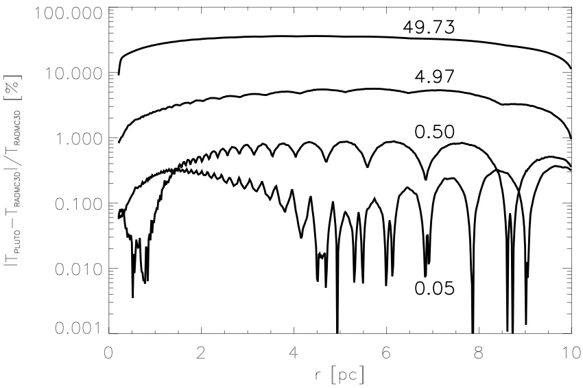
Figure 3: Deviation of the solution of our approximate 1D radiative transfer treatment within the PLUTO code (Mignone et al., 2007) with the resulting temperature distribution derived with RADMC-3D (Dullemond, 2010), given in % for the four optical depths $\tau_{9.8\mu\mathrm{m}}$, as indicated in the plot (compare to Fig. 2).

Table 1: Accuracy of the radial temperature distribution.

$\tau_{9.8\mu\mathrm{m}}$	$\frac{T-T_{\mathrm{ref}}}{T_{\mathrm{ref}}}$ [%]
0.05	0.37
0.50	0.88
4.97	5.63
49.73	36.06

Maximum deviations of the radial temperature distribution calculated with the one-dimensional approximative radiative transfer routine implemented in PLUTO (Mignone et al., 2007) and the reference calculation, done with RADMC-3D (Dullemond, 2010) for the four different optical depths tested.

2.3.2 Radiation pressure acceleration

To test the radiation pressure acceleration, we set up a one dimensional dusty shell and illuminate it from the centre, without taking gravitational forces into account. The domain is set up as in our standard model (see Sect. 2.4). The shell is initially located at a radial distance between 4.5 pc and 5.5 pc. We fill the shell homogeneously with our standard gas and dust mixture with a density, such that the dust optical depths in radial direction (through the whole model space) lie between 0.1 and 10,000 at a wavelength of $9.8\,\mu$m.

Assuming an optically thick shell of gas and dust and no acceleration mechanism other than radiation, we analytically expect an acceleration of the shell of the following form:

$$a_{\mathrm{rad}}=\frac{L_{\mathrm{AGN}}}{4\,\pi\,r^{2}\,c}\,\frac{1}{N\,\mu}$$ (1)

where $L_{\mathrm{AGN}}$ is the bolometric luminosity of the central accretion disc, $r$ is the distance to the centre, $c$ is the speed of light, $N$ the gas column density and $\mu$ the mean particle mass of the gas. With the assumptions made in this article, the gas column density is directly related to the optical depth by

$$N=9.15\cdot 10^{21}\,\mathrm{cm}^{-2}\,\frac{0.60\,m_{\mathrm{a}}}{\mu}\,\frac{16,446.66\,\mathrm{cm}^{2}\mathrm{g}^{-1}}{\kappa}\,\frac{f_{\mathrm{gtd}}}{150.}\,\tau,$$ (2)

where $m_{\mathrm{a}}$ is the atomic mass unit and $f_{\mathrm{gtd}}$ is the gas-to-dust mass ratio. Given the spherical expansion of the shell, the column density will scale with $r^{-2}$ and a constant acceleration with time is expected.

We compare this analytical estimate (thick red lines) with the result of our approximative radiation pressure treatment (black symbols) in Fig. 4 in terms of the time evolution of the density weighted velocity of the shell. For this study, the initial dust optical depth is varied between $\tau_{9.8\mu\mathrm{m}}=$ 0.1 and 10,000, as annotated in the figure. For the analytical estimate, the column density is determined from the simulations for each individual time step.

Very good agreement is found for the highest optical depth case. Towards lower optical depths, we find two competing effects: (i) in these adiabatic test calculations, pressure effects due to the compression of the inner boundary layer of the shell increase with decreasing optical depth and get dynamically significant, leading to an additional acceleration and (ii) at some point, the shell gets optically thin and less and less radiation flux is absorbed and can contribute to acceleration of the shell. At this point, our analytical estimate is invalid and the goodness of the dynamical evolution of our approach can be judged by the correctness of the radial temperature distribution (see Fig. 2 and 3). As both of these effects are not present for the case of the highest optical depth, the best agreement is found for these cases. Thus, we have demonstrated that our approach produces reasonable radial radiative accelerations for the simulations presented in this paper.

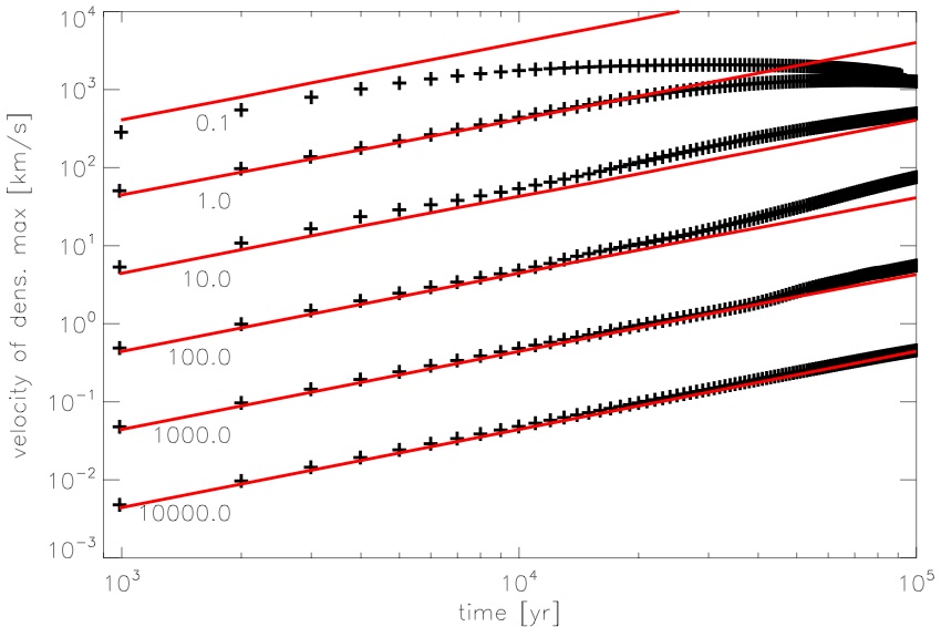
Figure 4: Time evolution of the density weighted velocity around the density maximum ($\rho>0.01\,\rho_{\mathrm{max}}$) of an initially homogeneous shell (black symbols), compared to the analytically expected behaviour (velocity $\propto$ time, thick red lines) for different initial total optical depths (at $\lambda=9.8\,\mu$m), as annotated.

2.4 Numerical Setup

The initial cloud configuration is chosen to represent a typical clump as seen in the three-dimensional torus simulations by Schartmann et al. (2010), as mentioned in Sect. 1, but with the density adjusted to be close to the transition between in- and outflow. Those simulations had been prepared to represent the core region of the nearby Seyfert 2 galaxy NGC 1068. For the sake of simplicity and to derive the basic behaviour, spherically symmetric clouds are assumed, with a homogeneous or initially Gaussian density distribution. They are located at a few parsec distance from the central source and have typically radii of the order of one parsec. Their kinematics is dominated by radial infall motion and we neglect any overlayed orbital motion around the centre. The gravitational potential is the same as in Schartmann et al. (2010) and comprises of a supermassive black hole at the centre with $8\cdot 10^{6}\,\mathrm{M}_{\odot}$ and a nuclear star cluster with a Plummer potential with a core radius of $25\,$pc and a total mass normalisation constant of $2.2\cdot 10^{8}\,\mathrm{M}_{\odot}$. The basic parameters of the studies shown in this article are listed and described in Table 2.

Table 2: Basic parameters of our simulations.

name	$r_{\mathrm{initial}}$ [pc]	$R_{\mathrm{cloud}}$ [pc]	$r_{\mathrm{in}}$ [pc]	$r_{\mathrm{out}}$ [pc]	$\sigma_{\mathrm{c}}$ [pc]	$n_{\mathrm{res}}$	$\rho_{\mathrm{cloud}}[\frac{\mathrm{g}}{\mathrm{cm}^{3}}]$	$\rho_{\mathrm{min}}[\frac{\mathrm{g}}{\mathrm{cm}^{3}}]$	EOS	$\epsilon_{\mathrm{edd}}$	$\tau_{9.8\mu\mathrm{m}}$
SC00	5	1	0.2	10	0	512	1.0e-19	1.0e-23	cool.	0.1	67.4
SC01	5	1	0.2	10	0	512	5.0e-20	5.0e-24	cool.	0.1	33.7
SC02	5	1	0.2	10	0	512	2.5e-20	2.5e-24	cool.	0.1	16.8
SC03	5	1	0.2	10	0	512	1.0e-19	1.0e-23	isoth.	0.1	67.4
SC04	5	1	0.2	10	0	512	1.0e-19	1.0e-23	adiab.	0.1	67.4
SC05	5	1	0.2	10	0.25	512	1.0e-19	1.0e-23	cool.	0.1	21.2
SC06	5	1	0.2	10	0.50	512	1.0e-19	1.0e-23	cool.	0.1	40.5
SC07	5	1	0.2	10	1.00	512	1.0e-19	1.0e-23	cool.	0.1	57.7
SC08	5	1	0.2	10	0	512	1.0e-19	1.0e-23	cool.	0.2	67.4
SC09	5	1	0.2	10	0	256	1.0e-19	1.0e-23	cool.	0.1	68.7
SC10	5	1	0.2	10	0	1024	1.0e-19	1.0e-23	cool.	0.1	67.7
SC11	5	1	0.2	20	0	512	2.5e-20	2.5e-24	cool.	0.1	16.9
TC00	5 & 8	1	0.2	10	0	512	5.0e-20	5.0e-24	cool.	0.1	33.7 & 34.0

$r_{\mathrm{initial}}$ is the initial distance of the cloud centre from the black hole, $R_{\mathrm{cloud}}$ is the cloud radius, $r_{\mathrm{in}}$ and $r_{\mathrm{out}}$ are the inner and outer radius of the computational domain, $\sigma_{\mathrm{c}}$ is the cloud density concentration parameter in case of a Gaussian distribution (zero for a constant density cloud), $n_{\mathrm{res}}$ is the number of resolution elements in radial and theta direction, $\rho_{\mathrm{cloud}}$ is the gas density of the cloud, $\rho_{\mathrm{min}}$ is the lower gas density threshold in the simulation, EOS is the equation of state and $\epsilon_{\mathrm{edd}}$ is the Eddington ratio of the central radiation source, $\tau_{9.8\mu\mathrm{m}}$ is the optical depth through the centre of the initial cloud at $9.8\,\mu$m. Bold face indicates parameter changes with respect to our standard model.

To evolve the hydrodynamical equations, we use the fully parallel high-resolution shock-capturing scheme PLUTO (Mignone et al., 2007). For the calculations shown in this paper, the two-shock Riemann solver was chosen together with a linear reconstruction method and directional splitting. Optically thin cooling is included with the help of an effective cooling curve for solar metallicity (see Fig. 1 in Schartmann et al. (2009) and text therein). All boundary conditions are set to outflow, not allowing for inflow. We do not take magnetic fields into account in these calculations. In these two-dimensional simulations, we cannot investigate the dependence of the radiation pressure effects on cloud rotation (see discussion in Sect. 4).

3 Results

3.1 Cloud evolution

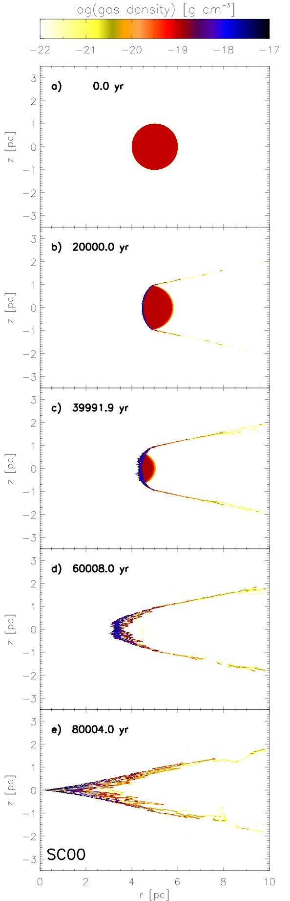
Figure 5: Time evolution of the gas density distribution for our standard model (simulation SC00). Labels are given in parsec, the time is given in years. The cloud gets initially compressed and moves inwards.

Fig. 5 and the upper row of Fig. 8 show the time evolution of the density distribution for our standard model (SC00) in Cartesian as well as spherical coordinates. After having switched on the central radiation source, the initially spherical cloud (Fig. 5a) contracts in radial direction (Fig. 5b). The inner boundary of the cloud experiences direct radiation pressure interaction, which produces a nearly isothermal shock wave with a compression factor of about a hundred. The outer part of the cloud, which is well shielded from the central radiation source still experiences the gravitational forces and is accelerated inwards. These two effects together result in a converging flow, which causes the formation of density fluctuations by a number of fluid instabilities (Fig. 5c). Most important in this case is the non-linear thin shell instability (NLTSI), the Kelvin-Helmholtz-instability (KHI) and the thermal instability. For a detailed description we refer to Heitsch et al. (2006). As the pressure in the cloud rises above the ambient pressure, the cloud expands in the direction perpendicular to the radial direction. This gas, together with other low density gas at the upper and lower cloud edge is stripped and forms long, radial tails which are subject to Kelvin-Helmholtz-instabilities (Fig. 5d,e). These, together with shielding effects lead to the formation of a turbulent wake and some mixing of higher density clumps into the shadow region of the cloud. The onset of turbulence is suppressed in regions with direct lines-of-sight towards the radiation source, as this relatively low density material suffers from strong outward acclerations. With the given parameters, the centre of mass (COM) of the cloud starts moving inwards. As radial rays with lower column densities suffer from a higher radiation pressure acceleration (Equ. 1), they lag behind. This leads to the formation of a narrow, sickle shaped structure (Fig. 5c,d). An additional structuring effect results from the gas cooling. Dense regions cool on shorter timescale ($t_{\mathrm{cool}}\propto\frac{1}{\rho}$), leading to further contraction. As a result of this cooling instability, density inhomogeneities within the converging flow are able to contract further, finally forming small cloudlets of high density material. As the acceleration critically depends on the column density of the material (see equation 1), the shell is now able to spread out again (Fig. 5d,e), forming radially extended filaments and high density knots, which show a strong dependence on the balance between gravitational and radiation pressure acceleration forces. In principle, each cloudlet now goes through an evolution similar to our initial cloud.

In summary, three different phases of cloud evolution are observed: (i) radiation pressure and gravitational forces lead to a compression of the cloud in radial direction, leading to a lenticular shape (the lense phase, Fig. 5b,c), (ii) the converging flows at the inner edge together with cooling of the gas lead to a clumpy, sickle-shaped distribution (the clumpy sickle phase, Fig. 5c,d) and (iii) the clumps induce a column density instability, which stretches the cloudlets into long radial filaments (the filamentary phase, Fig. 5d,e).

Fig. 6 shows the evolution of the distribution of mass onto spherical shells (given as a fraction of the initial total mass in the computational domain) in this model. The initial distribution is given in black, whereas the other colors are used for later snapshots, as indicated in the legend of the plot. It quantifies the behaviour as already described above: first of all, radiation pressure leads to a density maximum at the inner boundary, whereas the unaffected cloud still gets accelerated towards the centre, leading to a converging flow. Altogether, the mass distribution gets narrower in radial direction (concerning the bulk of the gas). As soon as the clumpy structure has evolved, the various column densities in radial direction lead to slightly varying radial velocities for different theta angles. This can be seen as an increase of the width of the profile, as visible for the case of the red curve. By that time (80,000 yr after the start of the simulation), parts of the filaments have already reached the sublimation radius, which approximately coincides with the inner boundary in our simulations.

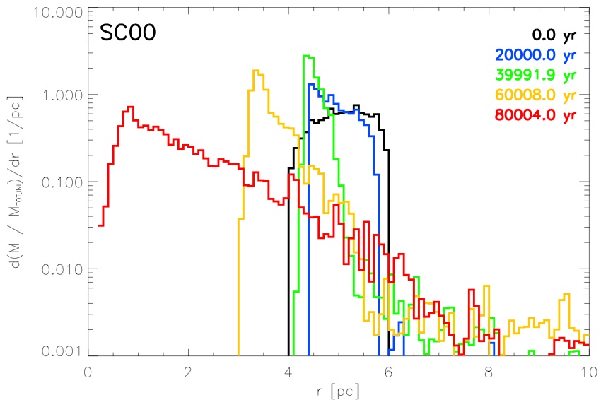
Figure 6: The evolution of the distribution of mass onto spherical shells is shown for model SC00 for five different time snapshots, as indicated in the legend.

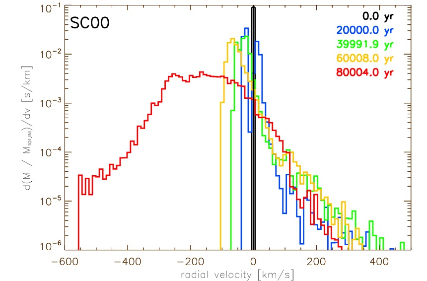
Figure 7: Mass histogram of the radial velocity distribution of our standard model (SC00).

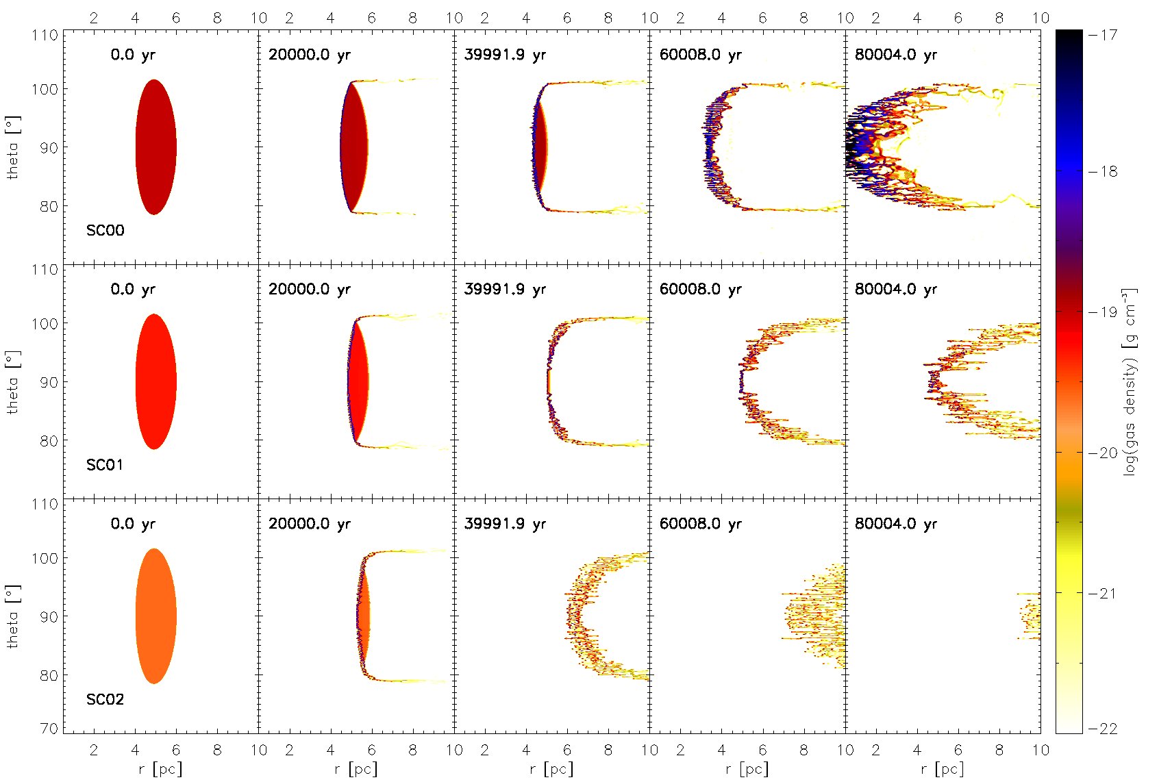
Figure 8: Density evolution for clouds with various masses. Shown are the three simulations SC00 ($\rho_{\mathrm{cloud}}=1\cdot 10^{-19}$g $\mathrm{cm}^{-3}$, upper row), SC01 ($\rho_{\mathrm{cloud}}=5\cdot 10^{-20}$g $\mathrm{cm}^{-3}$, middle row) and SC02 ($\rho_{\mathrm{cloud}}=2.5\cdot 10^{-20}$g $\mathrm{cm}^{-3}$, lower row).

The differential gas mass distribution as a function of the radial velocity is shown in Fig. 7. Initially, the cloud is at rest (black line). The various colours show different timesteps as indicated in the legend. With time, the distribution broadens. The bulk of the mass is accelerated inwards, whereas a small fraction (at the low column density edges of the cloud) gets accelerated outwards. This is again caused by the vertical small scale variations of the column density. Most of the mass is contained in the inward accelerated dense cloudlets, whereas the low density tails contribute only little to the total mass budget.The cutoff at large infall velocities is caused by the fact, that part of the material has already left the model space.

3.2 Cloud density study

Fig. 8 shows the time evolution of the density distribution of a cloud density study, displayed in spherical coordinates. The cloud’s column density was chosen such that the clouds are close to force equilibrium between the gravitational and radiation pressure force. The first row corresponds to the standard model (SC00) discussed in Sect. 3.1. For the second and third row, we halved (SC01) and quartered (SC02) the density of the cloud respectively. Within the density range shown, all three basic evolutionary phases discussed above can be recognized, but several distinct differences exist: As expected, the motion of the centre of mass changes and the inward motion is slower for lower density values and reaches a transition to outflow after a column density threshold is reached (see Sect. 3.3). For the case of the outflowing cloud (SC02), we also see a larger spread of the sickle-shaped cloud in radial direction. For the case of even higher column densities than displayed, the amount of compression decreases, as gravitational acceleration dominates over radiation pressure effects. Radiation pressure effects are only effective at the cloud edges, where cometary-shaped tails build up, which develop Kelvin-Helmholtz-instabilities and form a turbulent wake behind the cloud. Only the inner boundary of the cloud forms small cloudlets and filaments, whereas the outer part keeps a continuous density distribution. On its way towards the centre, the cloud shrinks due to gravitational forces, gas cooling and the ablation of gas at the outer edges.

In summary, clouds can encounter two fates, depending on their radial column density: (i) Low column density clouds will be pushed outwards, whereas (ii) high column density clouds always show both, in- and outflow motion, due to the formation of tails at the low column density edges of the clouds.

Fig. 9 shows the radial distribution of mass for clouds with different densities for an early snapshot (upper panel, after 20,000 yr) and a late snapshot (lower panel, after 60,000 yr). It clearly shows the dependence of the density distribution on the initial condition: whereas the high density case remains peaked, it spreads out more and more for the lower column density clouds.

The shearing of the cloud is quantified in Fig. 10. First of all, we determine the centre of mass of the cloud. Then we add up the mass in the spherical shell defined by the radial cell, which contains the COM. We extend the spherical shell (symmetrically with respect to the centre of mass) until it includes 50% of the mass of the initial condition within the spherical shell embracing the initial cloud. This is done for the standard model (SC00, black line), the model with half the mass of the standard model (SC01, blue line) and a model with a quarter of the mass of the standard model with an outer radius extended to 20 pc (SC11, red line). In the beginning of the simulation, the contraction of the cloud is visible, before the differential forces lead to a shearing. Two types of shearing occur: (i) due to the column density differences between the cloud centre and the cloud’s outer edge, as visible in the extended tails and (ii) due to the small scale column density differences which emerge in a later stage of the evolution. After the compression phase, the half mass shell size increases almost linearly for the case where the COM moves outward (see Fig. 11). The evolution is fastest for the low density case, where radiation pressure dominates the radial forces. The infalling high density case behaves differently, as the dense inner shell which forms due to the initial contraction seems to prevent efficient shearing.

Fig. 12 quantifies the different velocities reached. Whereas the highest density cores reach the smallest outflow and the highest inflow velocities, respectively, the highest outflow velocities are reached by the material within the tails expelled from the cloud edges. This material shows up as the extended tails of the distributions in Fig. 12.

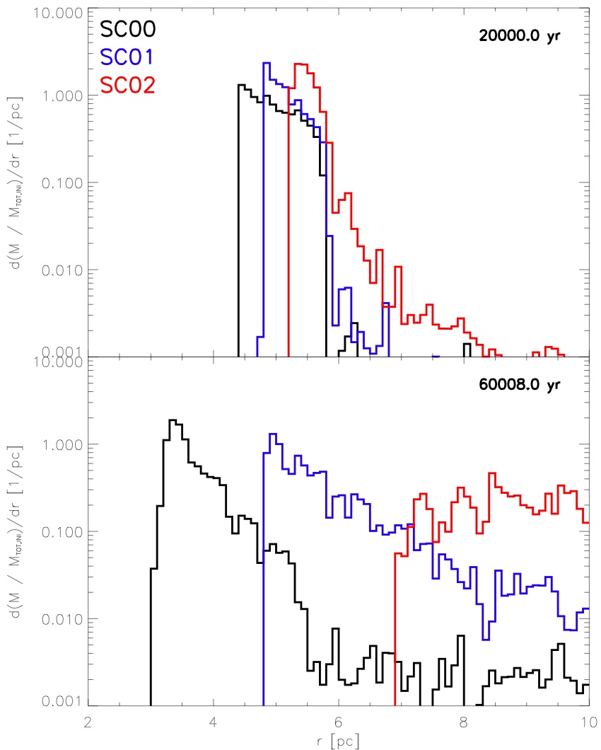
Figure 9: Distribution of mass on spherical shells for a density study. Our standard model (SC00) is given in black, whereas the blue line corresponds to an initial cloud mass of half the standard model’s value (SC01) and the red line to a quarter of it (SC02). It is shown for two time snapshots in the upper and lower panel as indicated in the upper right corner.

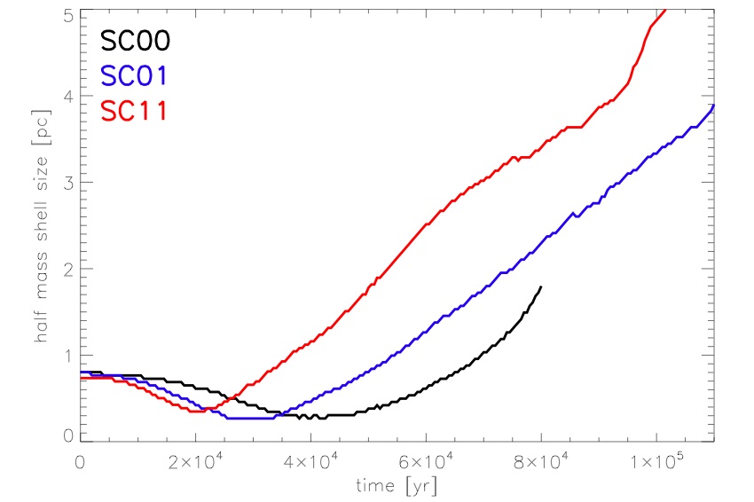
Figure 10: Time evolution of the thickness of the concentrical shell around the origin at the location of the centre of mass, which encloses 50% of the initial mass. SC00 is our standard model, SC01 has half the mass of the standard model and SC11 a quarter of the mass. SC11 is identical to SC02, but we increased the outer radius of the computational domain to 20 pc.

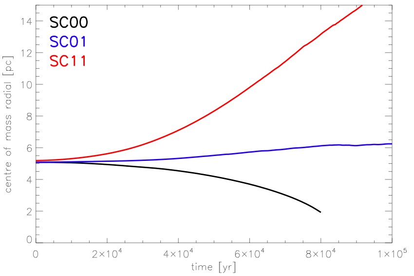
Figure 11: Time evolution of the radial location of the centre of mass for the cloud density study. SC00 is our standard model, SC01 has half the mass of the standard model and SC11 a quarter of the mass. SC11 is identical to SC02, but we increased the outer radius of the computational domain to 20 pc.

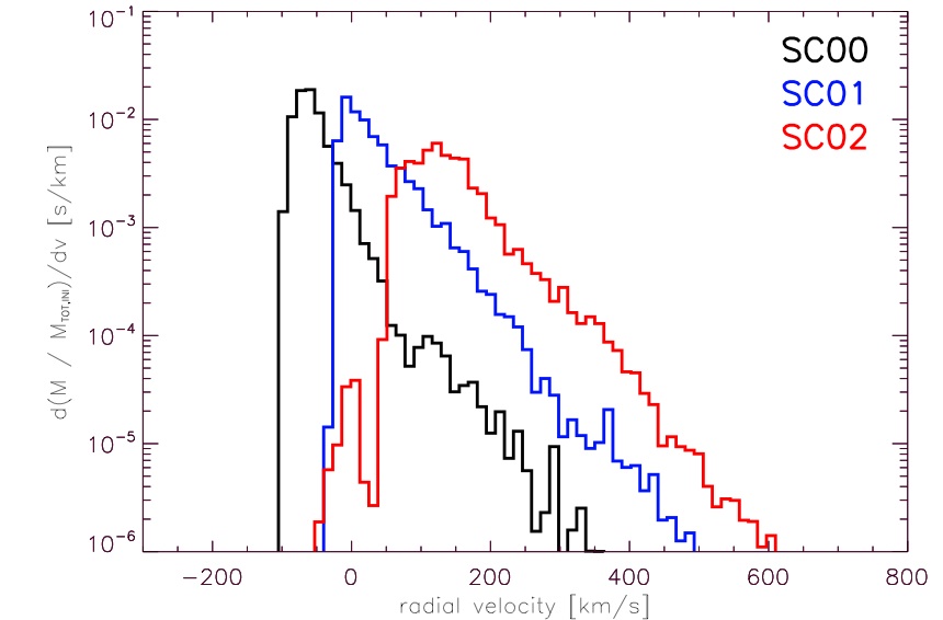
Figure 12: Histograms of the distribution of mass into bins of radial velocity for the cloud density study, after an evolution time of 60,000 yr (SC00 – standard model, SC01 – half the mass, SC02 – a quarter of the mass).

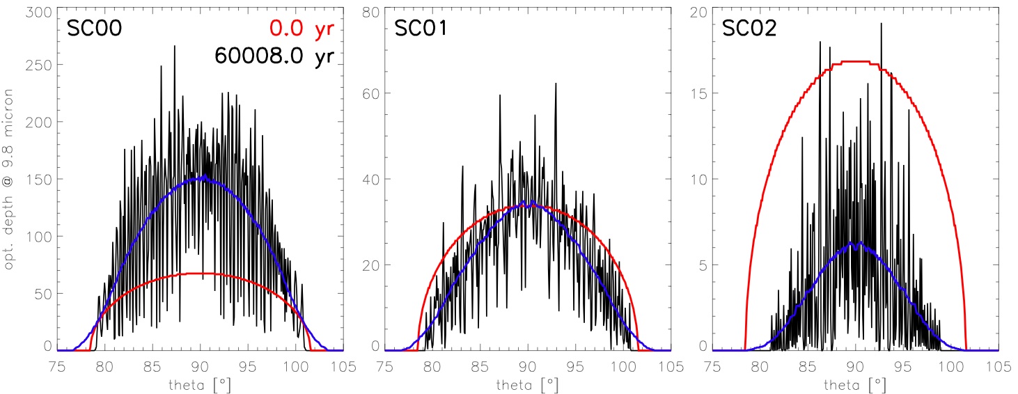
Figure 13: Distribution of the optical depth in radial direction. Shown are the initial distribution (red lines) and the distribution after roughly 60,000 yr (black lines) for the density study (SC00 – standard model, SC01 – half the mass, SC02 – a quarter of the mass). The blue line represents the distribution after 60,000 yr, but smoothed with a boxcar function of 5 degrees width in theta direction.

Fig. 13 shows the evolution of the optical depth (or the column density distribution, compare to Equ. 2) in radial direction for the three simulations of the gas density study. Each panel displays the initial distribution in red and the state after roughly 60,000 yr in black. The overlayed blue line corresponds to the black line, but is smoothed with a boxcar function of 5 degrees width in theta direction. In all three cases, the distribution gets more peaked with respect to the initial distribution. The high density case shows a global increase of the optical depth, while it stays almost constant in simulation SC01 and overall decreases for the case of simulation SC02. Both of these effects are mostly caused by the inward or outward motion of the cloud. Being accelerated inward leads to a contraction of the cloud by gravitational forces, whereas the outward moving cloud expands due to the radially acting radiation pressure forces. As already discussed, the cloud evolves into a sickle shape. Being stretched radially, the edges rather expand, whereas the central parts rather contract, leading to a more peaked distribution of the optical depth. The standard deviation of the distribution of the later snapshot with respect to the smoothed curve drops from 24% of the peak value of the smoothed curve for the high density case to 19% for the intermediate density case and amounts to 44% for the low density case. The intermediate density case is closest to the equilibrium between gravitational and radiation pressure forces leading to only minor inward and outward motion in the early phase. In the other cases, contraction or expansion of the whole cloud leads to enhancement of the column density fluctuations.

3.3 Comparison to analytical expectations

In this section, we compare the general dynamics of the cloud remnant to a simple analytical acceleration model. For the latter, we assume that the clouds retain their initial cross section throughout the whole acceleration process. The cloud absorbs all incident radiation onto its geometrical cross section of $\sigma=\pi\,R_{\mathrm{cloud}}^{2}$. Including the gravitational attraction of the central black hole and the stellar cluster, this results in an accelerating force of

$$F_{\mathrm{acc}}=\frac{L_{\mathrm{AGN}}}{4\,\pi\,r^{2}\,c}\,\sigma-\frac{G\,m_{\mathrm{cloud}}\,M(r)}{r^{2}},$$ (3)

where $L_{\mathrm{AGN}}$ is the luminosity of the central accretion disc, $M(r)=M_{\mathrm{BH}}+\hat{M}_{*}\,\frac{\left(\frac{r}{r_{\mathrm{c}}}\right)^{3}}{\left(1+\left(\frac{r}{r_{\mathrm{c}}}\right)^{2}\right)^{3/2}}$ is the mass of the central supermassive black hole and the nuclear star cluster. The latter is modelled as a Plummer profile with core radius $r_{\mathrm{c}}$. $G$ is the gravitational constant and $c$ the vacuum speed of light. A second order accurate leapfrog algorithm is used to integrate the dynamics of the cloud.

In Fig. 14 we compare the result of this experiment with our simulations. The velocity of the cloud or cloud remnant is shown after an evolution time of roughly 60,000 years for various values of the optical depth through the midplane of the cloud. For the case of the numerical radiation hydrodynamics (RHD) simulations, both values are determined by averaging over 10 grid cells in vertical direction, centered on the midplane. In radial direction, all grid cells, which are filled with dust are taken into account when summing up the optical depth and calculating the median velocity, respectively. Plotted in yellow is the result of the analytical estimate. The black triangles and blue stars refer to our RHD simulations listed in Table 2.

In general, the simulations are in reasonable agreement with the simple analytical estimate. As expected, the agreement is better for the high optical depth case. For decreasing optical depth values, smaller and smaller areas of the clouds fulfill the assumption that all lines of sight through the clouds are optically thick. The deviations arise from the fact that in the real hydrodynamical simulations, the clouds get disrupted by the action of the radiation pressure and gravitational forces together with the onset of instabilities, leading to overall larger sizes and, therefore, smaller column densities and higher outflow velocities.

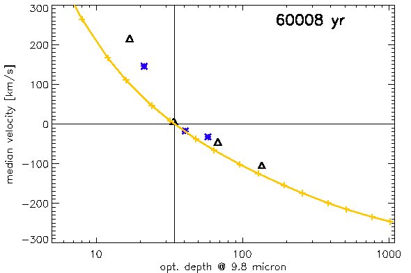
Figure 14: Comparison of our RHD simulations (black triangles for the density study, blue stars for the Gaussian distribution study, see Table 2) and a simple acceleration model of spherical clouds (yellow line and symbols).

3.4 Parameter studies

In the following we summarise the main results from several parameter studies:

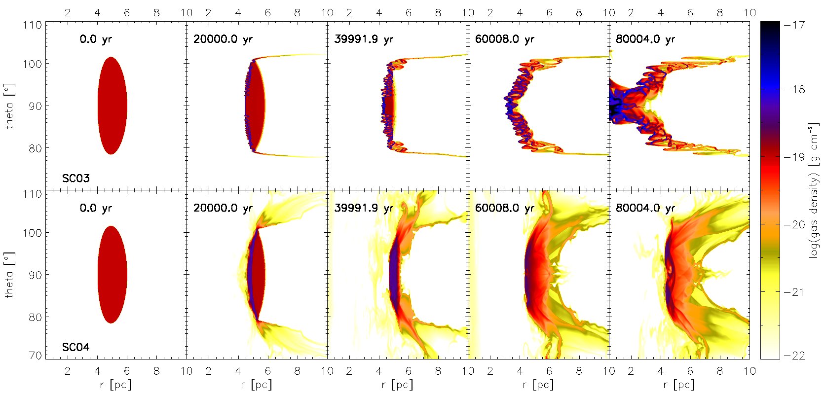
Figure 15: Comparison of the evolution of the density for an isothermal simulation (upper row, SC03) and an adiabatic simulation (lower row, SC04). The parameters are as in our standard simulation (SC00, see Fig. 5 and upper row of Fig. 8).

1. Equation of state:

   For this study, we use the same setup as in our standard model but adopt an isothermal equation of state for each of the two temperature phases of our initial condition or an adiabatic equation of state. The results show substantial differences (see Fig. 15): In the isothermal simulation (upper row, SC03), the converging flow produces a filamentary or clumpy structure as well, but with larger characteristic sizes due to the higher remaining thermal pressure in the cloudlets. This leads to smaller column densities and the cloud reaches smaller infall velocities compared to the case where we take gas cooling into account (Fig. 5). In the adiabatic simulation, which resembles the situation of inefficient gas cooling and efficient gas heating processes, the gas is heated to temperatures above the dust sputtering threshold at the inner edge of the cloud and dust is destroyed. Parts of the cloud are able to evaporate and leave the cloud, as they are not subject to radiation pressure forces anymore in our scheme. Due to the compression in the rim of the cloud, it is now overpressured with respect to the surrounding medium, leading to a slight expansion in vertical direction. As a consequence of the high pressure, the density distribution remains much smoother compared to the cooling case and no strong clumping can occur. Given the lower column density, the cloud’s centre of mass is slightly pushed outwards during the runtime.

2. Gaussian internal structure:

   For this study, we set up a Gaussian internal density distribution ($\rho=\rho_{0}\,\exp{-\frac{(x-r_{\mathrm{initial}})^{2}}{2\,\sigma_{\mathrm{c}}^{2}}}$), where $\rho_{0}$ is the value of the gas density in the centre of the cloud and we vary the concentration parameter $\sigma_{\mathrm{c}}$ from $0.25$ pc to $0.5$ pc and $1$ pc. The stronger the concentration of the mass of the cloud towards the centre, the stronger is the compression of the sickle shape, as the low density outer regions can be pushed outward easily. The cloud centre of mass behaves like expected from the initial midplane column density, which decreases with stronger concentration according to our definition (see Table 2). This can be seen in Fig. 14. The Gaussian internal structure study is shown here as the blue stars.

3. Eddington Ratio:

   

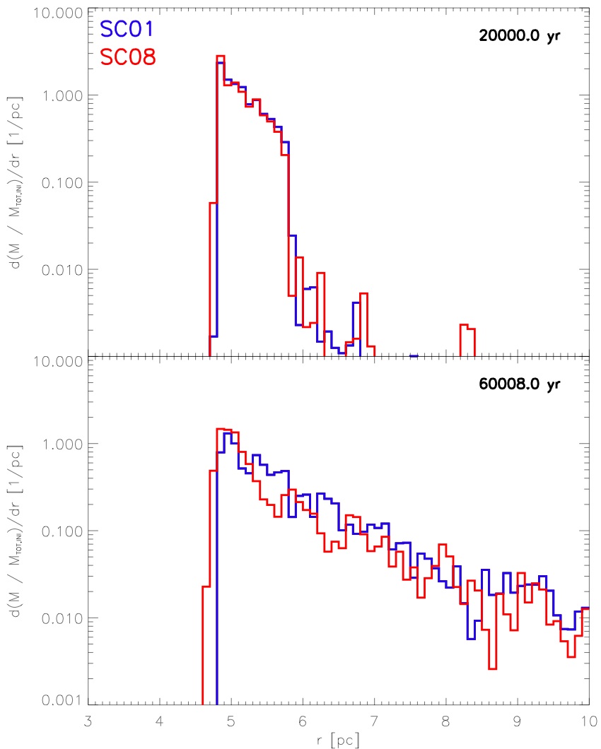
   Figure 16: The distribution of mass onto spherical shells is compared between model SC01 (blue graphs), where the cloud density is half the density of the standard model and SC08 (red graphs), where the luminosity of the central source is twice the luminosity of our standard model. The two panels correspond to two different timesteps.

   As can be seen from equation 1, the radiation pressure acceleration in the optically thick limit scales proportional to the source luminosity $L_{\mathrm{AGN}}$ and to the inverse of the gas column density. Therefore, for the case of the Eddington ratio study, we expect a similar behaviour as for the density study. This is indeed the case, as can be seen from Fig. 16, where the simulation with half of the mass of the standard model (SC01, blue line) is compared to the standard model illuminated with twice the source luminosity (SC08, red line).

3.5 Interacting clouds

In order to study two interacting clouds, we use the same cloud characteristics as in model SC01, but offset the cloud slightly in polar direction. The second cloud (identical to the first one) is placed at a location of 8 pc from the centre and offset by one cloud radius in polar direction. In Fig. 17, the evolution of the density for this setup is shown for a number of snapshots. During the first steps of the evolution, the inner cloud evolves as described in Sect. 3.1. Being optically thick, it casts a shadow on parts of the outer cloud, which – in consequence – reacts only to the gravitational acceleration in this part. In the transition region between shadowed and unshadowed part, the tail of the inner cloud interacts with the outer cloud, punching a hole into it due to the additional ram pressure. For the cloud parameters shown here, the two clumps will collide, leading to the formation of cloudlets with high enough column density to lead to inflow motion.

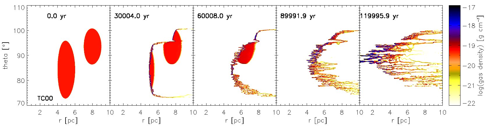
Figure 17: Time evolution of the density distribution for the scenario of two interacting clouds (simulation TC00).

3.6 Resolution study and numeric parameters

A resolution study has been conducted where we decreased the number of grid cells to $256^{2}$ (SC09) and doubled it to $1024^{2}$ (SC10) with respect to our standard model. As expected, the clumpiness of the dense shell depends on the resolution. However, the overall behaviour of the cloud, concerning acceleration, mass distribution and radial velocity is very similar. The higher resolved clouds show a slightly broader distribution of mass along the force direction. There, the column density instability can act on shorter time scales, spreading out the remaining cloud in radial direction. We also find a resolution dependence in the maximum density, as expected.

Several other studies have been undertaken in order to investigate the influence of the numerics on the results of this work. Changing the minimum gas temperature of the simulation changes the minimum size of the cloudlets. The higher we choose this threshold value, the smoother the cloud appears. Clumps continue to form due to the converging flow.

By increasing the density of the surrounding medium, at some point, its cooling time is small enough to form small clumps, which overcome the density threshold for radiation pressure interaction in our simulations. With their ram pressure, they lead to a faster formation of filaments in the cloud.

4 Discussion

In this paper, we investigated the radiation pressure interaction of infalling dusty gas clouds with the active nucleus of a Seyfert galaxy, exemplified for the physical parameters of NGC 1068. Dictated by the gas column density, clouds will be accreted or expelled from the central region. Outward accelerated clouds will interact and merge with clouds and filaments further out, until the critical column density is reached. Fig. 18 shows the column density distribution in radial direction for the 3D model of the Seyfert 2 galaxy NGC 1068 as discussed in Schartmann et al. (2010). It is shown for all polar angles, each of them averaged over the azimuthal angle. Clearly visible is the two-component structure – the geometrically thin, but high-column density disc and the extended low-column density torus on tens of parsec scale. The dark blue dotted line denotes the transition between in- and outflow motion as derived in this article. The latter is only a rough estimate, as it neglects the radius dependence given by the extended potential of the nuclear star cluster. The light blue dashed line shows the same column density threshold, but assuming a radiation characteristic of the source proportional to $|cos(\vartheta)|$. According to this column density distribution, most of the large scale filamentary torus component would be expelled from the central region, as it is unshielded by the central parsec scale disc component. The red line refers to a model, where we distributed the material in the disc (up to a distance from the black hole of 2 pc and an angle of $\pm 45\degr$ with respect to the disc midplane) in a wedge-shaped structure with a 45 degree half opening angle. This should resemble the geometrically thick dusty torus, which would result from our inner disc component, if the scaleheight would have been increased by a thus far unknown turbulent process. As can be seen from Fig. 18, a large fraction of the model space is then sufficiently shielded to allow for further feeding of the central galactic region, whereas gas far away from the midplane will still be pushed outward.

For all of the simulations shown in this paper, we assume that gas and dust are thermally decoupled. This is strictly true only up to a threshold density of $10^{-18}\,\mathrm{g}\,\mathrm{cm}^{-3}$ (Larson, 2005). At high densities, the gas temperature is given by the heating and cooling processes of the dust. This limit is taken into account only very roughly in our simulations by setting up a minimum gas temperature, which affects the minimal extension of the cloudlets.

In this first set of models, we neglect magnetic fields mainly for the sake of simplicity. Despite this, magnetic fields are supposed to be important in these galactic nuclear regions, but their strengths and morphologies are basically unknown. In the context of such simulations of dusty clouds, two main effects are expected: (i) magnetic fields provide an additional pressure component and (ii) the interaction of magnetic fields with charged ions and dust grains leads to a strong coupling of the gas and dust phase (e. g. Scoville & Norman, 1995). The latter enables us to treat the two phases in a one-fluid approximation. The clouds we simulate in this paper contain the products of stellar evolutionary processes. Many expelled outer atmospheres of AGB stars have merged to form a larger entity. As these stellar atmospheres were observationally found to be significantly magnetised (e. g. Gómez et al., 2009 and references therein) by stellar dynamos at the interface of the rapidly rotating core and the more slowly rotating envelope (Blackman et al., 2001), the clouds will be magnetised as well. Depending on the (unknown) morphology of the magnetic field lines, their presence may or may not have a stabilising effect on the cloud, which is exposed to radially compressing gravitational and radiative pressure forces. The hot and highly ionised ambient medium is also likely to be magnetised, which might provide an additional confining magnetic pressure, resulting in enhanced stability of the cloud. This scenario was proposed by Rees (1987) to be the dominant confinement mechanism for BLR clouds.

We also neglect the possibility that clouds are rotating. Depending on the rotation frequency compared to the cloud distortion time due to radiation pressure and gravity, this can have a significant effect on the evolution of the cloud and might lead to a different dynamical behaviour of the centre of mass of the cloud. However, to study this, three-dimensional simulations are necessary and we defer this to our future work.

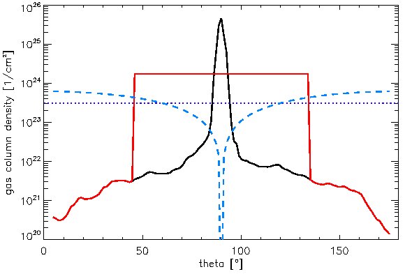
Figure 18: Gas column density distribution of the 3D torus simulations presented in Schartmann et al. (2010) (black line), compared to the approximate column density threshold as derived numerically in this article (dark blue dotted line) and taking the $|\cos(\vartheta)|$-radiation characteristic into account (light blue dashed line). For the case of the red line, we distributed the mass of the central disc within a geometrically thick disc structure, which brings the distribution well above the threshold.

5 Conclusions

With the help of three-dimensional hydrodynamical simulations considering the effects of stellar evolutionary processes of a nuclear star cluster on the surrounding interstellar medium (ISM), Schartmann et al. (2009); Schartmann et al. (2010) typically find a two-component structure: a geometrically thin, but optically thick disc on sub-pc to pc scale, surrounded by a filamentary or clumpy distribution on tens of parsec scale. Building up on these results, we investigate the further evolution of these clumps and filaments after the activation of the central nucleus, employing a simplified treatment: spherical clouds are studied taking gravitational forces, radiative transfer effects and optically thin line cooling into account.

The evolution of the clouds can be separated into three different phases:

1. the lense phase: counteracting forces (radiation pressure and gravity) transform the cloud into a lenticular shape

2. the clumpy sickle phase: due to converging flows and cooling instability, a number of cloudlets form in a sickle-shape, whose general structure is dictated by the initial internal column density distribution of the cloud

3. the filamentary phase: the strung cloudlets introduce a column density instability, leading to the formation of long radial filaments.

The fate of the clouds ultimately depends on the column density of the matter. In summary, two scenarios are possible: (i) low column density clouds will be completely pushed outwards and (ii) high column density clouds loose part of their material at the edges, whereas the bulk of the matter moves inwards. The general dynamical evolution of the cloud can approximately be described with the help of a simple analytical model, where the gas column density determines whether the cloud will move inward or will be pushed outward.

References

- Alig et al. (2011) Alig C., Burkert A., Johansson P. H., Schartmann M., 2011, ArXiv e-prints, accepted by MNRAS
- Blackman et al. (2001) Blackman E. G., Frank A., Markiel J. A., Thomas J. H., Van Horn H. M., 2001, Nature, 409, 485
- Bonnell & Rice (2008) Bonnell I. A., Rice W. K. M., 2008, Science, 321, 1060
- Burtscher et al. (2009) Burtscher L., Jaffe W., Raban D., Meisenheimer K., Tristram K. R. W., Röttgering H., 2009, Astrophys. J., Lett., 705, L53
- Davies et al. (2007) Davies R. I., Mueller Sánchez F., Genzel R., Tacconi L. J., Hicks E. K. S., Friedrich S., Sternberg A., 2007, Astrophys. J., 671, 1388
- Draine & Lee (1984) Draine B. T., Lee H. M., 1984, Astrophys. J., 285, 89
- Dullemond (2010) Dullemond C. P., , 2010, RADMC-3D, http://www.mpia.de/homes/dullemon/radtrans/radmc-3d/
- Dwek et al. (1996) Dwek E., Foster S. M., Vancura O., 1996, Astrophys. J., 457, 244
- Elitzur & Shlosman (2006) Elitzur M., Shlosman I., 2006, Astrophys. J., Lett., 648, L101
- Gómez et al. (2009) Gómez Y., Tafoya D., Anglada G., Miranda L. F., Torrelles J. M., Patel N. A., Hernández R. F., 2009, Astrophys. J., 695, 930
- Heitsch et al. (2006) Heitsch F., Slyz A. D., Devriendt J. E. G., Hartmann L. W., Burkert A., 2006, Astrophys. J., 648, 1052
- Hobbs & Nayakshin (2009) Hobbs A., Nayakshin S., 2009, Mon. Not. R. Astron. Soc., 394, 191
- Hönig et al. (2010) Hönig S. F., Kishimoto M., Gandhi P., Smette A., Asmus D., Duschl W., Polletta M., Weigelt G., 2010, Astron. Astrophys., 515, A23+
- Hopkins & Quataert (2010) Hopkins P. F., Quataert E., 2010, Mon. Not. R. Astron. Soc., 407, 1529
- Laor & Draine (1993) Laor A., Draine B. T., 1993, Astrophys. J., 402, 441
- Larson (2005) Larson R. B., 2005, Mon. Not. R. Astron. Soc., 359, 211
- Mathis et al. (1977) Mathis J. S., Rumpl W., Nordsieck K. H., 1977, Astrophys. J., 217, 425
- Mignone et al. (2007) Mignone A., Bodo G., Massaglia S., Matsakos T., Tesileanu O., Zanni C., Ferrari A., 2007, Astrophys. J., Suppl. Ser., 170, 228
- Norman & Scoville (1988) Norman C., Scoville N., 1988, Astrophys. J., 332, 124
- Prieto et al. (2010) Prieto M. A., Reunanen J., Tristram K. R. W., Neumayer N., Fernandez-Ontiveros J. A., Orienti M., Meisenheimer K., 2010, Mon. Not. R. Astron. Soc., 402, 724
- Rees (1987) Rees M. J., 1987, Mon. Not. R. Astron. Soc., 228, 47P
- Sanders (1981) Sanders R. H., 1981, Nature, 294, 427
- Schartmann et al. (2010) Schartmann M., Burkert A., Krause M., Camenzind M., Meisenheimer K., Davies R. I., 2010, Mon. Not. R. Astron. Soc., 403, 1801
- Schartmann et al. (2005) Schartmann M., Meisenheimer K., Camenzind M., Wolf S., Henning T., 2005, Astron. Astrophys., 437, 861
- Schartmann et al. (2009) Schartmann M., Meisenheimer K., Klahr H., Camenzind M., Wolf S., Henning T., 2009, Mon. Not. R. Astron. Soc., 393, 759
- Scoville & Norman (1988) Scoville N., Norman C., 1988, Astrophys. J., 332, 163
- Scoville & Norman (1995) Scoville N., Norman C., 1995, Astrophys. J., 451, 510
- Seyfert (1943) Seyfert C. K., 1943, Astrophys. J., 97, 28
- Shlosman et al. (1990) Shlosman I., Begelman M. C., Frank J., 1990, Nature, 345, 679
- Tristram et al. (2007) Tristram K. R. W., Meisenheimer K., Jaffe W., Schartmann M., Rix H.-W., Leinert C., Morel S., Wittkowski M., Röttgering H., Perrin G., Lopez B., Raban D., Cotton W. D., Graser U., Paresce F., Henning T., 2007, Astron. Astrophys., 474, 837
- Tristram et al. (2009) Tristram K. R. W., Raban D., Meisenheimer K., Jaffe W., Röttgering H., Burtscher L., Cotton W. D., Graser U., Henning T., Leinert C., Lopez B., Morel S., Perrin G., Wittkowski M., 2009, Astron. Astrophys., 502, 67
- Weedman (1977) Weedman D. W., 1977, Ann. Rev. Astron. Astrophys., 15, 69
- Weingartner & Draine (2001) Weingartner J. C., Draine B. T., 2001, Astrophys. J., 548, 296