Selected Topics in Three- and Four-Nucleon Systems

Abstract

Two different aspects of the description of three- and four-nucleon systems are addressed. The use of bound state like wave functions to describe scattering states in $N-d$ collisions at low energies and the effects of some of the widely used three-nucleon force models in selected polarization observables in the three- and four-nucleon systems are discussed.

1 Introduction

Detailed studies in the three- and four-nucleon systems gives valuable information of the underlying nuclear interaction. These two systems have three bound states, ³H, ³He and ⁴He, therefore much of the efforts have been done in the study of continuum states. Although a reasonable agreement with the available experimental data is obtained in the description of the differential cross section in the low energy region, discrepancies can be observed in some polarization observables [1, 2]. Related to this, the analysis of the effects of the three-nucleon forces are of crucial importance. Recently a critical comparison of different models widely used in the literature has been performed [3].

A different aspect of the problem regards the methods used to describe continuum states in few-nucleon systems. In the $A=3,4$ systems well established methods to treat both, bound and scattering states, are the solution of the Faddeev equations ($A=3$) or Faddeev-Yakubovsky equations ($A=4$) in configuration or momentum space and the Hyperspherical Harmonic (HH) expansion in conjunction with the Kohn Variational Principle (KVP). These methods have proven to be of great accuracy and they have been tested through different benchmarks [4, 5]. On the other hand, other methods are presently used to describe bound states: for example the Green Function Montecarlo (GFMC) and No Core Shell Model (NCSM) methods have been used in nuclei up to $A=10$ and $A=12$ respectively [6, 7]. The possibility of employing bound state techniques to describe scattering states has always attracted particular attention. Recently continuum-discretized states obtained from the stochastic variational method have been used to study $\alpha+n$ scattering [8]. In a different approach continuum states have been obtained using bound state like wave functions [9].

In the present paper we discuss the description of $N-d$ scattering states using bound state like wave functions and we briefly show three-body force effects in selected polarization observables in $A=3,4$.

2 Continuum states from bound state like wave functions

Following Refs. [9, 10], it was shown that a second order estimate of the scattering matrix $R$ at a collision energy $E$ (below the breakup threshold) results

$$\left.\begin{array}[]{ccc}B^{2^{nd}}_{ij}&=&-<\Psi_{i}|H-E|{\cal F}_{j}>\\ A_{ij}&=&<\Psi_{i}|H-E|{\cal G}_{j}>\end{array}\right\}R^{2^{nd}}=A^{-1}B^{2^{nd}}.$$ (1)

The eigenvalues of $R^{2^{nd}}$ are second order estimates of the phase shifts and the indeces $(i,j)$ indicate the different asymptotic configurations accessible at the specific energy under consideration. In particular, for the three-nucleon system, ${\cal F}_{j}$ and ${\cal G}_{j}$ are the channel wave functions describing the possible relative states of the deuteron and the incident nucleon. For a given $J^{\pi}$ state the different channels are labelled by the relative angular momentum $L$ between the deuteron and the incoming nucleon coupled to the total spin $S=1/2$ or $3/2$ obtained coupling the spin $s_{d}=1$ of the deuteron the the sin $s=1/2$ of the incoming nucleon. Specifically $j\equiv L,S,J$ and the channel functions are

$${\cal F}_{LSJ}=\sum_{i}\left[\sum_{l_{\alpha}=0,2}w_{l_{\alpha}}(x_{i})F_{L}(y_{i})\left\{\left[[Y_{l_{\alpha}}({\hat{x}}_{i})s_{\alpha}^{jk}]_{1}s^{i}\right]_{S}Y_{L}({\hat{y}}_{i})\right\}_{JJ_{z}}[t_{\alpha}^{jk}t^{i}]_{TT_{z}}\right]\ ,$$ (2)

$${\cal G}_{LSJ}=\sum_{i}\left[\sum_{l_{\alpha}=0,2}w_{l_{\alpha}}(x_{i})\tilde{G}_{L}(y_{i})\left\{\left[[Y_{l_{\alpha}}({\hat{x}}_{i})s_{\alpha}^{jk}]_{1}s^{i}\right]_{S}Y_{L}({\hat{y}}_{i})\right\}_{JJ_{z}}[t_{\alpha}^{jk}t^{i}]_{TT_{z}}\right]$$ (3)

The sum on $i$ runs over the three cyclic permutations of the jacobi coordinates, $x_{i},y_{i}$ are their moduli, ${\hat{x}}_{i},{\hat{y}}_{i}$ their directions and $w_{l}(x_{i})$ the $l$-wave deuteron wave function. The functions $F_{L}(y_{i})$ and $\tilde{G}_{L}(y_{i})$ are the regular and irregular solutions of the $N-d$ Schrödinger equation outside the interaction region. The irregular solution has been opportunely regularized at the origin as

$$\tilde{G}_{L}(y)=(1-{\rm e}^{-\gamma r_{Nd}})^{L+1}G_{L}(y)$$ (4)

where $r_{Nd}=(\sqrt{3}/2)\;y$ is the nucleon-deuteron separation and $\gamma$ a parameter that is fixed requiring that $\tilde{G}_{L}(y)\equiv G_{L}(y)$ asymptotically. Moreover, $F_{L},G_{L}$ are the regular and irregular Bessel functions or Coulomb functions in the case of $n-d$ or $p-d$ scattering, respectively.

The relations given in Eq.(1) are derived from the KVP, formulating it in terms of integral relations depending on the internal structure of the wave function $\Psi_{i}$. In fact $(H-E){\cal F}_{j}$ and $(H-E){\cal G}_{j}$ go to zero in the asymptotic region since ${\cal F}_{j},{\cal G}_{j}$ are the solutions of $(H-E){\cal F}_{j},{\cal G}_{j}=0$ in that limit. Therefore, in Eq.(1), it would be possible to use trial wave functions $\Psi_{i}$ that are solutions of $(H-E)\Psi_{i}=0$ in the interaction region but do not have the physical asymptotic behavior indicated in Eq.(3). In particular, it would be possible to use the bound state like wave functions which are solutions of $(H-E_{n})\Psi^{(n)}=0$ in the interaction region at particular values of the energy $E_{n}$. To explore this possibility, let us define a complete square integrable basis $|J^{\pi},\alpha>$ to expand a bound state like wave function corresponding to a state having total angular momentum and parity $J^{\pi}$,

$$\Psi^{(n)}=\sum_{\alpha}A^{n}_{\alpha}|J^{\pi},\alpha>$$ (5)

The index $\alpha$ indicates all the quantum numbers necessary to define the state and the linear coefficients of the expansion can be obtained from the following generalized eigenvalue problem

$$\sum_{\alpha^{\prime}}A^{n}_{\alpha^{\prime}}<J^{\pi},\alpha|H-E_{n}|J^{\pi},\alpha^{\prime}>=0\;\;.$$ (6)

For example, considering the state $J^{\pi}=1/2^{+}$ of the three-nucleon system, the lowest eigenvalue after the diagonalization procedure corresponds to the three-nucleon bound state energy of ³H ($T_{z}=-1/2$) or ³He ($T_{z}=1/2$). However, as shown in Ref. [9], more negatives eigenvalues could appear verifying $|E_{n}|<|E_{d}|$, with $E_{d}$ the deuteron binding energy. The corresponding eigenvectors $\Psi^{(n)}$ approximately describe a scattering process at the center of mass energy $E_{n}^{0}=E_{n}-E_{d}$, though asymptotically they go to zero. Considering other $J^{\pi}$ states, the diagonalization procedure will not produce bound states since, in the three-nucleon system, a bound state exists only in the $J^{\pi}=1/2^{+}$ state. However negative eigenvalues could appear, verifying $|E_{n}|<|E_{d}|$. As in the previous case, the corresponding eigenvectors approximately describe $N-d$ scattering states, though asymptotically they go to zero. The eigenvalues $E_{n}$ are embedded in the continuum spectrum of $H$ which starts at $E_{d}$. Accordingly, increasing the dimension of the basis the number of them increases. We can consider these states approximate solutions of $(H-E_{n})\Psi^{(n)}=0$ in the interaction region and use them as inputs in the integral relation to compute second order estimate of the phase-shifts. As an example, results for scattering $J=1/2^{+},3/2^{+}$ states are given in Fig. 1 using the $s$-wave MT I-III nucleon-nucleon interaction [11]. The $n-d$, $l=0$, phase shifts $\delta$ are given as a function of the energy in form of the effective range functions. For $n-d$ scattering this function is defined as $K(E^{0})=k\cot\delta$, with $E^{0}=E-E_{d}$. The solid line in the figures represents this function in the interval $[0,|E_{d}|]$. The solid points in the figures are the results obtained from the integral relations using bound state like wave functions at the corresponding energies. As can be observed, the results using the bound state like wave functions are in complete agreement with the exact results given by the solid line in all the energy interval.

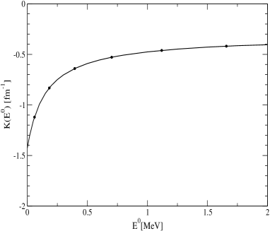
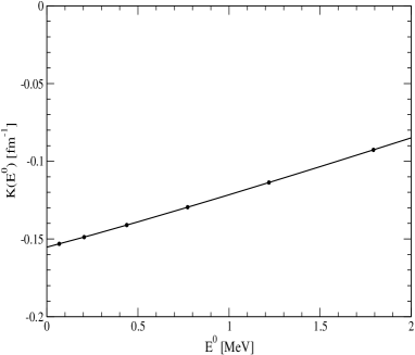
Figure 1: The $n-d$ effective range function for $J=1/2^{+}$ (left panel) and $J=3/2^{+}$ (right panel). The solid points are obtained from the second order estimates using the integral relations with bound state like wave functions at the corresponding energies.

3 Analysis of Three Nucleon Force Models

In order to reproduce correctly the three-nucleon bound state energy, different three-nucleon force (TNF) models have been constructed during the past years as the Tucson-Melbourne (TM), Brazil (BR) and the Urbana IX (URIX) models [12, 13, 14]. These models are based on the exchange mechanism of two pions between three nucleons. More recently, TNFs have been derived [15] using a chiral effective field theory at next-to-next-to-leading order. A local version of these interactions (hereafter referred as N2LOL) can be found in Ref. [16]. At next-to-next-to-leading order, the TNF has two unknown constants that have to be determined. It is a common practice to determine these parameters from the three- and four-nucleon binding energies ($B$(³H) and $B$(⁴He), respectively).

The $n-d$ doublet scattering length ${}^{2}a_{nd}$ is correlated, to some extent, to the $A=3$ binding energy through the so-called Phillips line [17, 18]. However the presence of TNFs could break this correlation. Therefore ${}^{2}a_{nd}$ can be used as an independent observable to evaluate the capability of the interaction models to describe the low energy region. In Ref. [19] results for different combinations of NN interactions plus TNF models are given. These results are shown for the quantities of interest in Table I and are compared to the experimental values of the binding energies and ${}^{2}a_{nd}$ [20]. From the table, we can observe that the models are not able to describe simultaneously the $A=3,4$ binding energies and ${}^{2}a_{nd}$.

Table 1: The triton and ⁴He binding energies $B$ (MeV), and doublet scattering length ${}^{2}a_{nd}$ (fm) calculated using the AV18 and the N3LO-Idaho two-nucleon potentials, and the AV18+URIX, AV18+TM’ and N3LO-Idaho+N2LOL two- and three-nucleon interactions. The experimental values are given in the last row.

Potential	$B$(3H)	$B$(4He)	${}^{2}a_{nd}$
AV18	7.624	24.22	1.258
N3LO-Idaho	7.854	25.38	1.100
AV18+TM’	8.440	28.31	0.623
AV18+URIX	8.479	28.48	0.578
N3LO-Idaho+N2LOL	8.474	28.37	0.675
Exp.	8.482	28.30	0.645$\pm$0.003$\pm$0.007

In Ref. [3] a comparative study of the aforementioned TNF models has been performed. Let us briefly review their structure. From the general form

$$W=\sum_{i<j<k}W(i,j,k)\;\;,$$ (7)

a generic term can be decomposed as

$$W(1,2,3)=aW_{a}(1,2,3)+bW_{b}(1,2,3)+dW_{d}(1,2,3)+c_{D}W_{D}(1,2,3)+c_{E}W_{E}(1,2,3)\;.$$ (8)

Each term corresponds to a different mechanism and has a different operatorial structure. The specific form of these terms in configuration space is:

$$W_{a}(1,2,3)=W_{0}(\bm{\tau}_{1}\cdot\bm{\tau}_{2})(\bm{\sigma}_{1}\cdot\bm{r}_{31})(\bm{\sigma}_{2}\cdot\bm{r}_{23})y(r_{31})y(r_{23})$$ (9)

$$W_{b}(1,2,3)=W_{0}(\bm{\tau}_{1}\cdot\bm{\tau}_{2})[(\bm{\sigma}_{1}\cdot\bm{\sigma}_{2})y(r_{31})y(r_{23})$$

$$\hskip 56.9055pt+(\bm{\sigma}_{1}\cdot\bm{r}_{31})(\bm{\sigma}_{2}\cdot\bm{r}_{23})(\bm{r}_{31}\cdot\bm{r}_{23})t(r_{31})t(r_{23})$$

$$\hskip 56.9055pt+(\bm{\sigma}_{1}\cdot\bm{r}_{31})(\bm{\sigma}_{2}\cdot\bm{r}_{31})t(r_{31})y(r_{23})$$

$$\hskip 56.9055pt+(\bm{\sigma}_{1}\cdot\bm{r}_{23})(\bm{\sigma}_{2}\cdot\bm{r}_{23})y(r_{31})t(r_{23})]$$

$$W_{d}(1,2,3)=W_{0}(\bm{\tau}_{3}\cdot\bm{\tau}_{1}\times\bm{\tau}_{2})[(\bm{\sigma}_{3}\cdot\bm{\sigma}_{2}\times\bm{\sigma}_{1})y(r_{31})y(r_{23})$$

$$\hskip 56.9055pt+(\bm{\sigma}_{1}\cdot\bm{r}_{31})(\bm{\sigma}_{2}\cdot\bm{r}_{23})(\bm{\sigma}_{3}\cdot\bm{r}_{31}\times\bm{r}_{23})t(r_{31})t(r_{23})$$

$$\hskip 56.9055pt+(\bm{\sigma}_{1}\cdot\bm{r}_{31})(\bm{\sigma}_{2}\cdot\bm{r}_{31}\times\bm{\sigma}_{3})t(r_{31})y(r_{23})$$

$$\hskip 56.9055pt+(\bm{\sigma}_{2}\cdot\bm{r}_{23})(\bm{\sigma}_{3}\cdot\bm{r}_{23}\times\bm{\sigma}_{1})y(r_{31})t(r_{23})]\;\;,$$

with $W_{0}$ an overall strength. The $b$- and $d$-terms are present in the three models whereas the $a$-term is present in the TM’ and N2LOL and not in URIX. The last two terms in Eq.(8) correspond to a two-nucleon (2N) contact term with a pion emitted or absorbed ($D$-term) and to a three-nucleon (3N) contact interaction ($E$-term). Their local form, derived in Ref. [16], is

$$W_{D}(1,2,3)=W_{0}^{D}(\bm{\tau}_{1}\cdot\bm{\tau}_{2})\{(\bm{\sigma}_{1}\cdot\bm{\sigma}_{2})[y(r_{31})Z_{0}(r_{23})+Z_{0}(r_{31})y(r_{23})]$$ (10)

$$\hskip 56.9055pt+(\bm{\sigma}_{1}\cdot\bm{r}_{31})(\bm{\sigma}_{2}\cdot\bm{r}_{31})t(r_{31})Z_{0}(r_{23})$$

$$\hskip 56.9055pt+(\bm{\sigma}_{1}\cdot\bm{r}_{23})(\bm{\sigma}_{2}\cdot\bm{r}_{23})Z_{0}(r_{31})t(r_{23})\}$$

$$W_{E}(1,2,3)=W_{0}^{E}(\bm{\tau}_{1}\cdot\bm{\tau}_{2})Z_{0}(r_{31})Z_{0}(r_{23})\,\,.$$

The constants $W_{0}^{D}$ and $W_{0}^{E}$ fix the strength of these terms. In the case of the URIX model the $D$-term is absent whereas the $E$-term is present without the isospin operatorial structure and it has been included as purely phenomenological, without justifying its form from a particular exchange mechanism. The different form for the profile functions of each model, $y(r)$, $t(r)$ and $Z_{0}(r)$ are given in Ref. [3]. In that reference the strengths relative to the different terms have been varied in order to reproduce, as close as possible, $B$(³H) and $B$(⁴He) and ${}^{2}a_{nd}$. With these new parametrizations selected polarization observables can been calculated and compared to the experimental data. In particular using the N2LOL three-nucleon force a small improvement in the description of the vector analyzing powers $A_{y}$ and $iT_{11}$ at low energies has been obtained. This is shown in Fig. 2 in which the predictions for $p-d$ $A_{y}$ and $d-p$ $iT_{11}$ at $E_{p}=3$ MeV of the AV18+N2LOL model (grey band) is compared to those ones of the AV18+UR model (solid line). From the figure we can observed that the discrepancy has been appreciable reduced.

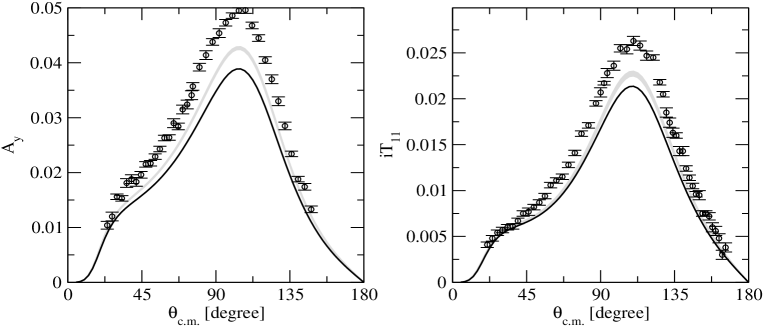
Figure 2: The $p-d$ analyzing powers $A_{y}$ and $iT_{11}$ at $E_{p}=3$ MeV for the AV18+N2LOL (grey band) and AV18+UR (solid line) models. Experimental data are from Ref. [21].

The effects of the N2LOL TNF is much more evident in the four nucleon system. In fact, in Fig. 3 the $p-^{3}$He analyzing power $A_{y}$ is shown at three energies using the N3LO-Idaho NN interaction plus the N2LOL TNF (dashed line) and the AV18+UR model (solid line). We can see the big effect produced by the inclusion of the N2LOL TNF model. It should be noticed that the observable calculated using the N3LO-Idaho or the AV18 NN forces alone results close to the predictions of the AV18+UR model (see Ref. [22]), indicating that the improvement is given by the inclusion of the N2LOL force. As in the three-nucleon system, this TNF model considerable reduces the discrepancy obtained in the description of this observable.

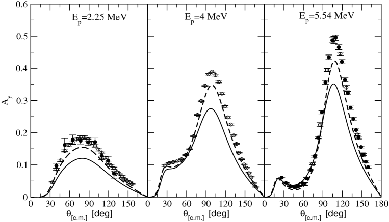
Figure 3: The $p-^{3}$He analyzing powers $A_{y}$ at three energies for the N3LO-Idaho+N2LOL (dashed line) and AV18+UR (solid line) models. Experimental data are from Refs. [23, 24].

4 Conclusions

Two different aspects of the description of few-nucleon systems have been discussed. Firstly, scattering states below the deuteron breakup threshold has been calculated using bound state like wave functions. The starting point in this analysis was the integral relations recently derived from the KVP. Finally an analysis of the effects of TNF models has been briefly discussed in the vector analyzing powers in $p-d$ and $p-^{3}$He scattering. In particular it was shown that the inclusion of the N2LOL TNF appreciable improves the description of those observables. Further studies on these subjects are at present in progress.

The results presented in this work have been obtained in collaboration with C. Romero-Redondo and E. Garrido (CSIC), P. Barletta (UCL) and my colleagues in Pisa, M. Viviani, L. Girlanda and L.E. Marcucci.

References

- [1] A. Kievsky, M. Viviani, and S. Rosati, Polarization observables in p-d scattering below 30 MeV, Phys. Rev. C 64, 024002 (2001)
- [2] B.M. Fisher et al., Proton-3He elastic scattering at low energies, Phys. Rev. C 74, 034001 (2006)
- [3] A. Kievsky, M. Viviani, L. Girlanda and L.E. Marcucci, Comparative study of three-nucleon force models in A=3,4 systems, Phys. Rev. C 81, 044003 (2010)
- [4] A. Kievsky et al., Benchmark calculations for polarization observables in three-nucleon scattering, Phys. Rev. C58, 3085 (1998)
- [5] R. Lazauskas et al., Low energy n-3H scattering: a novel testground for nuclear interaction, Phys. Rev. C71, 064003 (2005)
- [6] S.C. Pieper, K. Varga, and R.B. Wiringa, Quantum Monte Carlo calculations of A=9,10 nuclei, Phys. Rev. C66, 044310 (2002)
- [7] P. Navrátil et al., Structure of Nuclei with Two- Plus Three-Nucleon Interactions from Chiral Effective Field Theory, Phys. Rev. Lett. 99, 042501 (2007)
- [8] Y. Suzuki, W. Horiuchi, and K. Arai, Phase-shift calculation using continuum-discretized states, Nucl. Phys. A823, 1 (2009)
- [9] A. Kievsky et al., Variational description of continuum states in terms of integral relations, Phys. Rev. C81, 034002 (2010)
- [10] P. Barletta et al., Integral relations for three-body continuum states with the adiabatic expansion, Phys. Rev. Lett. 103, 090402 (2009)
- [11] R.A Malfliet and J.A. Tjon, Solution of the Faddeev equations for the triton problem using local two-particle interactions, Nucl. Phys. A127, 161 (1969)
- [12] S.A. Coon and W. Glöckle, Two-pion-exchange three-nucleon potential: Partial wave analysis in momentum space, Phys. Rev. C 23, 1790 (1981)
- [13] H.T. Coelho, T.K. Das, and M.R. Robilotta, Two-pion-exchange three-nucleon force and the 3H and 3He nuclei, Phys. Rev. C 28, 1812 (1983);
- [14] B.S. Pudliner, V. R. Pandharipande, J. Carlson, and R.B. Wiringa, Quantum Monte Carlo Calculations of Nuclei, Phys. Rev. Lett. 74, 4396 (1995)
- [15] E. Epelbaum et al., Three-nucleon forces from chiral effective field theory, Phys. Rev. C 66, 064001 (2002)
- [16] P. Navratil, Local three-nucleon interaction from chiral effective field theory, Few-Body Syst. 41, 117 (2007)
- [17] A.C. Phillips, Consistency of the low-energy three-nucleon observables and the separable interaction model, Nucl. Phys. A 107, 209 (1968)
- [18] P.F. Bedaque, H.-W. Hammer, and U. van Kolck, The three-boson system with short-range interactions, Nucl. Phys. A 646, 444 (1999)
- [19] A. Kievsky et al., A high-precision variational approach to three- and four-nucleon bound and zero-energy scattering states, J. Phys. G: Nucl. Part. Phys. 35, 063101 (2008)
- [20] K. Schoen et al., Precision neutron interferometric measurements and updated evaluations of the n-p and n-d coherent neutron scattering lengths, Phys. Rev. C 67, 044005 (2003)
- [21] S. Shimizu et al., Analyzing powers of p+d scattering below the deuteron breakup threshold, Phys. Rev. C 52, 1193 (1995)
- [22] M. Viviani et al., Proton-3He elastic scattering at low energies and the “ Puzzle”, EPJ Web of Conferences 3, 05012 (2010)
- [23] M.T. Alley and L.D. Knutson, Effective range parametrization of phase shifts for He elastic scattering between and MeV, Phys. Rev. C 48, 1901 (1993)
- [24] T. V. Daniels et al., Spin-correlation coefficients and phase-shift analysis for He elastic scattering, Phys. Rev. C 82, 034002 (2010)