subject
Parallel Online Learning
1 Online Learning
One well-known general approach to machine learning is to repeatedly greedily update a partially learned system using a single labeled data instance. A canonical example of this is provided by the perceptron algorithm (Rosenblatt,, 1958) which modifies a weight vector by adding or subtracting the features of a misclassified instance. More generally, typical methods compute the gradient of the prediction’s loss with respect to the weight vector’s parameters, and then update the system according to the negative gradient. This basic approach has many variations and extensions, as well as at least two names. In the neural network literature, this approach is often called “stochastic gradient descent” , while in the learning theory literature it is typically called “online gradient descent”. For the training of complex nonlinear prediction systems, the stochastic gradient descent approach was described long ago and has been standard practice for at least two decades (Bryson and Ho,, 1969; Rumelhart et al.,, 1986; Amari,, 1967).
Algorithm 1 describes the basic gradient descent algorithm we consider here. The core algorithm uses a differentiable loss function to measure the quality of a prediction with respect to a correct prediction , and a sequence of learning rates . Qualitatively, a “learning rate” is the degree to which the weight parameters are adjusted to predict in accordance with a data instance. For example, a common choice is squared loss where and a common learning rate sequence is .
There are several basic observations regarding efficiency of online learning approaches. {itemize*}
At a high level, many learning system make a sequence of greedy improvements. For such systems, it is difficult to reduce these improvements to one or just a few steps of greedy improvement, simply because the gradient provides local information relevant only to closely similar parameterizations, while successful prediction is a global property. This observation applies to higher order gradient information such as second derivatives as well. An implication of this observation is that multiple steps must be taken, and the most efficient way to make multiple steps is to take a step after each instance is observed.
If the same instance occurs twice in the data, it’s useful to take advantage of data as it arrives. Take the extreme case where every instance is replicated times. Here an optimization algorithm using fractions of of the data at a time would enjoy an -fold speedup relative to an algorithm using full views of the data for optimization. While in practice it is difficult to ascertain these properties beforehand, it is highly desirable to have algorithms which can take advantage of redundancy and similarity as data arrives.
The process of taking a gradient step is generally amortized by prediction itself. For instance, with the square loss , the gradient is given by for , so the additional cost of the gradient step over the prediction is roughly just a single multiply and store per feature. Similar amortization can also be achieved with complex nonlinear circuit-based functions, for instance, when they are compositions of linear predictors.
The process of prediction can often be represented in vectorial form such that highly optimized linear algebra routines can be applied to yield an additional performance improvement.
Both the practice of machine learning and the basic observations above suggest that gradient descent learning techniques are well suited to address large scale machine learning problems. Indeed, the techniques are so effective, and modern computers are so fast, that we might imagine no challenge remains. After all, a modern computer might have 8 cores operating at 3GHz, each core capable of floating point operations per clock cycle, providing a peak performance of 96GFlops. A large dataset by today’s standards is about webscale, perhaps instances, each features in size. Taking the ratio, this suggests that a well-implemented learning algorithm might be able to process such a dataset in under 20 minutes. Taking into account that GPUs are capable of delivering at least one order of magnitude more computation and that FPGAs might provide another order of magnitude, this suggests no serious effort should be required to scale up learning algorithms, at least for simple linear predictors.
However, considering only floating point performance is insufficient to capture the constraints imposed by real systems: the limiting factor is not computation, but rather network limits on bandwidth and latency. This chapter is about dealing with these limits in the context of gradient descent learning algorithms. We take as our baseline gradient descent learning algorithm a simple linear predictor, which we typically train to minimize squared loss. Nevertheless, we believe our findings with respect to these limitations qualitatively apply to many other learning algorithms operating according to gradient descent on large datasets.
Another substantial limit is imposed by label information—it’s difficult in general to cover the cost of labeling instances. For large datasets relevant to this work, it’s typically the case that label information is derived in some automated fashion—for example a canonical case is web advertisement where we might have advertisements displayed per day, of which some are clicked on and some are not.
2 Limits due to Bandwidth and Latency
The bandwidth limit is well-illustrated by the Stochastic Gradient Descent (SGD) implementation (Bottou,, 2008). Leon Bottou released it as a reference implementation along with a classification problem with 781K instances and 60M total (non-unique) features derived from RCV1 (Lewis et al.,, 2004). On this dataset, the SGD implementation might take 20 seconds to load the dataset into memory and then learn a strong predictor in 0.4 seconds. This illustrates that the process of loading the data from disk at 15MB/s is clearly the core bottleneck.
But even if that bottleneck were removed we would still be far from peak performance: 0.4 seconds is about 100 times longer than expected given the peak computational limits of a modern CPU. A substantial part of this slowdown is due to the nature of the data, which is sparse. With sparse features, each feature might incur the latency to access either cache or RAM (typically a 10x penalty), imposing many-cycle slowdowns on the computation. Thus, performance is sharply limited by bandwidth and latency constraints which in combination slow down learning substantially.
Luckily, gradient descent style algorithms do not require loading all data into memory. Instead one data instance can be loaded, a model updated, and then the instance discarded. A basic question is: Can this be done rapidly enough to be an effective strategy? For example, a very reasonable fear is that the process of loading and processing instances one at a time induces too much latency, slowing the overall approach unacceptably.
The Vowpal Wabbit (VW) software (Langford et al.,, 2007) provides an existence proof that it is possible to have a fast fully online implementation which loads data as it learns. On the dataset above, VW can load and learn on the data simultaneously in about 3 seconds, an order of magnitude faster than SGD. A number of tricks are required to achieve this, including a good choice of cache format, asynchronous parsing, and pipelining of the computation. A very substantial side benefit of this style of learning is that we are no longer limited to datasets which fit into memory. A dataset can be either streamed from disk or over the network, implying that the primary bottleneck is bandwidth, and the learning algorithm can handle datasets with perhaps non-unique features in a few hours.
The large discrepancy between bandwidth and available computation suggests that it should be possible to go beyond simple linear models without a significant computational penalty: we can compute nonlinear features of the data and build an extended linear model based on those features. For instance, we may use the random kitchen sink features (Rahimi and Recht,, 2008) to obtain prediction performance comparable with Gaussian RBF kernel classes. Furthermore, while general polynomial features are computationally infeasible it is possible to obtain features based on the outer product of two sets of features efficiently by explicitly expanding such features on the fly. These outer product features can model interaction between two sources of information, for example the interaction of (query,result) feature pairs is often relevant in internet search settings.
VW allows the implicit specification of these outer product features via specification of the elements of the pairs. The outer product features thus need not be read from disk, implying that the disk bandwidth limit is not imposed. Instead, a new limit arises based on random memory access latency and to a lesser extent on bandwidth constraints. This allows us to perform computation in a space of up to features with a throughput in the order of features/second. Note that VW can additionally reduce the dimensionality of each instance using feature hashing (Shi et al.,, 2009; Weinberger et al.,, 2009) , which is essential when the (expanded) feature space is large, perhaps even exceeding memory size. The core idea here is to use a hash function which sometimes collides features. The learning algorithm learns to deal with these collisions, and the overall learning and evaluation process happens much more efficiently due to substantial space savings.
This quantity remains up to two orders of magnitude below the processing limit imposed by a modern CPU (we have up to 100 Flops available per random memory access). This means that there is plenty of room to use more sophisticated learning algorithms without substantially slowing the learning process. Nevertheless, it also remains well below the size of the largest datasets, implying that our pursuit of a very fast efficient algorithm is not yet complete.
To make matters more concrete assume we have datasets of 10TB size (which is not uncommon for web applications). If we were to stream this data from disk we cannot expect a data stream of more than 100MB/s per disk (high performance arrays might achieve up to 5x this throughput, albeit often at a significant CPU utilization). This implies that we need to wait at least seconds, i.e. 30 hours to process this data on a single computer. This is assuming an optimal learning algorithm which needs to see each instance only once and a storage subsystem which is capable of delivering sustained peak performance for over a day. Even with these unrealistic assumptions this is often too slow.
3 Parallelization Strategies
Creating an online algorithm to process large amounts of data directly limits the designs possible. In particular, it suggests decomposition of the data either in terms of instances or in terms of features as depicted in Figure 1. Decomposition in terms of instances automatically reduces the load per computer since we only need to process and store a fraction of the data on each computer. We refer to this partitioning as “instance sharding”111In the context of data, “shard” is typically used to define a partition without any particular structure other than size..
An alternative is to decompose data in terms of its features. While it does not reduce the number of instances per computer, it reduces the data per computer by reducing the number of features associated with an instance for each computer, thus increasing the potential throughput per computer.
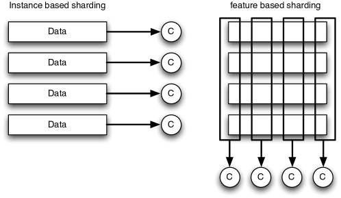
A typical instance shard scheme runs the learning algorithm on each shard, combines the results in some manner, and then runs a learning algorithm again (perhaps with a different initialization) on each piece of the data. An extreme case of the instance shard approach is given by parallelizing statistical query algorithms (Chu et al.,, 2007), which compute statistics for various queries over the entire dataset, and then update the learned model based on these queries, but there are many other variants as well (Mann et al.,, 2009; McDonald et al.,, 2010). The instance shard approach has a great virtue—it’s straightforward and easy to program.
A basic limitation of the instance shard approach is the “combination” operation which does not scale well with model complexity. When a predictor is iteratively built based on statistics, it is easy enough to derive an aggregate statistic. When we use an online linear predictor for each instance shard, some averaging or weighted averaging style of operation is provably sensible. However, when a nonlinear predictor is learned, it is unclear how to combine the results. Indeed, when a nonlinear predictor has symmetries, and the symmetries are broken differently on different instance shards, a simple averaging approach might cancel the learning away. An example of a symmetry is provided by a two-layer neural network with 2 hidden nodes. By swapping the weights in the first hidden node with the weights of the second hidden node, and similarly swapping the weights in the output node we can build a representationally different predictor with identical predictions. If these two neural networks then have their weights averaged, the resulting predictor can perform very poorly.
We have found a feature shard approach more effective after the (admittedly substantial) complexity of programming has been addressed. The essential idea in a feature shard approach is that a learning algorithm runs on a subset of the features of each instance, then the predictions on each shard are combined to make an overall prediction for each instance. In effect, the parameters of the global model are partitioned over different machines. One simple reason why the feature shard approach works well is due to caching effects—any learned model is distributed across multiple nodes and hence better fits into the cache of each node. This combination process can be a simple addition, or the predictions from each shard can be used as features for a final prediction process, or the combination could even be carried out in a hierarchical fashion. After a prediction is made, a gradient based update can be made to weights at each node in the process. Since we are concerned with datasets less than in size, the bandwidth required to pass a few bytes per instance around is not prohibitive.
One inevitable side effect of either the instance shard or the feature shard approach is a delayed update, as explained below. Let be the number of instances and be the number of computation nodes. In the instance shard approach the delay factor is equal to , because updates can occur before information from a previously seen instance is incorporated into the model. With the feature shard approach, the latency is generally smaller, but more dependent on the network architecture. In the asymptotic limit when keeping the bandwidth requirements of all nodes constant, the latency grows as when the nodes are arranged in a binary tree hierarchy; in this case, the prediction and gradient computations are distributed in a divide-and-conquer fashion and is completed in time proportional to the depth of the recursion, which is . In the current implementation of VW, a maximum latency of instances is allowed. It turns out that any delay can degrade performance substantially, at least when instances arrive adversarially, as we outline next.
4 Delayed Update Analysis
We have argued that both instance sharding and feature sharding approaches require delayed updates in a parallel environment. Here we state some analysis of the impact of delay, as given by the delayed gradient descent algorithm in Algorithm 2. We assume that at time we observe some instance with associated label . Given the instance we generate some prediction . Based on this we incur a loss such as .
Given this unified representation we consider the following optimization algorithm template. It differs from Algorithm 1 because the update is delayed by rounds. This aspect models the delay due to the parallelization strategy for implementing the gradient descent computation.
4.1 Guarantees
We focus on the impact of delay on the convergence rate of the weight vector learned by the algorithm. Convergence rate is a natural performance criterion for online learning algorithms, as it characterizes the trade-off between running time and learning accuracy (measured specifically in number of instances versus error rate).
Introducing delay between data presentation and updates can lead to a substantial increase in error rate. Consider the case where we have a delay of between the time we see an instance and when we are able to update based on the instance. If we are shown duplicates of the same data, i.e. in sequence we have no chance of responding to in time and the algorithm cannot converge to the best weight vector any faster than times the rate of an algorithm which is able to respond instantly. Note that this holds even if we are told beforehand that we will see the same instance times.
This simple reasoning shows that for an adversarially chosen sequence of instances the regret (defined below) induced by a delay of can never be better than that of the equivalent no-delay algorithm whose convergence speed is reduced by a factor of . It turns out that these are the very rates we are able to obtain in the adversarial setting. On the other hand, in the non-adversarial setting, we are able to obtain rates which match those of no-delay algorithms, albeit with a sizable additive constant which depends on the delay.
The guarantees we provide are formulated in terms of a regret, i.e. as a discrepancy relative to the best possible solution defined with knowledge of all events. Formally, we measure the performance of the algorithm in terms of
| (1) | ||||
Theorem 1 (Worst case guarantees for delayed updates; Langford et al.,, 2009).
If and the norms of the gradients are bounded by , then
| (2) |
when we choose the learning rate . If, in addition, is strongly convex with modulus of convexity we obtain the guarantee
with learning rate , where is a function independent of .
In other words the average error of the algorithm (as normalized by the number of seen instances) converges at rate whenever the loss gradients are bounded and at rate whenever the loss function is strongly convex. This is exactly what we would expect in the worst case: an adversary may reorder instances so as to maximally slow down progress. In this case a parallel algorithm is no faster than a sequential code. While such extreme cases hardly occur in practice, we have observed experimentally that for sequentially correlated instances, delays can rapidly degrade learning.
If subsequent instances are only weakly correlated or IID, it is possible to prove tighter bounds where the delay does not directly harm the update (Langford et al.,, 2009). The basic structure of these bounds is that they have a large delay-dependent initial regret after which the optimization essentially degenerates into an averaging process for which delay is immaterial. These bounds have many details, but a very crude alternate form of analysis can be done using sample complexity bounds. In particular, if we have a set of predictors and at each timestep choose the best predictor on the first timesteps, we can bound the regret to the best predictor according to the following:
Theorem 2 (IID Case for delayed updates).
If all losses are in , for all IID data distributions over features and labels, for any in , with probability
| (3) |
Proof.
The proof is a straightforward application of the Hoeffding bound. At every timestep , we have labeled data instances. Applying the Hoeffding bound for every hypothesis , we have that with probability , . Applying a union bound over all hypotheses and timesteps implies the same holds with probability at least . The algorithm which chooses the best predictor in hindsight therefore chooses a predictor with expected loss at most worse than the best. Summing over timesteps, we get: . This is a bound on an expected regret. To get a bound on the actual regret, we can simply apply a Hoeffding bound again yielding the theorem result. ∎
5 Parallel Learning Algorithms
We have argued that delay is generally bad when doing online learning (at least in an adversarial setting), and that it is also unavoidable when parallelizing. This places us in a bind: How can we create an effective parallel online learning algorithm? We’ll discuss two approaches based on multicore and multinode parallelism.
5.1 Multicore Feature Sharding
A multicore processor consists of multiple CPUs which operate asynchronously in a shared memory space. It should be understood that because multicore parallelization does not address the primary bandwidth bottleneck, its usefulness is effectively limited to those datasets and learning algorithms which require substantial computation per raw instance used. In the current implementation, this implies the use of feature pairing, but there are many learning algorithms more complex than linear prediction where this trait may also hold.
The first version of Vowpal Wabbit used an instance sharding approach for multicore learning, where the set of weights and the instance source was shared between multiple identical threads which each parsed the instance, made a prediction, and then did an update to the weights. This approach was effective for two threads yielding a near factor-of-2 speedup since parsing of instances required substantial work. However, experiments with more threads on more cores yielded no further speedups due to lock contention. Before moving on to a feature sharding approach, we also experimented with a dangerous parallel programming technique: running with multiple threads that do not lock the weight vector. This did yield improved speed, but at a cost in reduced learning rate and nondeterminism which was unacceptable.
The current implementation of Vowpal Wabbit uses an asynchronous parsing thread which prepares instances into just the right format for learning threads, each of which computes a sparse-dense vector product on a disjoint subset of the features. The last thread completing this sparse-dense vector product adds together the results and computes an update which is then sent to all learning threads to update their weights, and then the process repeats. Aside from index definition related to the core hashing representation (Shi et al.,, 2009; Weinberger et al.,, 2009) Vowpal Wabbit employs, the resulting algorithm is identical to the single thread implementation. It should be noted that although processing of instances is fully synchronous there is a small amount of nondeterminism between runs due to order-of-addition ambiguities between threads. In all our tests, this method of multicore parallelization yielded virtually identical prediction performance with negligible overhead compared to non-threaded code and sometimes substantial speedups. For example, with 4 learning threads, about a factor of 3 speedup is observed.
We anticipate that this approach to multicore parallelization will not scale to large numbers of cores, because the very tight coupling of parallelization requires low latency between the different cores. Instead, we believe that multinode parallelization techniques will ultimately need to be used for multicore parallelization, motivating the next section.
5.2 Multinode Feature Sharding
The primary distinction between multicore and multinode parallelization is latency, with the latency between nodes many orders of magnitude larger than for cores. In particular, the latency between nodes is commonly much larger than the time to process an individual instance, implying that any per-instance blocking operation, as was used for multicore parallelization, is unacceptable.
This latency also implies a many-instance delayed update which, as we have argued, incurs a risk of substantially degrading performance. In an experiment to avoid this risk, we investigated the use of updates based on information available to only one node in the computation, where there is no delay. Somewhat surprisingly, this worked better than our original predictor.
5.2.1 Tree Architectures
Our strategy is to employ feature sharding across several nodes, each of which updates its parameters online as a single-node learning algorithm would. So, ignoring the overhead due to creating and distributing the feature shards (which can be minimized by reorganizing the dataset), we have so far fully decoupled the computation. The issue now is that we have independent predictors each using just a subset of the features (where is the number of feature shards), rather than a single predictor utilizing all of the features. We reconcile this in the following manner: (i) we require that each of these nodes compute and transmit a prediction to a master node after receiving each new instance (but before updating its parameters); and (ii) we use the master node to treat these predictions as features, from which the master node learns to predict the label in an otherwise symmetric manner. Note that the master node must also receive the label corresponding to each instance, but this can be handled in various ways with minimal overhead (e.g., it can be piggybacked with one of the subordinate node’s predictions). The end result, illustrated in Figure 2, is a two-layer architecture for online learning with reduced latency at each node and no delay in parameter updates.
Naturally, the strategy described above can be iterated to create multi-layered architectures that further reduce the latency at each node. At the extreme, the architecture becomes a (full) binary tree: each leaf node (at the bottom layer) predicts using just a single feature, and each internal node predicts using the predictions of two subordinate nodes in the next lower layer as features (see Figure 3). Note that each internal node may incur delay proportional to its fan-in (in-degree), so reducing fan-in is desirable; however, this comes at the cost of increased depth and thus prediction latency. Therefore, in practice the actual architecture that is deployed may be somewhere in between the binary tree and the two-layer scheme. Nevertheless, we will study the binary tree structure further because it illustrates the distinctions relative to a simple linear prediction architecture.
5.2.2 Convergence Time vs Representation Power
The price of the speed-up that comes with the no-delay approach (even with the two-layer architecture) is paid in representation power. That is, the no-delay approach learns restricted forms of linear predictors relative to what can be learned by ordinary (delayed) gradient descent. To illustrate this, we compare the resulting predictors from the no-delay approach with the binary tree architecture and the single-node linear architecture. Let be a random vector (note that the subscripts now index the features) and be a random variable. Gradient descent using a linear architecture converges toward the least-squares linear predictor of from , i.e.,
where
in time roughly linear in the number of features (Kivinen and Warmuth,, 1995).
The gradient descent strategy with the binary tree architecture, on the other hand, learns weights locally at each node; the weights at each node therefore converge to weights that are locally optimal for the input features supplied to the node. The final predictor is linear in the input features but can differ from the least-squares solution. To see this, note first that the leaf nodes learn weights , where
Then, the th layer of nodes learns weights from the predictions of the th layer; recursively, a node whose input features are the predictions of the th and th nodes from layer learns the weights . By induction, the prediction of the th node in layer is linear in the subset of variables that are descendants of this node in the binary tree. Let denote these weights and denote the corresponding feature vector. Then can be expressed as
where and . Then, the prediction at this particular node in layer is
which is linear in . Therefore, the overall prediction is linear in , with the weight attached to being a product of weights at the different levels. However, these weights can differ significantly from when the features are highly correlated, as the tree architecture only ever considers correlations between (say) and through the scalar summary . Thus, the representational expressiveness of the binary tree architecture is constrained by the local training strategy.
The tree predictor can represent solutions with complexities between Naïve Bayes and a linear predictor. Naïve Bayes learns weights identical to the bottom layer of the binary tree, but stops there and combines the individual predictions with a trivial sum: . The advantage of Naïve Bayes is its convergence time: because the weights are learned independently, a union bound argument implies convergence in just time, which is exponentially faster than the convergence time using the linear architecture!
The convergence time of gradient descent with the binary tree architecture is roughly . To see this, note that the th layer converges in roughly time since there are parameters that need to converge, plus the time for the th layer to converge. Inductively, this is . Thus, all of the weights have converged by the time the final layer () converges; this gives an overall convergence time of . This is slightly slower than Naïve Bayes, but still significantly faster than the single-node linear architecture.
The advantage of the binary tree architecture over Naïve Bayes is that it can account for variability in the prediction power of various feature shards, as the following result demonstrates.
Proposition 3.
There exists a data distribution for which the binary tree architecture can represent the least-squares linear predictor but Naïve Bayes cannot.
Proof.
Suppose the data comes from a uniform distribution over the following four points:
| Point 1 | ||||
|---|---|---|---|---|
| Point 2 | ||||
| Point 3 | ||||
| Point 4 |
Naïve Bayes yields the weights , which incurs mean squared-error . On the other hand, gradient descent with the binary tree architecture learns additional weights:
which ultimately yields an overall weight vector of
which has zero mean squared-error. ∎
In the proof example, the features are, individually, equally correlated with the label . However, the feature is correlated with the two individually uncorrelated features and , but Naïve Bayes is unable to discover this whereas the binary tree architecture can compensate for it.
Of course, as mentioned before, the binary tree architecture (and Naïve Bayes) is weaker than the single-node linear architecture in expressive power due to its limited accounting of feature correlation.
Proposition 4.
There exists a data distribution for which neither the binary tree architecture nor Naïve Bayes can represent the least-squares linear predictor.
Proof.
Suppose the data comes from a uniform distribution over following four points:
| Point 1 | ||||
|---|---|---|---|---|
| Point 2 | ||||
| Point 3 | ||||
| Point 4 |
The optimal least-squares linear predictor is the all-ones vector and incurs zero squared-error (since for every point). However, both Naïve Bayes and the binary tree architecture yield weight vectors in which zero weight is assigned to , since is uncorrelated with ; any linear predictor that assigns zero weight to has expected squared-error at least . ∎
5.3 Experiments
Here, we detail experimental results conducted on a medium size proprietary ad display dataset. The task associated with the dataset is to derive a good policy for choosing an ad given user, ad, and page display features. This is accomplished via pairwise training concerning which of two ads was clicked on and element-wise evaluation with an offline policy evaluator (Langford et al.,, 2008). There are several ways to measure the size of this dataset—it is about 100Gbytes when gzip compressed, has around 10M instances, and about 125G non-unique nonzero features. In the experiments, VW was run with weights, which is substantially smaller than the number of unique features. This discrepancy is accounted for by the use of a hashing function, with being chosen because it is large enough such that a larger numbers of weights do not substantially improve results.
In the experimental results, we report the ratio of progressive validation squared losses (Blum et al.,, 1999) and wall clock times to a multicore parallelized version of Vowpal Wabbit running on the same data and the same machines. Here, the progressive validation squared loss is the average over of where critically, is the prediction just prior to an update. When data is independent, this metric has deviations similar to the average loss computed on held-out evaluation data.
Every node has 8 CPU cores and is connected via gigabit Ethernet. All learning results are obtained with single pass learning on the dataset using learning parameters optimized to control progressive validation loss. The precise variant of the multinode architecture we experimented with is detailed in Figure 4. In particular, note that we worked with a flat hierarchy using 1-8 feature shards (internal nodes). All code is available in the current Vowpal Wabbit open source code release.
a)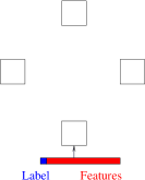 b)
b)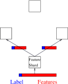 c)
c)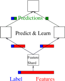 d)
d)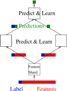
 |
 |
| (a) | (b) |
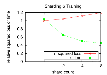
Results are reported in Figure 5. The first thing to note in Figure 5(a) is that there is essentially no loss in time and precisely no loss in solution quality for using two machines (shard count ): one for a no-op shard (used just for sending data to the other nodes) and the other for learning. We also note that the running time does not decrease linearly in the number of shards, which is easily explained by saturation of the network by the no-op sharding node. Luckily, this is not a real bottleneck, because the process of sharding instances is stateless and (hence) completely parallelizable. As expected, the average solution quality across feature shards also clearly degrades with the shard count. This is because the increase in shard count implies a decrease in the number of features per nodes, which means each node is able to use less information on which to base its predictions.
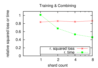
Upon examination of Figure 5(b), we encounter a major surprise—the quality of the final solution substantially improves over the single node solution since the relative squared loss is less than . We have carefully verified this. It is most stark when there is only one feature shard, where we know that the solution on that shard is identical to the single node solution. This output prediction is then thresholded to the interval (as the labels are either or ) and passed to a final prediction node which uses the prediction as a feature and one (default) constant feature to make a final prediction. This very simple final prediction step is where the large improvement in prediction quality occurs. Essentially, because there are only two features (one is constant!), the final output node performs a very careful calibration which substantially improves the squared loss.
Note that one may have the false intuition that because each node does linear prediction the final output is equivalent to a linear predictor. This is in fact what was suggested in the previous description of the binary tree architecture. However, this is incorrect due to thresholding of the final prediction of each node to the interval [0,1].
Figure 5(b) shows that the improved solution quality degrades mildly with the number of feature shards and the running time is again not decreasing linearly. We believe this failure to scale linearly is due to limitations of Ethernet where the use of many small packets can result in substantially reduced bandwidth.
A basic question is: How effective is this algorithm in general? Further experiments on other datasets (below) show that the limited representational capacity does degrade performance on many other datasets, motivating us to consider global update rules.
6 Global Update Rules
So far we have outlined an architecture that lies in-between Naïve Bayes and a linear model. In this section, we investigate various trade-offs between the efficiency of local training procedure of the previous section and the richer representation power of a linear model trained on a single machine. Before we describe these trade-offs, let us revisit the proof of Proposition 4. In that example, the node which gets the feature that is uncorrelated with the label learns a zero weight because its objective is to minimize its own loss, not the loss incurred by the final prediction at the root of the tree. This can be easily fixed if we are willing to communicate more information on each link. In particular, when the root of the tree has received all the information from its children, it can send back to them some information about its final prediction. Once a node receives some information from its master, it can send a similar message to its children. In what follows we show several different ways in which information can be propagated and dealt with on each node. We call these updates global because, in contrast to the local training of the previous section, they use information about the final prediction of the system, to mitigate the problems that may arise from pure local training.
6.1 Delayed Global Update
An extreme example of global training is to avoid local training altogether and simply rely on the update from the master. At time the subordinate node sends to its master a prediction using its current weights and does not use the label until time when the master replies with the final prediction of the system. At this point the subordinate node computes the gradient of the loss as if it had made the final prediction itself (i.e. it computes , where are the node’s features) and updates its weights using this gradient.
6.2 Corrective Update
Another approach to global training is to allow local training when an instance is received but use the global training rule and undo the local training as soon as the final prediction is received. More formally, at time the subordinate node sends a prediction to its master and then updates its weights using the gradient . At time it receives the final prediction and updates its weights using . The rationale for using local training is that it might be better than doing nothing while waiting for the master, as in the case of the delayed global update. However, once the final prediction is available, there is little reason to retain the effect of local training and the update makes sure it is forgotten.
6.3 Delayed Backpropagation
Our last update rule treats the whole tree as a composition of linear functions and uses the chain rule of calculus to compute the gradients in each layer of the architecture. For example, the tree of Figure 3 computes the function
As before let and be our loss. Then partial derivatives of with respect to any parameter can be obtained by the chain rule as shown in the following examples:
Notice here the modularity implied by the chain rule: once the node that outputs has computed it can send to its subordinate nodes the product as well as the weight it uses to weigh their predictions (i.e. in the case of the node that outputs ). The subordinate nodes then have all the necessary information to compute partial derivatives with respect to their own weights. The chain rule suggests that nodes whose predictions are important for the next level are going to be updated more aggressively than nodes whose predictions are effectively ignored in the next level.
The above procedure is essentially the same as the backpropagation procedure, the standard way of training with many layers of learned transformations as in multi-layer neural networks. In that case the composition of simple nonlinear functions yields improved representational power. Here the gain from using a composition of linear functions is not in representational power, as remains linear in , but in the improved scalability of the system.
Another difference from the backpropagation procedure is the inevitable delay between the time of the prediction and the time of the update. In particular, at time the subordinate node performs local training and then sends a prediction using the updated weights. At time it receives from the master the gradient of the loss with respect to : . It then computes the gradient of the loss with respect to its weights using the chain rule: . Finally the weights are updated using this gradient.
6.4 Minibatch Gradient Descent
Another class of delay-tolerant algorithms is “minibatch” approaches which aggregate predictions from several (but not all) examples before making an aggregated update. Minibatch has even been advocated over gradient descent itself (see Shalev-Shwartz et al.,, 2007), with the basic principle being that a less noisy update is possible after some amount of averaging.
A minibatch algorithm could be implemented either on an example shard organized data (as per Dekel et al.,, 2010) or on feature shard organized data. On an example shard based system, minibatch requires transmitting and aggregating the gradients of all features for an example. In terms of bandwidth requirements, this is potentially much more expensive than a minibatch approach on a feature shard system regardless of whether the features are sparse or dense. On the latter only a few bytes/example are required to transmit individual and joint predictions at each node. Specifically, the minibatch algorithms use global training without any delay: once the master has sent all the gradients in the minibatch to his subordinate nodes they perform an update and the next minibatch is processed.
Processing the examples in minibatches reduces the variance of the used gradient by a factor of (the minibatch size) compared to computing the gradient based on one example. However, the model is updated only once every examples, slowing convergence.
Online gradient descent has two properties that might make it insensitive to the advantage provided by the minibatch gradient:
-
•
Gradient descent is a somewhat crude method: it immediately forgets the gradient after it uses it. Contrast this with, say, bundle methods (Teo et al.,, 2009) which use the gradients to construct a global approximation of the loss.
-
•
Gradient descent is very robust. In other words, gradient descent converges even if provided with gradient estimates of bounded variance.
Our experiments, in the next section, confirm our suspicions and show that, for simple gradient descent, the optimal minibatch size is .
6.5 Minibatch Conjugate Gradient
The drawbacks of simple gradient descent suggest that a gradient computed on a minibatch might be more beneficial to a more refined learning algorithm. An algorithm that is slightly more sophisticated than gradient descent is the nonlinear conjugate gradient (CG) method. Nonlinear CG can be thought as gradient descent with momentum where principled ways for setting the momentum and the step sizes are used. Empirically, CG can converge much faster than gradient descent when noise does not drive it too far astray.
Apart from the weight vector , nonlinear CG maintains a direction vector and updates are performed in the following way:
where is the gradient computed on the -th minibatch of examples, denoted by . We set according to a widely used formula (Gilbert and Nocedal,, 1992):
which most of the time is maximized by the second term known as the Polak-Ribière update. Occasionally effectively reverts back to gradient descent. Finally, is set by minimizing a quadratic approximation of the loss, given by its Taylor expansion at the current point:
where is the Hessian of the loss at on the -th minibatch. This procedure avoids an expensive line search and takes advantage of the simple form of the Hessian of a decomposable loss which allows fast computation of the denominator. In general where is the second derivative of the loss with respect to the prediction for the -th example in the minibatch . Hence the denominator is simply .
At first glance it seems that updating will be an operation involving two dense vectors. However we have worked out a way to perform these operations in a lazy fashion so that all updates are sparse. To see how this could work assume for now that is fixed throughout the algorithm and that the -th element of the gradient is non-zero at times and , and zero for all times in between. We immediately see that
Hence, we can compute the direction at any time by storing a timestamp for each weight recording its last modification time. To handle the case of varying , we first conceptually split the algorithm’s run in phases. A new phase starts whenever , which effectively restarts the CG method. Hence, within each phase . To compute the direction, we need to keep track of the cumulative product of the ’s from the beginning of the phase up to time and use . Next, because each direction changes by a different amount in each iteration, we must keep track of . Finally, at time the update for a weight whose feature was last seen at time is:
6.6 Determinizing the Updates
In all of the above updates, delay plays an important role. Because of the physical constraints of the communication, the delay can be different for each instance and for each node. This can have an adverse effect on the reproducibility of our results. To see this it suffices to think about the first time a leaf node receives a response. If that varies, then the number of instances for which this node will send a prediction of zero to its master varies too. Hence the weights that will be learned are going to be different. To alleviate this problem and ensure reproducible results our implementation takes special care to impose a deterministic schedule of updates. This has also helped in the development and debugging of our implementation. Currently, the subordinate node switches between local training on new instances and global training on old instances in a round robin fashion, after an initial period of local training only, that maintains (which is half the size of the node’s buffer). In other words, the subordinate node will wait for a response from its master if doing otherwise would cause . It would also wait for instances to become available if doing otherwise would cause , unless the node is processing the last 1024 instances in the training set.
7 Experiments
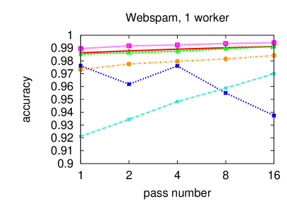
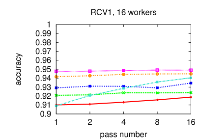
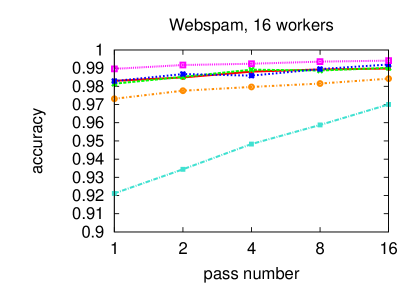
Here we experimentally compare the predictive performance of the local, the global, and the centralized update rules. We derived classification tasks from the two data sets described in Table 1, trained predictors using each training algorithm, and then measured performance on separate test sets. For each algorithm, we perform a separate search for the best learning rate schedule of the form with , . We report results with the best learning rate we found for each algorithm and task. For the minibatch case we report a minibatch size of but we also tried smaller sizes even though there is little evidence that they can be parallelized efficiently. Finally we report the performance of a centralized stochastic gradient descent (SGD) which corresponds to minibatch gradient descent with a batch size of 1.
| Name | # training data | # testing data |
|---|---|---|
| RCV1 | K | K |
| Webspam | K | K |
We omit results for the Delayed Global and Corrective update rules because they have serious issues with delayed feedback. Imagine trying to control a system (say, driving a car) that responds to actions after much delay. Every time an action is taken (such as steering in one direction) it is not clear how much it has affected the response of the system. If our strategy is to continue performing the same action until its effect is noticeable, it is likely that by the time we receive all the delayed feedback, we will have produced an effect much larger than the desired. To reduce the effect we can try to undo our action which of course can produce an effect much smaller than what was desirable. The system then oscillates around the desired state and never converges there. This is exactly what happens with the delayed global and corrective update rules. Delayed backpropagation is less susceptible to this problem because the update is based on both the global and the local gradient. Minibatch approaches completely sidestep this problem because the information they use is always a gradient at the current weight vector.
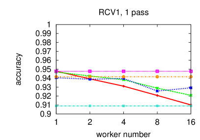
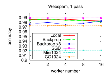
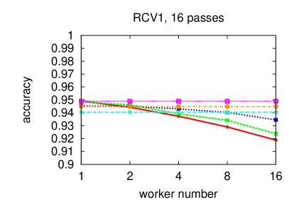
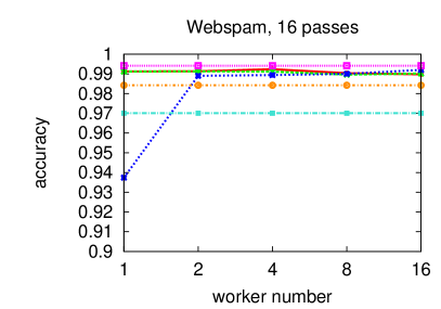
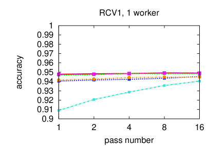
In Figure 6 we report our results on each data set. We plot the test accuracy of each algorithm under different settings. “Backprop x8” is the same as backprop where the gradient from the master is multiplied by 8 (we also tried 2, 4, and 16 and obtained qualitatively similar results)—we tried this variant as a heuristic way to balance the relative importance of the backprop update and that of the local update. In the first row of Figure 6, we show that the performance of both local and global learning rules degrades as the degree of parallelization (number of workers) increases. However, this effect is somewhat lessened with multiple passes through the training data and is milder for the delayed backprop variants, as shown in in the second row for the case of 16 passes. In the third and fourth rows, we show how performance improves with the number of passes through the training data, using 1 worker and 16 workers. Notice that SGD, Minibatch, and CG are not affected by the number of workers as they are global-only methods. Among these methods SGD dominates CG which in turn dominates minibatch. However, SGD is not parallelizable while minibatch CG is.
 |
 |
 |
 |
 |
 |
 |
 |
8 Conclusion
Our core approach to scaling up and parallelizing learning is to first take a very fast learning algorithm, and then speed it up even more. We found that a core difficulty with this is dealing with the problem of delay in online learning. In adversarial situations, delay can reduce convergence speed by the delay factor, with no improvement over the original serial learning algorithm.
We addressed these issues with parallel algorithms based on feature sharding. The first is simply a very fast multicore algorithm which manages to avoid any delay in weight updates by virtue of the low latency between cores. The second approach, designed for multinode settings, addresses the latency issue by trading some loss of representational power for local-only updates, with the big surprise that this second algorithm actually improved performance in some cases. The loss of representational power can be addressed by incorporating global updates either based on backpropagation on top of the local updates or using a minibatch conjugate gradient method; experimentally, we observed that the combination of local and global updates can improve performance significantly over the local-only updates.
The speedups we have found so far are relatively mild due to working with a relatively small number of cores, and a relatively small number of nodes. Given that we are starting with an extraordinarily fast baseline algorithm, these results are unsurprising. A possibility does exist that great speedups can be achieved on a large cluster of machines, but this requires further investigation.
References
- Amari, (1967) Amari, Shun-ichi. 1967. A theory of adaptive pattern classifiers. IEEE Transactions on Electronic Computers, 16, 299–307.
- Blum et al., (1999) Blum, A., Kalai, A., and Langford, J. 1999. Beating the hold-out: bounds for k-fold and progressive cross-validation. Pages 203–208 of: Proc. 12th Annu. Conf. on Comput. Learning Theory. ACM Press, New York, NY.
- Bottou, (2008) Bottou, Léon. 2008. Stochastic Gradient SVMs. http://leon.bottou.org/projects/sgd.
- Bryson and Ho, (1969) Bryson, Arthur Earl, and Ho, Yu-Chi. 1969. Applied optimal control: optimization, estimation, and control. Blairsdell Publishing Company.
- Chu et al., (2007) Chu, C., Kim, S. K., Lin, Y., Yu, Y., Bradski, G., Ng, A. Y., and Olukotun, K. 2007. Map-Reduce for Machine Learning on Multicore. In: Neural Information Processing Systems (NIPS) 19.
- Dekel et al., (2010) Dekel, Ofer, Gilad-Bachrach, Ran, Shamir, Ohad, and Xiao, Lin. 2010. Optimal Distributed Online Prediction using Mini-Batches. In: Learning on Cores, Clusters, and Clouds Workshop.
- Gilbert and Nocedal, (1992) Gilbert, J.C., and Nocedal, J. 1992. Global convergence properties of conjugate gradient methods for optimization. SIAM Journal on Optimization, 2(1), 21–42.
- Kivinen and Warmuth, (1995) Kivinen, J., and Warmuth, M. K. 1995. Additive versus exponentiated gradient updates for linear prediction. Pages 209–218 of: Proc. 27th Annual ACM Symposium on Theory of Computing. ACM Press, New York, NY.
- Langford et al., (2007) Langford, J., Li, L., and Strehl, A. 2007. Vowpal Wabbit Online Learning Project. http://hunch.net/?p=309.
- Langford et al., (2008) Langford, J., Strehl, A., and Wortman, J. 2008. Exploration Scavenging.
- Langford et al., (2009) Langford, J., Smola, A.J., and Zinkevich, M. 2009. Slow Learners are Fast. arXiv:0911.0491.
- Lewis et al., (2004) Lewis, David D., Yang, Yiming, Rose, Tony G., and Li, Fan. 2004. RCV1: A New Benchmark Collection for Text Categorization Research. The Journal of Machine Learning Research, 5, 361–397.
- Mann et al., (2009) Mann, G., McDonald, R., Mohri, M., Silberman, N., and Walker, D. 2009. Efficient Large-Scale Distributed Training of Conditional Maximum Entropy Models. In: Neural Information Processing Systems (NIPS).
- McDonald et al., (2010) McDonald, R., Hall, K., and Mann, G. 2010. Distributed Training Strategies for the Structured Perceptron. In: North American Association for Computational Linguistics (NAACL).
- Rahimi and Recht, (2008) Rahimi, A., and Recht, B. 2008. Random Features for Large-Scale Kernel Machines. In: Platt, J.C., Koller, D., Singer, Y., and Roweis, S. (eds), Advances in Neural Information Processing Systems 20. Cambridge, MA: MIT Press.
- Rosenblatt, (1958) Rosenblatt, F. 1958. The perceptron: A probabilistic model for information storage and organization in the brain. Psychological Review, 65(6), 386–408.
- Rumelhart et al., (1986) Rumelhart, D. E., Hinton, G. E., and Williams, R. J. 1986. Learning Internal Representations by Error Propagation. Chap. 8, pages 318–362 of: Parallel Distributed Processing. Cambridge, MA: MIT Press.
- Shalev-Shwartz et al., (2007) Shalev-Shwartz, Shai, Singer, Yoram, and Srebro, Nathan. 2007. Pegasos: Primal Estimated sub-GrAdient Solver for SVM. In: Proc. Intl. Conf. Machine Learning.
- Shi et al., (2009) Shi, Qinfeng, Petterson, James, Dror, Gideon, Langford, John, Smola, Alex, Strehl, Alex, and Vishwanathan, S. V. N. 2009. Hash Kernels. In: Welling, Max, and van Dyk, David (eds), Proc. Intl. Workshop on Artificial Intelligence and Statistics. Society for Artificial Intelligence and Statistics.
- Teo et al., (2009) Teo, Choon Hui, Vishwanthan, S. V. N., Smola, Alex J., and Le, Quoc V. 2009. Bundle Methods for Regularized Risk Minimization. J. Mach. Learn. Res. Submitted in February 2009.
- Weinberger et al., (2009) Weinberger, K., Dasgupta, A., Attenberg, J., Langford, J., and Smola, A.J. 2009. Feature Hashing for Large Scale Multitask Learning. In: Bottou, L., and Littman, M. (eds), International Conference on Machine Learning.