SPECTRAL POLARIZATION of the REDSHIFTED 21 cm ABSORPTION LINE TOWARD 3C 286

Abstract

A re-analysis of the Stokes-parameter spectra obtained of the $z$=0.692 21 cm absorption line toward 3C 286 shows that our original claimed detection of Zeeman splitting by a line-of-sight magnetic field, $B_{\rm los}$ = 87 $\mu$G is incorrect. Because of an insidious software error, what we reported as Stokes $V$ is actually Stokes $U$: the revised Stokes $V$ spectrum indicates a 3-$\sigma$ upper limit of $B_{\rm los}\ <$ 17 $\mu$G. The correct analysis reveals an absorption feature in fractional polarization that is offset in velocity from the Stokes $I$ spectrum by $-$1.9 km s^-1. The polarization position-angle spectrum shows a dip that is also significantly offset from the Stokes $I$ feature, but at a velocity that differs slightly from the absorption feature in fractional polarization. We model the absorption feature with 3 velocity components against the core-jet structure of 3C 286. Our $\chi^{2}$ minimization fitting results in components with differing (1) ratios of H I column density to spin temperature, (2) velocity centroids, and (3) velocity dispersions. The change in polarization position angle with frequency implies incomplete coverage of the background jet source by the absorber. It also implies a spatial variation of the polarization position angle across the jet source, which is observed at frequencies higher than the 839.4 MHz absorption frequency. The multi-component structure of the gas is best understood in terms of components with spatial scales of $\sim$ 100 pc comprised of hundreds of low-temperature ($T$ $\leq$ 200 K) clouds with linear dimensions of $<<$ 100 pc. We conclude that previous attempts to model the foreground gas with a single uniform cloud are incorrect.

1. INTRODUCTION

In order to detect magnetic fields in galaxies with significant redshifts, we began a search for Zeeman splitting of 21 cm absorption lines arising in damped lyman alpha systems (DLAs) toward background quasars (Wolfe et al. 2005) selected to be radio bright. The detection of Zeeman splitting yields the strength, direction, and redshift of the magnetic field, which is an advantage over measurements of Faraday rotation, which yield rotation measures accompanied with huge uncertainties in the strength and redshift of the $B$ fields along the sightlines to background quasars (Kronberg et al. 2008). In Wolfe et al. (2008) we reported the detection of Zeeman splitting in the $z$=0.692 DLA toward 3C 286. The purpose of this paper is to show that the reported detection was erroneous. In §2 we describe the errors that led to the claimed detection and describe our new data reduction procedures. In §3 we correct the previous errors and give a correct description of the polarization spectra. The new spectra are shown in §4.

In the absence of detectable Zeeman splitting we can only set an upper limit to the magnetic field in the $z$=0.692 DLA toward 3C 286. However, in this paper we discuss how the spatial distribution of the strong linear polarization of 3C 286 itself can be used in combination with observed spectral variation of linear polarization across the absorption profile of the redshifted 21 cm line to infer physical properties of the absorbing H I gas. We demonstrate how comparison between properties of the linearly polarized and unpolarized absorption spectra provides new information about the spatial structure of this gas on scales of $\sim$ 100 pc. We use the new data to determine both the kinetic temperature and hyperfine spin temperature of the gas, which in turn tells us about its thermal state. We use these results to evaluate the standard assumption of a large-scale, uniform cloud. We start by constructing models to describe the re-analyzed spectra in terms of multiple clouds distributed across the spatially extended structure of 3C 286. In §5.1 we use VLBI maps to exhibit the core-jet structure of 3C 286 near the 21 cm absorption frequency. In §5.2 we describe a two-cloud configuration to model the absorption feature. We use a chi square minimization technique to fit the model to the Stokes $I$ spectrum and the fractional polarization spectrum and show that the model does not work. In §5.3 we show how an adjustment in covering factors and the presence of velocity gradients in the cloud toward the polarized jet source results in a three-component model that provides an adequate fit to the Stokes $I$, fractional polarization, and polarization position-angle spectra. The implications of the results are discussed in §6. All the results are then summarized in §7.

Throughout this paper we use a WMAP cosmology in which ($h,{\Omega_{\rm m}},{\Omega_{\Lambda}}$) =(0.7, 0.3, 0.7).

2. OBSERVATIONS

We used the Green Bank Telescope in 2007 to observe the $z=0.692$ 21 cm absorption spectrum against 3C 286. We observed all four Stokes parameters simultaneously using the digital FX Spectral Processor, which provides all the necessary self- and cross-products; here “FX” means that first it Fourier transforms the input signal and then multiplies the voltage spectra with appropriate phase shifts. This technique is described in detail by Heiles et al. (2001) and Heiles (2001).

Our original paper reported a very statistically significant detection of circular polarization (Stokes $V$) for the 21-cm line DLA system against 3C 286. As Zeeman splitting, it translates to a line-of-sight field strength of 84 $\pm$9 $\mu$G. Subsequently, after re-observing 3C 286 in January and March 2009, we found that this detection is incorrect, basically because what we reported as Stokes $V$—circular polarization—is really Stokes $U$—linear polarization. The discussion below explains the origin of this error, which is a matter of a misplaced $90^{\circ}$ of phase.

2.1. Calibrating a Local Noise Source as a Secondary Calibrator Standard

The sky electric field is sampled by probes in the telescope feed. In our observations with the GBT, these two native polarizations are very close to being orthogonal linears. For convenience we denote the sampled voltage spectra (i.e., the Fourier transforms of the sampled voltages) as $X$ and $Y$. Apart from small corrections for nonorthogonality and other coupling, the Stokes parameters are obtained as follows:

$$I=XX+YY$$ (1a)

$$Q=XX-YY$$ (1b)

$$U=2{\cal R}(XY)$$ (1c)

$$V=2{\cal I}(XY)$$ (1d)

We tacitly assume that the voltage spectral products are time averages. Here $\cal R$ and $\cal I$ mean the Real and Imaginary parts, respectively. To clarify these equations and their discussion, we neglect the small corrections for nonorthogonality; these corrections are embodied in the feed’s Mueller matrix and are determined as discussed in §2.3.

In a heterodyne radio receiver the signal from the sky is amplified by mixing (multiplying) the sky signal by one or more locally-generated signals of known amplitude and phase. The resulting signal product, the gain $G_{e}$, is a complex number in which the amplitude is the real part and the phase the imaginary part. Between the receiver and the Spectral Processor there are a variety of electromagnetic components that alter the phase of the signal. Specifically, there are cables and optical fiber, each of which adds phase proportional to $2\pi L\over\lambda$, where $L$ is the length and $\lambda$ the wavelength of the signal in the particular cable. Thus the gain $G_{e}$ is a complex number. Moreover, some of these electromagnetic components have their own polarization properties that differ for $X$ and $Y$, and as a result we have $G_{e,X}$ and $G_{e,Y}$. For the complex portion of these gains, the only part of concern is the phase angle difference

$$\phi_{e}=\phi_{e,Y}-\phi_{e,X}$$ (2a)

where

$$\tan\phi_{e,Y}={{\cal I}(G_{e,Y})\over{\cal R}(G_{e,Y})}$$ (2b)

and a similar equation for $X$.

These complex gains must be calibrated and their effects removed. The standard technique is to inject perfectly correlated noise at the feed from a noise source, commonly called the “cal”. Like the sky signal, the correlated noise source injects voltages into the feed; unlike the sky signal, the cal’s noise is perfectly correlated and corresponds to 100% polarization. We compare the cal’s signal with that of a standard polarized calibration source of known flux to determine the equivalent antenna temperatures of the cal. We also compare the relative phase of the cal with that of the source, which relates the polarization of the cal to that of the sky.

In essence, we determine the gain of the cal in $X$ and $Y$ relative to the sky signal; these gains are complex and change with frequency. We assume the cal’s properties to remain constant with time. In subsequent observations, we use the cal’s deflection to determine the complex electronic gains $G_{e,X}$ and $G_{e,Y}$.

2.2. Using the Cal to Calibrate the Complex Gains

Consider the frequency dependence of equation 2a. The individual phase terms on the right-hand-side come from electronic components and from cables. The phase delays of most electronic components change relatively slowly with frequency. However, for cables, the phase delay is $2\pi L\over\lambda$ and the phase difference in equation 2a is $\Delta\phi={2\pi\Delta L\over\lambda}$, where $\Delta L$ is the length difference between $Y$ and $X$. In our experience, $\Delta\phi$ varies fairly rapidly with frequency. In particular, using the techniques described by Heiles (2001), for the current observations we find

$${d\Delta\phi\over d{\nu}}\approx{20\ \ {\rm deg\ MHz^{-1}}}$$ (3)

We have well-tested software that reliably performs this determination, and its correction (e.g. Heiles & Troland 2004). Unfortunately, however, this software had a bug, which we discovered on June 5, 2009 while we were analyzing both the 2007 and 2009 data. If we fed the software an array of spectra to correct, it performed correctly. But if we fed the software just a single spectrum, it didn’t apply any correction at all. Before the current observations, we had never used the software on individual spectra.

During our original 2007 observations this phase delay happened to average about 91 degrees at band center with a slope of about 20 deg/MHz; the phase delay fluctuated by at most a few degrees for all of our spectra. For our bandwidth of 625 kHz, the slope doesn’t matter much. Thus, the phase difference of $\sim 90$ degrees effectively interchanges the real and imaginary parts of the cross-correlation product. In turn, this changes the derived Stokes $V$ into Stokes $U$, and vice-versa. Fortunately, in our 2009 observations the phase delay was about 30 degrees, which alerted us to the error in the 2007 data. Although the precise cause of the change in phase delay between 2007 and 2009 is unknown, we note that a change in cable length in either polarization over the entire signal path between the feed and correlator could result in such a change.

2.3. The Mueller Matrix

We corrected for polarization impurities in the system by using the Mueller matrix formulation given by Heiles et al. (2001). The Mueller matrix relates the measured auto- and cross-correlation products to the actual Stokes parameters. With this procedure, one observes a linearly polarized calibrator over a range of parallactic angle $PA$ to derive seven parameters that describe the complex gains and coupling coefficients of the receiver system components. One then derives the Mueller matrix coefficients from algebraic combinations of these coefficients.

In the present paper, we observed 3C 286. This source is, for most purposes at cm wavelengths, the “gold standard” polarization calibrator. Specifically, the fractional polarization and polarization position angle of 3C 286 have been stable over four decades of observations across a wide range of frequencies above $\sim$ 1400 MHz (Tabara & Inouye 1980; B. Gaensler 2009 priv. comm.). While these properties have not been established at lower frequencies, the dominance of the large-scale jet at these frequencies argue against any time variations of these quantities at 840 MHz. Hence we had the fortunate circumstance of observing a source that also happens to be an excellent polarization standard. For about half of our observing days, we had enough $PA$ coverage to derive the Mueller matrix from our observed data for that particular day; thus, we could use our observed astronomical data to also determine the Mueller matrix elements—a form of “self calibration”. The derived corrections were closely the same from one day to another, although there were small differences. For any particular day’s observations, we used the matrix that was closest in time to that day; for about half the days, this matrix was obtained on that very day. This gives us great confidence in our polarization calibration.

Normally, one determines a single Mueller matrix for the observed band by averaging over the whole band. This leads to small calibration errors that change with frequency across the band, which in turn leads to small “baseline curvature” in the three polarization spectra. The latter are the fractional polarization $p(v)$, polarization position angle $\chi(v)$, and Stokes $V$ parameter $V(v)$; one normally fits a smooth baseline to these spectra and applies them as an ad-hoc correction.

Here, we took a different approach. 3C 286 is such a strongly polarized source that, for any one day, we could easily determine the seven receiver system parameters on a channel-by-channel basis. We then fit their frequency dependencies by performing a minimum-absolute-residual-sum (MARS) 3rd-degree polynomial fit. We used these fit coefficients to derive the Mueller matrix independently for each channel. With this, the polarization calibration is very accurate for each channel independently, so that any features in the polarized spectra are real, characterizing the sky instead of the system. In particular, it is neither appropriate nor necessary to subtract off an ad-hoc baseline in any of the polarized spectra. It is these accurately-calibrated spectra that we use and plot in this paper. Even with this self-calibration of each channel independently, there remain small residual inaccuracies, which result from applying Mueller matrices obtained on one day to data obtained on another day; this is probably responsible for the small spectral effects in the Stokes $V$ spectrum in Figure 1.

3. REANALYSIS

First, we fixed the above-mentioned software bug. Then we reanalyzed the data. We used the same software as before and determined the Mueller matrices in the usual way (see Heiles et al. 2001), as we did before. We applied the Mueller matrix corrections and the phase difference correction of equation 2a as we did before. We did three things differently:

1. We derived the linear polarization by fitting the Parallactic angle dependence of Stokes $U$. Stokes $U$ is a cross product and produces more reliable results, free of zero offsets, than Stokes $Q$, which is the difference between two large numbers. (As it happens, the results from Stokes $Q$ are indistinguishable from those of Stokes $U$).

2. We reduced the off-line (i.e., the 3C 286 continuum) spectral channels to ensure that we obtain the correct results. That is, we did not “subtract off the continuum baseline”. 3C 286 is the premier polarization calibrator in radio astronomy, and this ensures that our spectral line and continuum results correspond to what is known about 3C 286.

   The one wrinkle in this is that we have been unable to find a primary measurement of the polarization properties of 3C 286 at frequencies as low as ours, 840 MHz. While 3C 286 exhibits essentially zero change with frequency of polarization position angle above 1.4 GHz, we cannot be sure that the angle at 840 MHz isn’t somewhat different. We did not wish to address this question and therefore our reported polarization position angles have an arbitrary zero point.

3. We edited the data much more carefully than before, which produced only minor improvements.

4. THE PROPER DATA: STOKES PARAMETERS

Figure 1 shows a four-panel plot of the data (black curves), now reduced properly. No “baseline corrections” have been subtracted or applied. The data consists of 12.6 hrs of on-source integration obtained in 2007. The orange curves are least squares fits to the data. The top panel shows Stokes $I(v)/I$ (where $I$ is the off-line continuum intensity, which is independent of velocity $v$), which has an absorption line with a fractional absorption of about 5%. The frequency centroid determined by the fit to the Stokes I spectrum is 839.408348 $\pm$ 0.000046 MHz and its location is depicted by the vertical dot-dashed line. The corresponding redshift $z$=0.69215109$\pm$0.00000009. The second panel shows the percent polarization, $p(v)={\sqrt{(U(v)^{2}+Q(v)^{2})}}/I$, and the third panel shows the position angle $\chi(v)$ (zero point is arbitrary).

The linearly polarized $p(v)$ line also appears in absorption (i.e. the percent polarization goes down in the line) and its fractional polarized absorption is close to that for Stokes $I$. Its line center differs from the Stokes $I$ line center by $5.0\pm 0.25$ kHz. This $20\sigma$ difference has high statistical significance. Taken together, these two results are consistent with the absorbing gas covering both nonpolarized and polarized portions of the continuum source image, and the velocity of the part that covers the polarized portion differing from that covering the unpolarized portion by 5.0 kHz (which is about 1.8 km/s).

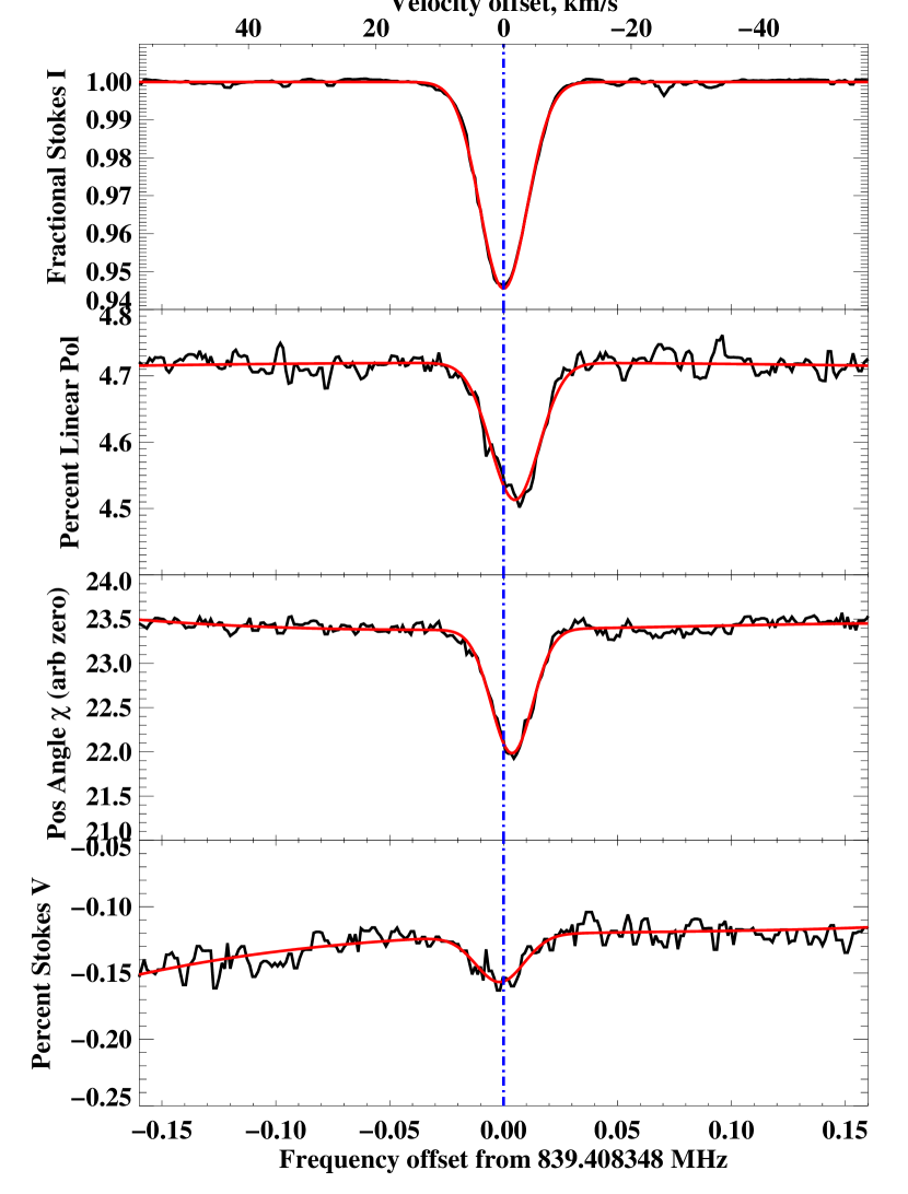
Figure 1.— Plots of Stokes parameters for 3C 286. From top to bottom, the panels are: the fractional absorption spectrum $I(v)/I$; fractional linear polarization $p(v)$; position angle of linear polarization $\chi(v)$; and fractional circular polarization $V(v)/I$. Fractional spectra are in percent and frequencies are barycentric in MHz offset from 839.408348 MHz. Black curves are data and orange curves are fits to the data.

The third panel shows that the line changes the position angle by about 1.5 degrees at line center, which is consistent with the absorbing gas covering only a fraction of the polarized source image and requires that the position angle of polarization of the continuum changes across the source image.

The fourth panel shows the percentage circular polarization $V(v)/I$. The absorption line exhibits a dip in fractional Stokes $V$ of $0.03\%$. However, we believe this apparent circular polarization is meaningless. The line is $5\%$ linearly polarized, and some of the total intensity and also the linear polarization will leak into Stokes $V$. The observed Stokes $V$ intensity of the line is only about $1\%$ of its linearly-polarized intensity. Errors in the Stokes parameters at these levels are not unexpected, because of the small day-to-day changes in the Mueller matrix elements.

5. CLOUD STRUCTURE PRODUCING THE ABSORPTION FEATURE

We now show that the GBT polarization spectra provide new and unique information about the kinematic and spatial structure of the gas that gives rise to 21 cm absorption toward 3C 286. In particular we note the following model-independent facts: (1) The difference between the velocity centroids of the Stokes $I$ and fractional polarization spectra is inconsistent with a single-cloud origin for the absorption. (2) The Gaussian shape of the absorption profile is plausibly explained through the cental limit theorem by the superposition of many small clouds. (3) The position-angle spectrum reinforces the conclusions drawn from the fractional polarization, but requires detailed modeling as described below. Besides studying the spatial and kinematic structure of the absorbing gas, we also investigate its two-phase structure; i.e., whether the gas is a cold neutral medium (CNM) with temperature $T$ $\sim$ 100 K, a warm neutral medium (WNM) with $T~{}\sim$ 8000 K (Wolfire et al. 1995), a thermally unstable phase with temperature between these two extremes, or some combination of any of these. Furthermore, we consider clues to the identity of the galaxy hosting the absorbing gas.

5.1. Core-jet structure of the radio source

The 21 cm absorption likely forms against a source with the core-jet configuration shown in Fig. 2 (Wilkinson et al. 1979). This VLBI map, obtained at 609 MHz, indicates that 3C 286 is an asymmetric source consisting of a compact core and an extended jet. The core, which covers a solid angle, $\Omega_{\rm core}{\approx}10{\times}5$ milli-arcsec² (mas²) with major-axis position angle equals 42^∘, contributes a flux density $S_{\nu}(609)$=3.5 Jy, while in the case of the jet $\Omega_{\rm jet}$ =40$\times$15 mas², P.A.=42^∘, and $S_{\nu}(609)$=14 Jy. Since a similar core-jet structure is detected at 329 MHz, 1667 MHz (Simon et al. 1980), 5 GHz (Jiang et al. 1996; Cotton et al. 1997), and 15 GHz (Kellermann et al. 1997, priv. comm.), it is safe to assume that such a structure is present at the absorption frequency of 839.4 MHz. Adopting the spectral indices measured by Simon et al. (1980) of ${\alpha_{\rm core}}=-0.29{\pm}$0.15 and $\alpha_{\rm jet}=-0.55$, we find that $S_{\nu}^{\rm core}$${\approx}$3.2 Jy and $S_{\nu}^{\rm jet}$$\approx$11.7 Jy at $\nu$ $\approx$ 840 MHz.

While the polarization structure of 3C 286 has not been detected at low frequencies, VLBI measurements of all four Stokes parameters have been obtained at 5 GHz (Jiang et al. 1996; Cotton et al. 1997; Cotton 2010 [priv. comm.]). These data show that unlike most quasar VLBI sources, the fractional polarizations, i.e., fraction of total surface brightness in $\sqrt{U^{2}+Q^{2}}$, where $U$ and $Q$ are the Stokes parameters, of the core and jet are comparable. More specifically, the ratio of jet to core polarized surface brightnesses is about 0.4.

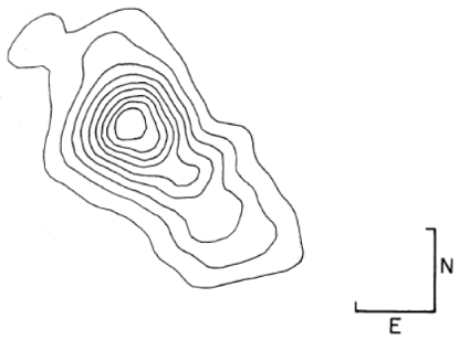
Figure 2.— VLBI map of 3C 286 at 609 MHz (Wilkinson et al. 1979). Continuum structure exhibits an unresolved core source to the north east and an extended jet source to the south west. Orthogonal straight lines are 0.02 arcsec in length corresponding to 142 pc at the absorber.

Nevertheless the ratio of polarized flux densities $P^{jet}/P^{core}$ $\approx$ 5 owing to the much larger solid angle subtended by the jet, where the polarized flux density $P=\sqrt{U^{2}+Q^{2}}$. Because of the steeper spectral index of the jet, it is reasonable to assume that this ratio increases with decreasing frequency. As a result, we shall ignore the core source when computing absorption in Stokes $U$ and $Q$ parameters, or equivalently in the spectrum of polarized flux density $P$ (note, $P=pI$) and polarization position angle $\chi=0.5{\times}$arctan($U/Q$). We check the self-consistency of this assumption in $\S$ 7.

5.2. Two Cloud Model

We now describe the procedures used to model the Stokes parameter spectra.

5.2.1 Model Description

Figure 3.— Foreground clouds (grey) superposed on VLBI map from Fig. 2. Cloud 2 at NE completely covers core source, while cloud 1 toward SW partially covers resolved jet source. Cloud 1 is shaded darker to illustrate its larger 21 cm optical depth. Light blue shading indicates that region emitting polarized radiation is the jet. Thick red bars depict direction of E vector polarization. Orthogonal straight lines are 0.02 arcsec in length corresponding to 142 pc at the absorber.

To account for the absorption spectrum we first adopt a simplified model, illustrated in Fig. 3, comprised of one uniform H I ‘cloud’ toward the jet (cloud 1) and another uniform H I ‘cloud’ toward the core (cloud 2). A single cloud model is ruled out by past VLBI observations of the 839.4 MHz absorption feature that indicated an inhomogeneous structure of the absorbing gas. The velocity difference between the maximum depths of the phase-shift and fringe amplitude spectra detected by a two-element VLBI experiment (Wolfe et al. 1976) indicates a velocity difference between the H I towards the core and jet sources. As a result the relative change in Stokes $I$ parameter at velocity $v$ is given by

$${\Delta}{I(v)/I}=\sum_{i=1}^{n_{c}}C_{i}f_{i}{\Biggl{[}}{\rm exp}{\biggl{(}}-{\tau_{i}(v){\biggr{)}}}-1{\Biggr{]}}$$ (4)

where the number of clouds $n_{c}$=2, $C_{1}$ and $C_{2}$ are the area covering factors of the gas toward the jet and core, $f_{1}$ and $f_{2}$ are the fractions of Stokes $I$ flux density in the jet and the core sources, and ${\tau_{1}(v)}$ and ${\tau_{2}(v)}$ are the 21 cm optical depths averaged across the areas subtended by jet and core at the absorber. Note, $I$ in the denominator of eq. (4) is the continuum Stokes $I$ parameter extrapolated across the 21 cm absorption line.

In order to fit the model to the data we made the following assumptions (see Fig. 3): First, because most of the polarized flux density arises from the jet, we assume the absorption spectrum of polarized flux density, $P({v})$, arises only in ‘cloud’ 1. Since the line center of the $P({v})$ spectrum is shifted by $+$ 5.0$\pm$0.25 kHz ($-$1.8$\pm$0.1 km s^-1) relative to the line center of the Stokes $I({v})$ spectrum, we assume that the velocity centroid of cloud 1 is lower than that of cloud 2. Second, the shift in polarization position angle with frequency , $\Delta\chi({v})$$\equiv$${\chi}({v})$ $-$ $\chi_{\rm cont}$ (where $\chi_{\rm cont}$ is the polarization position angle averaged over the continuum source), indicates that ‘cloud’ 1 partially covers source 1, i.e., $C_{1}$ $<$ 1, and the intrinsic value of $\chi$ varies across the source, as is observed in VLBI experiments at high frequencies (Jiang et al. 1996; Cotton et al. 1997). With a covering factor $C_{1}$ $<$ 1, the position angle of polarized flux behind the cloud is weighted less in the line than in the continuum, thereby causing a shift of position angle in the line. Third, because of the smaller dimensions of the core source, we assume $C_{2}$=1. Fourth, we assume Gaussian velocity distributions for each cloud, in which case the optical depth of the $i^{\rm th}$ cloud at velocity $v$ is given by

$$\tau_{i}(v)={\tau_{0,i}}{\times}{\rm exp}{\Biggl{[}}-{\biggl{(}}(v-v_{i})/{\sqrt{2}}{\sigma_{v,i}}{\biggr{)}}^{2}{\Biggr{]}}$$ (5)

where $v_{i}$ and and $\sigma_{v,i}$ are the velocity centroid and velocity dispersion of the $i^{th}$ cloud. In the case of 21 cm absorption the central optical depth

$${\tau}_{0,i}={{{N}_{\rm HI,i}}/{\biggl{(}}{4.57{\times}10^{18}{\sigma}_{v,i}}{T_{s,i}}}{\biggr{)}}$$ (6)

where $T_{s,i}$ is the spin temperature and $\sigma_{v,i}$ is in units of km s^-1. Fifth, because the polarized radiation is assumed to be emitted only by the jet source, the relative change in fractional polarization is given by

$${\Delta P(v)}/P=C_{1}{\Biggl{[}}{\rm exp}{\biggl{(}}-{\tau_{1}}(v){\biggr{)}}-1{\Biggr{]}}.$$ (7)

where we again extrapolate across the line to obtain $P$ in the denominator of the last equation. The geometry of the model is illustrated in Fig. 3

5.2.2 Model Fits To The Data

We adopted an incremental approach by first modeling the $\Delta I/I$ spectrum alone. When a successful fit was found we then fitted $\Delta I/I$ together with either the $\Delta P/P$ or $\Delta\chi$ spectrum simultaneously. If a successful fit were obtained, we followed up by fitting $\Delta I/I$, $\Delta P/P$, and $\Delta\chi$ spectra simultaneously. The 1-$\sigma$ errors, which were derived by computing the standard deviations from portions of the spectra displaced from the absorption features, are as follows: $\sigma_{\Delta I/I}$=0.00050, $\sigma_{{\Delta P}/P}$=0.0034, and $\sigma_{\Delta\chi}$=0.042^∘.

We obtained the relevant parameters by fitting the model to the data with the Levenberg-Marquardt method that makes use of the non-linear chi square minimization routine, $mrqmin$ (Press et al. 1996). For the ${\Delta I}/I$ spectrum we fixed the area covering fractions $C_{1}$=0.5 and $C_{2}$=1.0 as discussed above, but allowed the other parameters to float after making initial guesses that were guided by the discussion in $\S$ 5.2.1. Specifically we solved for $N_{\rm HI,i}/T_{s,i}$ , $v_{i}$, $\sigma_{\rm v,i}$, and $f_{i}$. A successful fit was found and the output parameters were then used as inputs for fitting the $\Delta I/I$ and $\Delta P/P$ spectra simultaneously. The results are shown in Fig. 4.

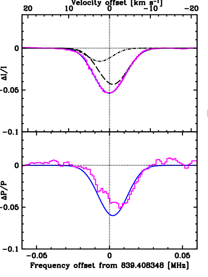
Figure 4.— Stokes spectra of 3C 286. Solid curves are two-cloud fits and data given by histograms. Top panel shows $\Delta I/I$ spectrum. Spectrum with dashed curve showing solution for cloud 1 and dot-dashed curve for cloud 2. Bottom panel shows $\Delta P/P$.

While the fit to the $\Delta I/I$ spectrum appears to be quite accurate, the fit including the $\Delta P/P$ spectrum has a chi square per degree of freedom, $\chi^{2}/{\nu}$=12.6, which is unacceptable. The reasons for the failure of the model are straightforward. Both the depth of the model $\Delta P/P$ absorption feature and the location of its frequency centroid are in significant disagreement with the data. Altering the input parameters to get a better fit to the $\Delta P/P$ spectrum does not solve the problem, because such changes also alter the $\Delta I/I$ spectrum, which result in significant disagreement between the model and observed $\Delta I/I$ spectra. The dilemma is that while cloud 1 produces both the $\Delta P/P$ spectrum and most of the $\Delta I/I$ spectrum, the difference between the velocity centroids of these spectra are too large to be modeled with a single velocity component. Because of a similar difference between the frequency centroids of the $\Delta\chi$ and $\Delta I/I$ spectra, it is clear that the polarized radiation is incident on a third velocity component. As a result we abandon the two-cloud model in favor of a three-component model to which we now turn.

5.3. Three Component Model

.

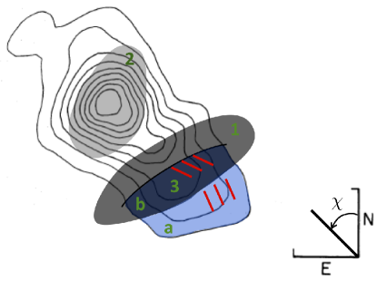
Figure 5.— Same as Fig. 3 except that cloud 1 covers both unpolarized (white) and polarized (blue) portions of the jet. Gas in cloud 1 toward polarized portion is called component 3, which has a velocity centroid lower than that of the entire cloud 1. Note that intrinsic polarization position angle $\chi$ (where $\chi$ is defined to increase positively in counter-clockwise direction from due North) decreases along the source in the SW direction. $\chi=\chi_{b}$ for the area of the polarized jet behind cloud 1 (i.e., behind component 3) and $\chi=\chi_{a}$ for the area of the jet not behind cloud 1. Orthogonal straight lines are 0.02 arcsec in length corresponding to 142 pc at the absorber.

For this model we again ignore polarized radiation from the core and assume that it is emitted only by the jet. Again we assume that most of the flux from the jet is in Stokes $I$. But we now assume that part of the jet has low or vanishing polarization and that ‘cloud’ 1 covers both this unpolarized portion of the jet and that part of the jet which emits polarized radiation (the faint blue section of the source in Fig. 5): the covering factor for the latter is $C_{3}$. We further assume the presence of a velocity gradient in ‘cloud’ 1 such that the velocity centroid for the Stokes $I$ spectrum is again $v_{1}$, but for the $\Delta P/P$ spectrum is now $v_{3}$ (see Fig. 5). As a result we now have

$${\Delta P(v)}/P=C_{3}{\Biggl{[}}{\rm exp}{\biggl{(}}-{\tau_{3}}(v){\biggr{)}}-1{\Biggr{]}}.$$ (8)

where $\tau_{3}(v)$ is the 21 cm optical depth of the gas in cloud 1 toward the polarized portion of the jet source: the velocity centroid of this gas is $v_{3}$. Therefore, this model has velocity components centered on $v_{1},v_{2},{\rm and}\ v_{3}$.

Since we shall also consider fits to the $\Delta\chi$ spectrum in this case, we develop a model for the intrinsic change in polarization position angle across the jet source. We assume that $\chi=\chi_{a}$ for the polarized flux density emitted by the fraction of the jet source that is not incident on the cloud and $\chi=\chi_{b}$ for the fraction of emitted polarized flux density that is incident on the cloud. Noting that the net flux densities in Stokes $Q$ and $U$ parameters are given by $Q=Q_{a}+Q_{b}$ and $U=U_{a}+U_{b}$, and $\chi$=0.5$\times$arctan($U/Q$), we find that

$${\chi}(v)={1\over 2}{\rm arctan}{\Biggl{[}}{r{C_{3}{\rm tan}(2{\chi_{b}}){\rm exp}(-\tau_{3}(v))+(1-C_{3}){\rm tan}(2{\chi_{a}})}\over{rC_{3}{\rm exp}(-\tau_{3}(v))+1-C_{3}}}{\Biggr{]}.}$$ (9)

Here $r$=$<{\cal I}_{Q}>_{b}$/$<{\cal I}_{Q}>_{a}$, where $<{\cal I}_{Q}>_{a}$ and $<{\cal I}_{Q}>_{b}$ are the surface brightnesses in Stokes $Q$ averaged over regions a and b respectively, and we make use of the relation $Q_{b}/Q_{a}=rC_{3}/(1-C_{3})$. The observed value of $\chi$ averaged over the unattenuated continuum source, $\chi_{\rm cont}$, is obtained from the last equation by setting $\tau_{3}$=0. The difference between $\chi$ in the line and $\chi_{\rm cont}$ is denoted by $\Delta\chi(v)$$\equiv$$\chi-\chi_{\rm cont}$.

We fitted the three-component model parameters to the spectra as follows. First, observing that the parameters characterizing the Stokes $\Delta I/I$ spectrum are independent of those characterizing the $\Delta P/P$ and $\Delta\chi$ spectra, we did not fit the three Stokes spectra simultaneously. Rather, we fitted the $\Delta I/I$ spectrum alone, and then the $\Delta P/P$ and $\Delta\chi$ spectra simultaneously. Given the reasonable fit to the $\Delta I/I$ spectrum discussed in $\S$ 5.2, we adopt the parameters found for clouds 1 and 2 in that fit here. Second, in the case of the polarized spectra we need to find the gas parameters, $N_{{\rm HI},3}/T_{s,3}$, $v_{3}$, $\sigma_{v,3}$, and $C_{3}$ as well as the source parameters $r$, $\chi_{a}$, and $\chi_{b}$. For the source parameters, we are guided by single-dish polarization measurements above 1.5 GHz that show the continuum polarization position angle for the entire source $\chi_{\rm cont}$=33$\pm$5^o (Tabara and Inoue 1980). The VLBI polarization data at 5 GHZ (Jiang et al. 1996; Cotton et al. 1997; Cotton 2010 priv. comm.) further show that along the jet $\chi$ decreases with increasing distance from the core source (i.e., in the SW direction) by as much as $\approx$ 40^∘ which is consistent with the orientation of the polarization bars in Fig 5. We found that the $\Delta\chi(v)$ line spectral feature is more naturally explained by a large central optical depth $\tau_{0,3}$ combined with a low covering factor $C_{3}$ rather than vice versa. By contrast, $C_{3}$ and $\tau_{0,3}$ are degenerate in the case of the $\Delta P/P$ spectrum (see eq. (8)).

	Gas Properties					Source Properties
Cloud	${\tau_{0,i}}$	$N_{\rm HI}$,i/$T_{s,i}$	$v_{i}$a	$\sigma_{v,i}$		$C_{i}$	$f_{i}$	$\chi_{a}$	$\chi_{b}$
		cm-2K-1	km s-1	km s-1				deg.	deg.
1	0.128$\pm$0.005	(2.03$\pm$0.01)${\times}10^{18}$	$-$0.82$\pm$0.02	3.48$\pm$0.02		0.5	0.72	….	….
2	0.057$\pm$0.005	(7.94$\pm$0.10)${\times}10^{17}$	$+$2.37$\pm$0.07	3.05$\pm$0.07		1.0	0.28	….	….
3	0.280$\pm$0.004	(4.40$\pm$0.02)${\times}10^{18}$	$-$1.44$\pm$0.04	3.42$\pm$0.04		0.2b	$>$0.40c	2.70$\pm$0.9	43.6$\pm$0.9

Table 1Properties of Clouds and Source Causing the Absorption Feature

(a) Velocity $v$=0 corresponds to $z$=0.69215109, shown as dotted vertical lines in Figs.1,4, and 6.
(b) Fraction of polarized flux density incident on “cloud 3”.
(c) Fractional area of jet source emitting polarized radiation, assuming $r$=1.

We used $mrqmin$ to determine the cloud 1 and cloud 2 parameters by fits to the $\Delta I/I$ spectrum. As discussed above, the parameters of the third velocity component were found by separately fitting the $\Delta P/P$ and $\Delta\chi$ spectra together. This is possible since the polarized spectra are independent of the cloud 1 and 2 parameters, while the Stokes $\Delta I/I$ spectrum is independent of the component 3 parameters. After trials with several values of $C_{3}$ we fixed $C_{3}$=0.2 at the outset. Larger values of $C_{3}$ must be accompanied by smaller values in $\tau_{0,3}$ in order to maintain the observed value of $\Delta P/P$ (see eq. 8), but an increase in $C_{3}$ generates unacceptably large values of $\chi_{b}-\chi_{a}$ in order to retain the maximum dip of $\Delta\chi$$\approx$ $-$1.5^∘(see eq. 9). On the other hand smaller values of $C_{3}$ imply larger values of the ratio $<{\cal I}_{Q}>_{b}/<{\cal I}_{Q}>_{a}$, i.e. larger variations of polarized surface brightness across the source, than observed at 5 GHz (Jiang et al. 1996; Cotton et al. 1997). We considered letting $C_{3}$ be one of the floating variables, but decided to let it remain fixed, because the spatial variation of $\chi$ across the jet is at best a qualitative rather than a robust constraint. For these reasons we fixed $r$=1 at the outset (where $r$ is the ratio of average Stokes $Q$ surface brightnesses in region b relative to a), but let the remaining parameters float.

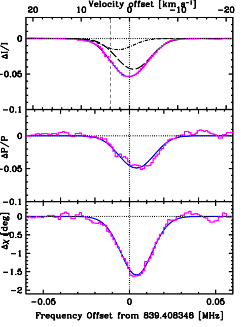
Figure 6.— Stokes spectra of 3C 286. Solid blue curves are three-component fits and data are magenta histograms. Top panel shows $\Delta I/I$ spectrum with cloud 1 and 2 solutions as dashed and dot-dashed black curves. Middle and bottom panels show $\Delta P/P$ and $\Delta\chi$ spectra. Model parameters are in Table 1. Vertical dotted line at offsets =0 corresponds to centroid of Stokes $I$ feature at $z$=0.69215109$\pm$0.0000000109. Dashed vertical line in top panel at $v$=4.21$\pm$0.11 km s^-1 shows velocity predicted by the optical redshift at $z$=0.69217485$\pm$0.00000058 (Wolfe et al. 2008).

The results are shown in Fig. 6, which plots model and observed spectra. The output parameters are listed in Table 1 along with 1-$\sigma$ errors. These were obtained from $\Delta{\chi}^{2}$ confidence ellipses containing 68$\%$ of the distributed data by projecting the ellipses onto each parameter axis (see Press et al. 1996). We did this for all possible pairs of the parameters in Table 1 and chose the largest value of the projection as the 1-$\sigma$ error. While the fit to the $\Delta I/I$ spectrum appears to be quite good, the chisquare per degree of freedom $\chi^{2}/{\nu}$=1.73, which corresponds to a probability of $\approx$10^-8 that ${\chi}^{2}$ exceeds 294 for 169 degrees of freedom. One reason for the elevated ${\chi}^{2}/{\nu}$ is that our model is undoubtedly inadequate given the $\approx$ 100:1 signal-to-noise ratio of the $\Delta I/I$ data. In principle we could improve the fit by adding more velocity components. But this would be an unconstrained ad hoc procedure, given our limited knowledge of the source-gas configuration, and thus we decided against it. The main reason for the high value of ${\chi}^{2}/{\nu}$ is that the largest contribution to ${\chi}^{2}$ comes from the relatively large scatter of the data around the model between 839.385 MHz and 839.397 MHz (i.e., between $\Delta\nu$=$-$ 0.023 and $-$ 0.011 MHz in Fig. 6). As the cause of this effect is currently uncertain, we attribute it to some unknown systematic error.

The fits to the polarized spectra result in $\chi^{2}/{\nu}$=1.54. This corresponds to a probability of $\approx$ 3$\times$10^-10 that ${\chi}^{2}$ exceeds 536 for 348 degrees of freedom. The reasons for the high value of ${\chi}^{2}/{\nu}$ in this case stems from the small, $\approx$ 3 kHz, difference between the velocity centroids of the $\Delta P/P$ and $\Delta\chi$ spectra. In contrast to the velocity difference between the centroids of the polarized and Stokes $I$ spectra, this effect is difficult to understand. In any plausible model the velocity centroids of the $\Delta P/P$ and $\Delta\chi$ spectra coincide with the centroid of the optical-depth velocity distribution (see eqs. 4, 8 and 9). We tested the possibility that the error might be due to a constant frequency offset between the $\Delta P/P$ and $\Delta\chi$ profiles by shifting the frequency scale of the $\Delta P/P$ spectrum. We found that $\chi^{2}/{\nu}$ decreased to a minimum of 1.48 when the shift was one frequency pixel (i.e., 1.2 kHz). However, the improvement of the fit was insufficient for the error to be a frequency offset. More likely this is also an unknown systematic error. Adding another velocity component doesn’t help since though it might improve the fit to the $\Delta P/P$ spectrum at 839.405 MHz, it also worsens the fit to the $\Delta I/I$ spectrum. Despite these problems, the model provides an adequate fit to the data, given that our goal is to determine a general picture of the cloud structure rather than obtain a precise evaluation of cloud sizes, locations, etc. As a result we shall adopt the three-component model in further discussions.

6. DISCUSSION

In this section we discuss implications of the models used to describe the 21 cm absorption in 3C 286.

6.1. Cloud and Galaxy Properties

In $\S$ 5.3 we discussed the three-component model used to model the $\Delta I/I$, $\Delta P/P$, and $\Delta\chi$ absorption spectra. As illustrated in Fig. 5 the three-component model is actually based on two clouds. One cloud (cloud 2) completely covers the core source. The other cloud (cloud 1) partially covers the jet source, and contains a velocity gradient such that the part of the cloud toward the polarized portion of the jet (component 3) causes the velocity centroid of the polarized spectra to be offset in velocity from the unpolarized $\Delta I/I$ spectrum. We simplified the model by letting component 3 be a uniform sub-region of cloud 1 with a velocity centroid, velocity dispersion, and 21 cm optical depth that differ from their values in the parent cloud. Table 1 indicates that the polarization position angle for the part of the source absorbed by the foreground cloud is $\chi_{b}$=43.6^∘. Because the ratio of the Stokes parameters, $U/Q$=tan(2$\chi$), the predicted ratio $U/Q$=20.4. By contrast, $U/Q$=0.046 toward the part of the jet that bypasses the absorbing gas where the model predicts $\chi_{a}$=2.67^∘. This is consistent with the independent Stokes $U$ and $Q$ absorption spectra, which show a clear detection of the absorption feature in Stokes $U$ but not in Stokes $Q$. The absorption feature, which is detected at a signal-to-noise ratio of about 20:1 in Stokes $U$, is predicted to be below the 1-$\sigma$ noise level in Stokes $Q$. The model also predicts $\chi_{cont}$=38^∘ for the position angle integrated over the entire source, which is consistent with single-dish measurements of 33$\pm$5^∘ at 1.5 GHz (Tabara & Inoue 1980). Our model predicts that the intrinsic polarization position angle of the jet decreases by $\chi_{a}-\chi_{b}$= $-$40.9^o in the SW direction (see Fig. 5). Polarization maps at 5 GHZ (Jiang et al. 1996; Cotton et al. 1997) do show shifts by about this amount in the sense of decreasing $\chi$ along the jet axis in the SW direction. However, the value of $\chi$ at the extreme edge of the jet appears to be greater than our prediction of $\chi_{a}$=2.67^∘. These predictions could be checked with VLBI polarization measurements at lower standard frequencies such as 609 MHz.

Next we turn to the properties of the absorbing gas. The large projected areas subtended by the sources at the absorber ($A_{\rm core}$$\approx$70${\times}$35 pc² for the core and $A_{\rm jet}$$\approx$280${\times}$60 pc² for the jet) likely indicate that the gas causing 21 cm absorption in 3C 286 is comprised of many interstellar clouds. In the Galaxy a beam with area $A_{\rm jet}$ directed perpendicular to the plane of the disk would subtend $\cal N_{\rm CNM}$$\approx$1000 CNM (i.e., cold neutral-medium [Wolfire et al. 1995]) clouds. This is because $\cal N_{\rm CNM}$=$n_{CNM}$${\times}A_{\rm jet}$$\times$2$H$ where the space density of CNM clouds $n_{CNM}$ $\approx$ 3$\times$10^-4 pc^-3 (McKee & Ostriker 1977) and the disk half-thickness $H$ $\approx$ 100 pc. This value of $\cal N_{\rm CNM}$ is a lower limit, since $\cal N_{\rm CNM}$=$n_{CNM}$$\times$$A{\times}$2$H$/cos($i$) for a disk with inclination angle $i$. For the core source $\cal N_{\rm CNM}$$\geq$60. As a result the Gaussian shape of the absorption profile is naturally explained as the optical-depth weighted sum of multiple Gaussians (i.e., the central limit theorem).

Note that the central velocities of the Gaussians are likely superposed on large-scale velocity gradients present both in ‘cloud’ 1 toward the jet and ‘cloud’ 2 toward the core. While such a gradient in ‘cloud’ 1 is required to explain the velocity shifts between the stokes $I$ and polarized spectra, as explained above, the necessity for a gradient in ‘cloud’ 2 stems from the approximate agreement between the optical redshift and redshift of ‘cloud’ 2 illustrated in Fig. 6. This implies that the optical continuum source is, as expected, physically associated with the compact radio core. The small, but significant, difference between these redshifts further suggests that since the optical beam size is small compared to the dimensions of ‘cloud’ 2, the optical beam samples only a limited portion of the velocities spanned by the gradient in ‘cloud’ 2. Therefore, although the UV resonance lines form in gas within ‘cloud’ 2, the velocity centroids formed by averaging over the optical and wider radio beams need not be equal.

To determine whether the absorbing gas is CNM, WNM, or something else we need to determine its kinetic temperature, $T_{k}$. Assuming the foreground gas covers the entire source with a uniform cloud characterized by $\sigma_{v}$ = 3.75 km s^-1 (Wolfe et al. 2008), one finds an upper limit of $T_{k}^{\rm max}$=1690 K. If we further assume that $N_{\rm HI}$ equals the UV-determined value of 1.77$\times$10²¹ cm^-2(e.g. Wolfe & Davis 1978; Kanekar 2003a), then eq. (6) implies $T_{s}$=1035 K, since the central 21 cm optical depth $\tau_{0}$=0.10 (Wolfe et al. 2008). Because $T_{s}\ <T_{k}\ <T_{k}^{\rm max}$ for diffuse warm gas (Liszt 2001), these results would indicate the gas is neither standard CNM where $T_{k}{\approx}$ 80 K nor standard WNM where $T_{k}$ $\approx$ 8000 K (Wolfire et al. 1995), but rather resembles the thermally unstable phase found by Heiles & Troland (2003) in the Galaxy ISM.

On the other hand the frequency-dependent change in polarization position angle across the absorption feature (panel 3 in Fig. 5) provides strong evidence against the assumption of a single uniform cloud (see $\S$ 5.4). From the values of $\sigma_{v,i}$ in Table 1 we find that $T_{k,i}^{\rm max}$=1450 K, 1115 K, and 1400 K for gas in velocity components 1, 2, and 3. If we again assume that $N_{\rm HI}$_,i=1.77$\times$10²¹ cm^-2 in each case, the values of $N_{\rm HI}$_,i/$T_{s,i}$ in Table 1 indicate that $T_{s,1}$=892 K $T_{s,2}$=2230 K, and $T_{s,3}$=394 K. However, since the values of $N_{\rm HI}$_,i/$T_{s,i}$ in Table 1 are spatial averages over dimension much larger than the $\approx$ 1 lt. yr. size of the UV continuum, it is unlikely that the UV determined value of $N_{\rm HI}$ applies to the gas in each component, nor that each component has the same value of $N_{\rm HI}$. It is equally plausible to assume that $N_{\rm HI}$ averaged across cloud 1 is a factor of 2 lower than the UV determined value, and $C_{1}$ equals 0.25 rather than 0.5. In that case $T_{s,1}$=223 K. Similarly if $N_{\rm HI}$_,3=$N_{\rm HI}$_,1, then $T_{s,3}$=197 K. Since these are physically plausible temperatures for CNM gas with the low metal abundances inferred for this absorber (Wolfe et al. 2008), it is reasonable to assume they represent kinetic temperatures. Interestingly, the assumption $N_{\rm HI}$_,2=1.77$\times$10²¹ cm^-2 results in the unreasonable prediction that $T_{s,2}$ is higher than $T_{k,2}^{\rm max}$: we take this as direct evidence that $N_{\rm HI}$_,2 is lower than 1.77$\times$10²¹ cm^-2 and/or $C_{2}$ $<$ 1, thereby implying that cloud 2 could also be CNM. Of course, we cannot entirely rule out the possibility that the gas is in a thermally unstable phase. But the above arguments in addition to the results from the VLBI line experiment, which indicates individual components toward the core and jet with kinetic temperatures $T_{k}$ $<$ 500 K (Wolfe et al. 1976), make a compelling case that the gas causing 21 cm absorption in 3C 286 is mainly CNM. Although this conclusion is at odds with the anti-correlation between $T_{s}$ and [M/H] found by Kanekar et al. (2009b), the evidence provided by our polarization measurements suggests either that physical conditions in this absorber deviate from typical conditions in DLAs or that most values of $T_{s}$ deduced from UV-determined values of $N_{\rm HI}$ are poor indicators of $T_{k}$.

Identification of the galaxy hosting the absorbing gas is difficult to ascertain. Le Brun et al. (1997) used HST images to tentatively identify an object (2c in their nomenclature) as the leading candidate for the host. Although its absolute magnitude $M_{B}=-20.1$ (in our cosmology) suggests a massive galaxy, the metallicity [M/H]=$-$1.6 of the absorbing gas (Wolfe et al. 2008) is at the low end for this redshift, which suggests a low-mass galaxy (Tremonti et al. 2004). Although the area subtended by 3C 286 at the absorber would encompass over 1000 CNM clouds, the 3.75 km s^-1 velocity dispersion of the absorption feature more closely resembles that of a single cloud rather than an ensemble of clouds. But this might be explained by a reduced supernovae input of mechanical energy into gas comprised of many clouds. This is consistent with the low metallicity and absence of C II^∗ absorption both of which indicate a lower than normal SFR (Wolfe et al. 2008). As a result, the evidence accumulated so far suggests that the gas causing 21 cm absorption in 3C 286 is embedded in a massive galaxy with a low SFR.

6.2. Limits on Variations of Physical Constants

The difference between the optical redshift, $z_{\rm opt}$, and radio redshift, $z_{\rm radio}$, places limits on variations of physical constants between the absorption epoch and the present, which is given by

$${\Delta}{\ln}({\alpha}^{2}g_{p}{m/M})=|(z_{\rm opt}-z_{\rm radio})/(1+z_{\rm radio})|,$$ (10)

Here $\alpha$ is the fine structure constant, $g_{p}$ is the gyromagnetic ration of the proton, and $m/M$ is the electron-to-proton mass ratio (Wolfe et al. 1976). Because the radio redshift $z_{\rm radio}$=0.69215109$\pm$0.0000000109 and the optical redshift $z_{\rm opt}$=0.69217485$\pm$0.00000058, ${\Delta}{\ln}({\alpha}^{2}g_{p}{m/M})$=4.2 km s^-1 $\pm$ 0.10 km s^-1 (in velocity units) where the error is dominated by the uncertainty in $z_{\rm opt}$. However, this estimate ignores the much larger systematic error determined from night-to-night changes in wavelength calibration on HIRES, which can be as large as 2 km s^-1 (Kanekar et al. 2010). Therefore, adopting the 4.2 km s^-1 difference as a conservative 2$\sigma$ upper limit, we find ${\Delta}{\ln}({\alpha}^{2}g_{p}{m/M})$ $<$ 1.4$\times$10^-5 in the redshift interval $z$=[0, 0.692]. On the other hand our conclusion that the optical source is located in the compact core source implies that the relevant radio redshift is given by cloud 2, which is shifted by 1.8 km s^-1 from $z_{\rm opt}$ (see Table 1). In that case ${\Delta}{\ln}({\alpha^{2}}g_{p}{m/M})$ $<$ 0.6$\times$10^-5. Both of these limits are comparable to results from recent measurements by Kanekar et al. (2010; see also Tzanavaris et al. 2007) who used redshifts deduced from C I absorption to determine the optical redshift, since C I is a more accurate tracer of the CNM gas that gives rise to 21 cm absorption than the Si II, Fe II, Zn II, and Cr II resonance transitions used to determine the optical redshift of the 21 cm absorber toward 3C 286 (Wolfe et al. 2008). In principle the present limit could be improved with a future space based detection of C I absorption lines in this absorber, and a reduction of the systematic errors in wavelength calibration of the HIRES spectrograph.

7. SUMMARY AND CONCLUSIONS

Reanalysis of the polarization spectra of the 21 cm absorption line detected at $z$=0.692 toward 3C 286 leads to the following conclusions:

(1) The detection of an 84 $\mu$G magnetic field inferred from Zeeman splitting by Wolfe et al. (2008) is erroneous. An insidious software error failed to remove a spurious phase delay of $\approx$ 90^∘ between orthogonal linearly polarized signals from the GBT antenna. This phase difference changed the derived Stokes $V$ parameter into Stokes $U$ and vice versa. As a result, what we interpreted as the spectral signature of Zeeman splitting in Stokes $V$ was a shift between the velocity centroids of the Stokes $I$ and Stokes $U$ absorption spectra.

(2) A proper reanalysis of the GBT spectra is presented in Fig. 1. The Stokes $I$ spectrum again exhibits the 21 cm absorption feature at $\nu$ = 839.408348 MHz ($z$=0.692115109). The spectrum of fractional polarization, p$\equiv$${\sqrt{Q^{2}+U^{2}}}/I$, where $Q$ and $U$ are the Stokes parameters, shows that the frequency centroid of the absorption feature is offset by 5.0$\pm$0.25 kHz from the frequency centroid of the Stokes $I$ spectrum. The polarization position-angle spectrum exhibits a frequency centroid that is also offset from the frequency centroid of the Stokes $I$ spectrum, but by an amount that differs slightly from the centroid of the fractional polarization spectrum. The Stokes $V$ spectrum exhibits an absorption feature at 839.41 MHz, but this is most likely an artifact due to leakage from the other Stokes parameters. The latter imply a 3-$\sigma$ upper limit of 17 $\mu$G on the line-of-sight component of the magnetic field in the absorbing gas.

(3) We modeled the absorption feature with a core-jet radio structure of 3C 286 behind three velocity components: in $\S$ 5.2.2 we describe why two velocity components will not work. In the three-component model, cloud 2 completely covers the core source and cloud 1 partially covers the jet with a sub-region 3 that partially covers the polarized portion of the jet. The radio beam through cloud 1 has a covering factor $C_{1}$ for the Stokes $I$ radiation, but a smaller covering factor $C_{3}$ for the polarized radiation (see Fig. 5). Since we assume the presence of a velocity gradient in this cloud the velocity centroids in Stokes $I$ and the polarized radiation in the jet will differ. The predictions of this model are in reasonable agreement with the data. Comparison between the model and observed spectra is shown in Fig. 6, and the physical parameters of the model are given in Table 1.

(4) In §7 we discuss implications of these models. We show that the change in polarization position angle predicted by the model is consistent with polarization measurements made at higher frequencies, but with some important differences that may be tested with future VLBI observations. We show that the area of the jet projected onto the absorbing gas would encompass more than 1000 standard CNM type clouds found in the Galaxy. This provides a natural explanation for the Gaussian shape of the absorption feature through the central limit theorem. We argue that the high spin temperatures deduced from the single uniform cloud model are unlikely to be correct due to evidence for an inhomogeneous distribution of the foreground gas. While we cannot rule out the possibility that we have detected warm, thermally unstable gas, we have presented independent arguments favoring the CNM hypothesis. The evidence accumulated so far also indicates the absorbing gas is in a massive galaxy with a lower than average SFR.

(5) A comparison between the radio and optical redshifts of the 21 cm absorber sets a conservative 2$\sigma$ upper limit on variations on the product of three physical constants given by ${\Delta}{\ln}({\alpha}^{2}g_{p}{m/M})$ $<$ 1.4$\times$10^-5 within the redshift interval $z$=[0,0.692]. Based on our conclusion that the optical absorption occurs in cloud 2, this limit reduces to ${\Delta}{\ln}({\alpha}^{2}g_{p}{m/M})$ $<$ 0.6$\times$10^-5.

To conclude, our measurement of 21 cm absorption in all four Stokes parameters has provided new information about the foreground gas at $z$=0.692 toward 3C 286. The difference between the velocity centroids of the absorption feature in unpolarized radiation on the one hand and in fractional polarization and polarization position angle on the other hand demonstrates evidence for spatial variations of $N_{\rm HI}$/$T_{s}$ on scales less than $\sim$ 100 pc. Our observations demonstrate that simple models of uniform clouds covering the entire radio source structure are incorrect. This is clearly illustrated by our analysis of cloud 2 in front of the compact core source: application of the UV-determined value of $N_{\rm HI}$ leads to a value of the spin temperature significantly higher than the upper limit to the kinetic temperature set by the velocity dispersion of the gas, which is physically implausible. Instead the data are more consistent with a model in which each of the three velocity components is comprised of large numbers of small CNM clouds that produce the smooth Gaussian velocity profile of the absorption feature.

Acknowledgements: We wish to thank Kim Griest for valuable discussions concerning data analysis and Marc Rafelski for constructing Figs. 2, 3, and 5. The GBT is one of the facilities of the National Radio Astronomy Observatory, which is a center of the National Science Foundation under cooperative agreement by Associated Observatories Inc.. AMW and JXP are partially supported by NSF grant AST07-09235. CH and TR are partially supported by NSF grant AST09-08841.

References

- (1)
- (2) Boisse, P., Le Brun,V. Bergeron, J. & Deharveng, J.-M, A&A, 333, 841
- (3)
- (4) Cotton, W. D., Fanti, C., Fanti, R., Dallacasa, D., Foley, A. R., Schilizzi, R. T., & Spencer, R. E., 1997, A&A, 325, 479
- (5)
- (6) Heiles, C. 2001, PASP, 113, 1243
- (7)
- (8) Heiles, C., Perillat, P., Nolan, M, Lorimer, D., Bhat, R., Ghosh, T., Lewis, M., O’Neil, K., Salter, C., & Stanimirovic, S. 2001, PASP, 113, 1274
- (9)
- (10) Heiles, C., Troland, T. H. 2003 ApJ, 586, 1067
- (11)
- (12) Heiles, C., Troland, T. H. 2004 ApJS, 151, 271
- (13)
- (14) Jiang, D. R., Dallacasa, D., Schilizzi, R., T., Ludke, E., Sanghera, H. S., & Cotton, W. D. 1996, A&A, 312, 380
- (15)
- (16) Kanekar, N., Lane, W. M., Momjian, E., Briggs, F. H., & Chengalur, J. N. 2009a, MNRAS, 394, L61
- (17)
- (18) Kanekar, N., Smette, A., Briggs, F. H., & Chengalur, J. N. 2009b, ApJ, 705, L40
- (19)
- (20) Kanekar, N., Prochaska, J. X., Ellison, S. L., & Chengalur, J. N. 2010, ApJL, 712, L148
- (21)
- (22) Kronberg, P. P., ApJ, 676, 70
- (23)
- (24) Le Brun, V., Bergeron, J., & Deharveng, J. M. 1997, AA, 321, 733
- (25)
- (26) Liszt, H. 2001, A&A, 370, 698
- (27)
- (28) McKee, C. F., & Ostriker, J. P 1977, ApJ, 218, 148
- (29)
- (30) Press, W. H., Teukolsky, S., A., Vetterling, W. T., & Flannery, B. 1996, Numerical Recipes in FORTRAN 77, (Cambridge: University Press), p. 680
- (31)
- (32) Simon, R. S., Readhead, A. C. S., & Moffet, A. 1980, ApJ, 236, 707.
- (33)
- (34) Tabara, H., & Inoue, M. 1980, A&A Sup., 39, 379
- (35)
- (36) Tremonti, C. A;., Heckman, T. M., Kauffmann, G., Brinchmann, J., Charlot, S., White, S. D. M., Seibert, M., Peng, E. W., Schlegel, D. J., Uomoto, A., Fukugita, M., & Brinkmann, J. 2004, ApJ, 613, 898
- (37)
- (38) Tzanavaris, P., Webb, J. K., Murphy M. T., Flambaum, V. V., & Curran, S. J. 2007, MNRAS, 374, 634
- (39)
- (40) Wilkinson, P. N., Readhead, A. C. S., Anderson, B., & Purcell, G. H. 1997, ApJ, 232, 365
- (41)
- (42) Wolfe, A. M., Broderick, J. J., Condon, J. J., & Johnston, K. J. 1976. ApJ, 208, L47
- (43)
- (44) Wolfe, A. M., Brown, & R. L., Robert, M. S. 1976, PhRvL., 37, 179.
- (45)
- (46) Wolfe, A. M., & Davis, M. M. 1978, AJ, 84, 699
- (47)
- (48) Wolfe, A. M., Gawiser, E., & Prochaska, J. X. 2005, ARAA, 43, 861
- (49)
- (50) Wolfe, A. M., Jorgenson, R. A., Robishaw, T., Heiles, C., & Prochaska, J. X. 2008, Nature, 455, 638.
- (51)
- (52) Wolfire, M. G., McKee, C. F., Hollenbach, D., & Tielens, A.G.G.M. 1995, ApJ, 453, 673