Random matrices, symmetries, and many-body states

Abstract

All nuclei with even numbers of protons and of neutrons have ground states with zero angular momentum. This is ascribed to the pairing force between nucleons, but simulations with random interactions suggest a much broader many-body phenomenon. In this Letter I project out random Hermitian matrices that have good quantum numbers and, computing the width of the Hamiltonian in subspaces, find ground states dominated by low quantum numbers, e.g. $J=0$. Furthermore I find odd-$Z$, odd-$N$ systems with isospin conservation have relatively fewer $J=0$ ground states.

Most quantum many-body systems cannot be exactly solved, even numerically. Because generic many-body systems are complex and classically chaotic, one way to model the spectrum is through random matrices RM . These matrices must be Hermitian, of course, but there are no other exact symmetries.

Real many-body system often have non-trivial symmetries such as rotational invariance and isospin invariance, which give rise to states with exact quantum numbers such as angular momentum $J$, $J_{z}$, and isospin $T$, $T_{z}$. But because the above random matrices do not have such symmetries, investigators tended to consider statistical properties of states with the same quantum numbers.

In contrast, the ordering of different quantum numbers in spectra was associated with details of the interaction. For example, the fact that nuclei with an even number $Z$ of protons and an even number $N$ of neutrons always have ground states with angular momentum $J=0$, while odd-$Z$, odd-$N$ nuclei frequently do not, was attributed to the pairing interaction BM ; simple .

It was therefore a shock to discover that rotationally invariant but otherwise random two-body Hamiltonians tend to yield ground states with $J=0$, just like ‘realistic’ interactions, even though such states are a small fraction of the total spaceJBD98 ; ZV04 ; ZAY04 . This phenomenon is robust, insenstive to details of the distribution of matrix elements Jo99 , occurs not only for fermions but also for bosons BF00 , and is relatively insensitive to the particle rank of the interaction Vo08 . Over the past decade there have been many papers proposing explanations. As the distribution of many-body systems with two-body interactions tend to have a Gaussian distribution of states MF75 , a number of authors have focused on widths BFP99 ; PW04 , while others have statistically averaged in a single $j$-shell the coupling of multiple angular momenta MVZ00 . As a recent Letter stated, ‘the simple question of symmetry and chaos asks for a simple answer which is still missing Vo08 .’

In this paper I return to random matrices and impose symmetries, first U(1) then SU(2). I show explicitly how combining ‘internal’ degrees of freedom with projection of good quantum numbers leads naturally to subspaces with small quantum numbers having the greatest widths, and thus dominating the ground state. This simple picture applies with equal ease to both fermionic and bosonic systems, and aside from subspace dimensions is independent of the detailed microphysics, helping to explain the robustness of the phenomenon. And considering two simultaneous SU(2) symmetries, angular momentum and isospin, I find conservation of isospin in odd-$Z$, odd-$N$ system changes dimensions of subspaces in such a way as to decrease the fraction of $J=0$ ground states, a prediction confirmed with detailed simulations.

I start with U(1) symmetry and consider a wavefunction $\psi(\phi)$ which is periodic $\psi(\phi+2\pi)=\psi(\phi)$ and which is an eigenstate of a general eigenvalue equation:

$$\int_{0}^{2\pi}{H}(\phi,\phi^{\prime})\psi(\phi^{\prime})d\phi^{\prime}=E\psi(\phi)$$ (1)

Without significant loss of generality I assume the wavefunction $\psi$ and the Hamiltonian ${H}(\phi,\phi^{\prime})$ to be real. Hermiticity requires that $H(\phi,\phi^{\prime})=H(\phi^{\prime},\phi)$, while U(1) invariance suggests that ${H}$ can only depend on the difference of angles: ${H}(\phi,\phi^{\prime})=F(\phi-\phi\prime)$. Combining Hermiticity with periodicity leads to $F(x)=F(2\pi-x)$.

Inasmuch as $F$ is a periodic function, I make a Fourier decomposition, keeping in mind that $F$ is real,

$$F(x)=\frac{1}{2\pi}\sum_{m}h_{m}\cos(mx)$$ (2)

which can be inverted

$$h_{m}=\int_{0}^{\pi}2\cos(mx)F(x)dx$$ (3)

so that the integral is only over unique values of $F(x)$.

If $F(x)$ is a randomly distributed variable about $x=0$, with a variance $\bar{\sigma}^{2}$ independent of $x$, then on average the value of $h_{m}$ is zero and the variance is easily computed:

$$\sigma^{2}(h_{m})=\int_{0}^{\pi}4\cos^{2}(mx)F^{2}(x)dx$$

$$=\int_{0}^{\pi}4\cos^{2}(mx)\bar{\sigma}^{2}dx=2\pi(1+\delta_{m,0})\bar{\sigma}^{2}.$$ (4)

If the only degree of freedom is $\phi$, then the $h_{m}$ are the eigenvalues of $H$, and $m$ both labels the solutions and their symmetry. But now suppose there are (discrete) internal degrees of freedom, for instance if one has a many-body system that has an overall U(1) symmetry. In that case $\mathbf{F}(x)$ is a matrix-valued function of $x$, and $\mathbf{h}_{m}$ is a random symmetric matrix, with the dimensions of $\mathbf{F}$ counting internal degrees of freedom.

If the matrix elements of $\mathbf{F}(x)$ each have a variance of $\bar{\sigma}$ independent of $x$, then the variance of the individual matrix element of $\mathbf{h}_{m}$ are still given by (4). Hence the matrix for $m=0$ has twice the variance of $m>0$ and the ground state will be likely have $m=0$.

I can illuminate this by discretizing $\phi$. Then the symmetry forces a matrix of the form

$$\mathbf{H}=\left(\begin{array}[]{ccccccc}A&B&C&D&\ldots&C&B\\ B&A&B&C&\ldots&D&C\\ C&B&A&B&\ldots&E&D\\ \vdots&&&&&&\\ B&C&D&E&\ldots&B&A\end{array}\right)$$ (5)

Adding ‘internal’ degrees of freedom means that $A,B,C,\dots$ are now random symmetric matrices of the same dimension. Numerical calculations with (5) verify the accuracy of (3) and (4) and the dominance of $m=0$ quantum numbers for the ground state.

Now consider SU(2), rotational invariance. Using the angles from spherical coordinates, the Hamiltonian is of the form ${H}(\theta^{\prime}\phi^{\prime},\theta\phi)$, but imposing rotational invariance means $\hat{H}$ can only depend on the angle $\omega$ between $\theta^{\prime},\phi^{\prime}$ and $\theta,\phi$ as given by $\cos\omega=\cos\theta\cos\theta^{\prime}+\sin\theta\sin\theta^{\prime}\cos(\phi-\phi^{\prime})$. Then much like U(1)

$${H}(\theta^{\prime}\phi^{\prime},\theta\phi)=F(\omega),$$ (6)

where $F(\omega)=F(\omega+2\pi)$ is a periodic function and, using Hermiticity (and assuming $H$ is real) $F(\omega)=F(2\pi-\omega)$ is symmetric with respect to $\omega=\pi$. Expanding

$$F(\omega)=\sum_{J}h_{J}\frac{2J+1}{4\pi}P_{J}(\cos\omega)$$

$$=\sum_{J}h_{J}\sum_{M=-1}^{J}Y_{JM}(\theta^{\prime},\phi^{\prime})Y^{*}_{JM}(\theta,\phi)$$ (7)

so clearly the $h_{J}$ are again the eigenvalues, with $Y_{JM}$ as eigenfunctions and with the eigenvalues independent of $N$, as one expects.

Once more I assume $\mathbf{F}(\omega)$ to be a matrix-valued function, and thus $\mathbf{h}_{J}$ to be a symmetric matrix given by

$$\mathbf{h}_{J}=2\pi\int_{0}^{\pi}P_{J}(\cos\omega)\mathbf{F}(\omega)\sin\omega d\omega.$$ (8)

As before, let $\bar{\sigma}$ be the variance of the matrix elements $\mathbf{F}$ independent of $\omega$. Then I estimate the variance of the matrix elements of $\mathbf{h}_{J}$

$$\sigma^{2}_{J}=4\pi^{2}\bar{\sigma}^{2}\int_{0}^{\pi}P_{J}^{2}(\cos\omega)\sin^{2}\omega d\omega$$ (9)

Eqn. (9) can be computed numerically, and leaving off the factor $4\pi^{2}\bar{\sigma}^{2}$, the values are 1.571, 0.393, 0.245, 0.178, 0.139 for $J=0,1,2,3,4$ respectively.

This suggests that in many-body system, subspaces with low-valued quantum numbers will have larger widths. But in realistic, finite many-body calculations, subspaces with different $J$s have different dimensions. Furthermore, in the above argument each $\mathbf{h}_{J}$ has independent random matrix elements, which typically has a semi-circular density of states RM , yet for many-body systems with only two-body interactions the density of states tends towards a GaussianMF75 .

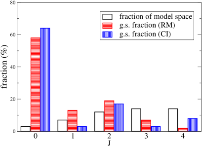
Figure 1: (color online) Distribution of ground state quantum numbers for eight neutrons in the $1p$-$0f$ shell. Empty bars are the fraction of states in the model space with a given $J$, horizontally striped (red) bars are the fraction of ground states with a given $J$ predicted by a random matrix (RM) model, and vertically striped (blue) bars are fraction of ground states with a given $J$ from configuration-interaction (CI) diagonalizations of an ensemble of random two-body Hamiltonian in a shell-model basis.

I can approximately correct both deficiencies. First, following standard results on matrices with Gaussian-distributed matrix elements RM , I let

$$\sigma_{J}^{\mathrm{eff}}=\sqrt{N_{J}}\sigma_{J}$$ (10)

be the width of the subspace of states with angular momentum $J$. Then, for each $J$, I simply create $N_{J}$ energies via a random Gaussian distribution of width $\sigma_{J}^{\mathrm{eff}}$, and ultimately determine the fraction of ground states with angular momentum $J$.

Finally, I compare against a variety of concrete simulations via configuration-interaction calculations, that is, diagonalizing the Hamiltonian for fixed numbers of particles in finite single-particle spaces. Figure 1 shows the case of eight fermions (neutrons) in the $1p_{1/2}$-$1p_{3/2}$-$0f_{5/2}$-$0f_{7/2}$ shell-model space (which in nuclear physics corresponds to ⁴⁸Ca with an inert ⁴⁰Ca core), while Table 1 considers two more cases, eight identical fermions in a $j=21/2$ shell, and six bosons in the interacting boson model (IBM) IBM .

For each of these many-body systems I take an ensemble of rotationally invariant, two-body but otherwise random interactions (typically a few thousand cases), and tabulate the fraction $f_{\mathrm{CI}}$ of states that have a given angular momentum $J$. This should be compared with the native fraction of states with that $J$ in each many-body space, $f_{\mathrm{space}}=N_{J}/N_{\mathrm{tot}}$ ($N_{\mathrm{tot}}$ is the total dimension of the many-body space), and as noted originally the fraction with $J=0$ is dramatically enhanced.

Table 1: Ground state quantum numbers for single-species systems, comparing the percentage of ground states of a given $J$ for configuration-interaction simulations ($f_{\mathrm{CI}}$) against the percentage computed using the simple random-matrix model ($f_{\mathrm{RM}}$) described in the text. As input, $f_{\mathrm{space}}$ is the fraction of the states with a given $J$ in the CI model space. The two cases are 8 fermions in a $j=21/2$ shell, and the $N=7$ interacting boson model (IBM).

$(21/2)^{8}$					IBM, $N=7$
$J$	$f_{\mathrm{space}}$	$f_{\mathrm{RM}}$	$f_{\mathrm{CI}}$		$J$	$f_{\mathrm{space}}$	$f_{\mathrm{RM}}$	$f_{\mathrm{CI}}$
0	0.4	33	55		0	11	81	55
1	0.5	0.2	0		1	(no states)
2	1	9	7		2	17	14	13
3	1	3	0.2		3	6	0.1	0.08
4	2	11	2		4	17	4	4

I also compare with the fraction of ground states with a given $J$ predicted by my simple random matrix picture, $f_{\mathrm{RM}}$. The only input are the dimensions $N_{J}$ and the universal variances computed in (9) and used in (10).

For such a simple picture, the random matrix model yields qualitatively excellent results, generally predicting the enhancement or suppression of different $J$s in the CI simulations relative to the native fractions $f_{\mathrm{space}}$. In particular, not only does the RM model successfully predict an enormous enhancement of $J=0$ in the ground state, it predicts a mild enhancement of $J=2$.

This analysis suggests the predominance of angular-momentum zero ground states is primarily a function of the width of the angular-momentum-projected many-body Hamiltonian; furthermore, the width is largely decoupled from the microphysics, instead depending only on the projection integrand (9) and on the dimensionality of subspaces with good quantum numbers. The simplicity and decoupling from the microphysics may be why the phenomenon is so robust and so universal.

So far I have only considered angular momentum. Yet in nature, nuclei with even numbers of protons and even numbers of neutrons always have $J=0$ ground states while those with odd numbers of protons and odd numbers of neutrons often do not, and if one runs ensembles of configuration-interaction simulations with two-body interactions that conserve angular momentum and and isospin, this scenario is broadly reproduced: one gets a predominance of $J=0$ ground states for even-even cases but greatly reduced for odd-odd.

Table 2: Distribution of ground state angular momentum $J$ for systems with equal numbers of protons and neutrons, given as a percent for configuration-interaction simulations ($f_{\mathrm{CI}}$) against fraction in the simple random-matrix model ($f_{\mathrm{RM}}$). The columns marked ‘conserved’ means isospin consevation was enforced, while for those marked ‘broken’ isospin was maximally broken. The single-particle model spaces are $1s$-$0d$ or $(sd)$ and $1p$-$0f$ or $(pf)$.

	conserved				broken
$J$	$f_{\mathrm{space}}^{T=0}$	$f_{\mathrm{space}}^{T=1}$	$f_{\mathrm{RM}}$	$f_{\mathrm{CI}}$	$f_{\mathrm{space}}$	$f_{\mathrm{RM}}$	$f_{\mathrm{CI}}$
$(sd),Z=N=3$
0	0.8	1.6	42	15	3.6	72	32
1	2.5	4.3	32	34	10	16	31
2	3.5	6.4	17	9	15	10	14
3	4.2	7.3	7	26	17	2	15
4	4.1	7.2	0.5	1.6	16	.1	4
$(pf),Z=N=3$
0	0.7	1.2	41	11	2.6	66	28
1	2.1	3.4	27	36	7.6	16	26
2	3.0	5.2	19	7	11	13	16
3	3.8	6.2	11	23	13	3	15
4	3.9	6.6	2	2	14	0.5	3

I now generalize the above simple model, and consider widths that depend upon both total angular momentum $J$ and total isospin $T$. If $N_{JT}$ is the dimension of a CI space with fixed $J$, $T$, then let the width be

$$\sigma^{\mathrm{eff}}_{JT}=\sqrt{N_{JT}}\sigma_{J}\sigma_{T}$$ (11)

where $\sigma_{T}$ is also taken from (9).

Table 2 shows the dimensions for several proton-neutron cases, both for fixed $J$, $T$ and for fixed $J$ alone, as well as the random matrix prediction for the fractions $f_{JT}$ and $f_{J}$. For even-even cases (not shown to save space), there is little difference, but for odd-odd, breaking isospin dramatically enhances the fraction of $J=0$ ground states. This can be considered a prediction of the simple random matrix model. The results can be traced directly to the subspace dimensions (here $f_{\mathrm{space}}$). Specifically, as one goes from isospin breaking to isospin conserving, a smaller fraction of $J=0$ states go to $T=0$ than do $J=1$, and the relative decrease of dimensionality of $J=0,T=0$ makes the difference.

I include the results of an ensemble of CI simulations, which verify the qualitative predictions of the random matrix model. While that quantitative agreement is significantly less than for the single-species case, the qualitative trends do agree.

In computing (9), I assumed each $\mathbf{F}(\omega)$ to be uncorrelated, so that the widths add incoherently. Suppose instead that that $\mathbf{F}(\omega)$ and $F(\omega^{\prime})$ are correlated, with a correlation length $\gamma$; then the width (9) becomes

$$4\pi^{2}\bar{\sigma}^{2}\int_{0}^{\pi}d\omega\int_{0}^{\pi}d\omega^{\prime}P_{J}(\cos\omega)\sin\omega P_{J}(\cos\omega^{\prime})\sin\omega^{\prime}$$

$$\times\exp\left(-|\omega-\omega^{\prime}|/\gamma\right).$$ (12)

In the limit $\gamma\rightarrow\infty$, which corresponds for a perfectly correlated, i.e. constant, $\mathbf{F}$ this vanishes for $J>0$. Fig. (2) shows how the fraction of ground states with $J$ varies with correlations length $\gamma$, for the case of ²⁴Mg.

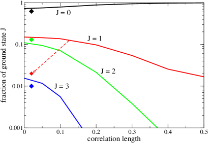
Figure 2: (color online) Fraction of ground states with angular momentum $J$ as a function of the correlation length (see Eq. 12), for $N=Z=4$ in the $sd$ shell. Diamonds correspond to the TBRE result; only the $J=1$ is shifted significantly, see dashed arrow.

Even if $\mathbf{F}(\omega)$ are not correlated, the $\mathbf{h}_{J}$ still have correlations because $\int P_{J}(\cos\omega)P_{J^{\prime}}(\cos\omega)\sin^{2}\omega d\omega\neq 0$; this correlation was found via a much more complicated prior analysis PW04 . One immediate result follows from the integral: while $J=0$ is correlated with all even $J$, it is not correlated with odd $J$. Further consequences will be pursued in future work.

In summary, detailed quantum many-body simulations using ensembles of random interactions have shown surprising trends, most notably the predominance of angular momentum $J=0$ in the ground state. To address this question, I have argued how one can project random matrices with good quantum numbers. Using only simple, universal integrals and the dimensionality of subspaces with good quantum numbers, I can qualitatively reproduce the features of ensembles of many-body systems. In particular I find an dominance of $J=0$ for the ground state, although I reproduce other trends as well. When I further consider systems with two species (protons and neutrons) the random matrix model predicts, and CI simulations confirm, that the subspace dimensions of isospin-conserving systems suppresses $J=0$ ground states in odd-$Z$, odd-$N$ systems.

The results of the model are qualitative, not quantitative. On the other hand, the effectiveness of the qualitative results for a broad variety of cases suggests that some properties of many-body systems are founded not in detailed microphysics but on simple properties, specifically projection integrals and the relative dimensions of subspaces with good quantum numbers.

The U.S. Department of Energy supported this investigation through grant DE-FG02-96ER40985.

References

- (1) T. A. Brody, J. Flores, J. B. French, P. A. Mello, A. Pandey, and S. S. M. Wong, Rev. Mod. Phys. 53, 385 (1981); M. L. Mehta, Random Matrices, 2nd ed. (Academic Press, Boston, 1991).
- (2) A. Bohr and B. R. Mottelson, Nuclear Structure, Vol II (W. A. Benjamin, Inc., Boston, 1975).
- (3) I. Talmi, Simple Models of Complex Nuclei (Harwood Academic Publishers, Chur
- (4) C. W. Johnson, G. F. Bertsch, and D. J. Dean Phys. Rev. Lett. 80, 2749 (1998).
- (5) V. Zelevinsky and A. Volya, Phys. Rep. 391, 311 (2004).
- (6) Y. M. Zhao, A. Arima, and N. Yoshinaga, Phys. Rep. 400, 1 (2004).
- (7) C. W. Johnson, Rev. Mex. Fis. 45 suppl. 2, 25 (1999).
- (8) R. Bijker and A. Frank, Phys. Rev. Lett. 84, 420 (2000).
- (9) A. Volya, Phys. Rev. Lett. 100, 162501 (2008).
- (10) K. K. Mon and J. B. French, Ann. Phys. (N.Y.) 95, 90 (1975).
- (11) R. Bijker, A. Frank, and S. Pittel, Phys. Rev. C 60, 021302 (1999)
- (12) T. Papenbrock and H. A. Weidenmüller Phys. Rev. Lett. 93, 132503 (2004); Phys. Rev. C 73, 014311 (2006).
- (13) D. Mulhall, A. Volya, and V. Zelevinsky, Phys. Rev. Lett. 85, 4016 (2000)
- (14) F. Iachello and A. Arima, The Interacting Boson Model (Cambridge University Press, Cambridge, 1987).