Finite-time quantum-to-classical transition for a Schrödinger-cat state

Abstract

The transition from quantum to classical, in the case of a quantum harmonic oscillator, is typically identified with the transition from a quantum superposition of macroscopically distinguishable states, such as the Schrödinger-cat state, into the corresponding statistical mixture. This transition is commonly characterized by the asymptotic loss of the interference term in the Wigner representation of the cat state. In this paper we show that the quantum-to-classical transition has different dynamical features depending on the measure for nonclassicality used. Measures based on an operatorial definition have well defined physical meaning and allow a deeper understanding of the quantum-to-classical transition. Our analysis shows that, for most nonclassicality measures, the Schrödinger-cat state becomes classical after a finite time. Moreover, our results challenge the prevailing idea that more macroscopic states are more susceptible to decoherence in the sense that the transition from quantum to classical occurs faster. Since nonclassicality is a prerequisite for entanglement generation our results also bridge the gap between decoherence, which is lost only asymptotically, and entanglement, which may show a sudden death. In fact, whereas the loss of coherences still remains asymptotic, we emphasize that the transition from quantum to classical can indeed occur at a finite time.

I Introduction

Ever since the early days of quantum theory the gap between our classical everyday reality and the quantum mechanical laws that govern the microscopic world has been acknowledged. The Schröodinger cat gedanken experiment, in which a real cat is cleverly put in a superposition of being alive and dead at the same time, illustrates the seemingly paradoxical conclusions arising from the application of quantum principles to macroscopic objects Schrodinger35 .

The prevailing explanation of the emergence of the classical realm from the quantum is environment induced decoherence (EID) Zurek91 ; Paz93d . According to the EID description the reason why macroscopic quantum superpositions are not observed in the classical world is the presence of the environment, which couples to all systems and effectively monitors quantum superpositions, inducing a collapse to the corresponding statistical mixture of classical-like states (pointer states). Experiments observing the quantum-to-classical transition, for Schrödinger cat-like states of both light and massive particles, have been performed, e.g., in the context of cavity QED and trapped ions, respectively Wineland96b ; Haroche96 ; Haroche08 .

Quantum superpositions of macroscopically (or mesoscopically) distinguishable states are sometimes called Schrödinger-cat states, in the spirit of the original Schrödinger’s thought experiment. Typically, decoherence of such a quantum superposition state that leads to a statistical mixture, is identified with the transition from quantum to classical, i.e., with the loss of the quantum features initially possessed by the cat state Zurek91 . According to one of the earliest definitions, a state is classical if it can be expressed as a statistical mixture of coherent states, i.e., if the $P$ function Glauber63 ; Sudarhsan63 ; Glauber65 ; Glauber69 of the state is a positive, well-defined probability distribution Glauber65 . Although examples of nonclassical states in line with this original definition exist Vogel08 , the $P$ function can also be highly singular making its reconstruction very demanding. Different definitions and criteria for nonclassical states have been proposed in the literature Lee91 ; Barnett95 ; Klyshko96 ; Vogel00 ; Vogel02 ; Lewenstein05 ; Casamiglia05 ; Egger97 , also for multimode fields ths09 ; mir10 ; sol10 ; bri11 , and the decoherence process has been analyzed extensively S1 ; S2 . The different approaches are not equivalent, so the complete characterization of nonclassical states, in particular a measurable criterion that is both necessary and sufficient, does not exist, except for pure states Vogel02 . Besides their fundamental importance, nonclassicality criteria are of key relevance also for quantum technologies. Creating and revealing nonclassical states, e.g., is often a prerequisite to generate entanglement for quantum information purposes in all-optical setups Knight02 ; Wang02 .

In this paper we consider five different definitions of nonclassicality for a single mode of the quantum harmonic oscillator, paying special attention to their physical meaning. We use these definitions to study the quantum-to-classical transition, i.e., the dynamics of a Schrödinger-cat state in presence of a dissipative environment inducing decoherence. The nonclassicality indicators we deal with are: the peak of the interference fringes of the Wigner function, the negativity of the Wigner function, Vogel’s noncalssicality criterion Vogel00 , the nonclassical depth Lee91 ; Barnett95 , and the Klyshko criterion Klyshko96 ; DAriano99 .

As opposed to the definition based on the fringe visibility of the Wigner function, which is the most widely used when describing the quantum-to-classical transition, the other four criteria offer some advantages. These definitions, indeed, have an operatorial interpretation, connecting the transition process to a measurable physical property. The interference fringes, on the contrary, are constructed mathematically assuming the full knowledge of the quantum state. In practice, however, any technique for quantum state estimation, including tomographic approaches, leads to a reconstruction of the density matrix within some confidence interval, so that the amount of nonclassicality is crucially influenced in a nonlinear way by the precision of the reconstruction technique LNP .

We find that, according to all the operatorial definitions, the quantum-to-classical transition occurs at a finite time rather than following an exponential decay, in accordance with the results found in Refs. JPADiosi ; ActaDiosi ; Marian for the nonclassical depth and the negativity of the Wigner function. It is worth noting that, contrarily to entanglement, which is defined independently of the entanglement measure used, the concept of nonclassicality or quantumness of the state does depend on the nonclassicality criterion used. More precisely, even if for mixed states different entanglement measures may give different numerical values, they all agree on the minimum zero value indicating disentanglement. Therefore, entanglement sudden death does not depend on the specific measure of entanglement chosen. On the contrary, as we will see, the loss of nonclassicality does depend on the criterion used to define nonclassicality. However, all operatorial definitions of nonclassicality show a similar behavior reinforcing the idea that the initial cat state loses its quantum character after a finite time, which we can identify with the maximum over the times the cat state becomes classical according to the different criteria.

We also study how the transition depends on the separation between the two coherent states of the initial superposition, finding that the dependence of the decoherence time from the separation, and therefore from the size of the cat state, is not at all trivial and can be counterintuitive. It is widely believed, indeed, that the more macroscopic the initial cat state is, the faster is the quantum-to-classical transition. This is indeed true for the fringe visibility criterion but, as we will see, using other criteria the situation changes drastically.

The paper is organized in the following way. In Section II we introduce the initial Schrödinger-cat state and the dynamics driving the transition. In Sec. III we introduce the five different nonclassicality conditions, we derive their environment-induced dynamics and, hence, we single out and compare the characteristic features of the quantum-to-classical transition, according to each definition. Finally, in Sec. IV we present concluding remarks and sum up the results.

II The system

Let us consider a quantum harmonic oscillator initially prepared in a superposition of coherent states with opposite phases, i.e., in the so-called Schrödinger-cat state,

$$|\Psi_{cat}\rangle=\frac{|\alpha\rangle+|-\alpha\rangle}{\sqrt{\cal N}}$$ (1)

where $|\alpha\rangle$ denotes a coherent state and

$$\mathcal{N}=2[1+\mathrm{exp}(-2|\alpha|^{2})]\,,$$

is the normalization constant. For the sake of simplicity we will assume amplitude $\alpha$ real throughout the paper. We then assume that the oscillator interacts with a bosonic bath of oscillators at thermal equilibrium at temperature $T$. In the Born-Markov approximation, and in the interaction picture, the evolution of the system is governed by the master equation

$$\frac{d\rho(t)}{dt}= \,\gamma(n+1)\big{[}2a\rho(t)a^{\dagger}-a^{\dagger}a\rho(t)-\rho(t)a^{\dagger}a\big{]}$$ (2)

$$+\gamma n\big{[}2a^{\dagger}\rho(t)a-aa^{\dagger}\rho(t)-\rho(t)aa^{\dagger}\big{]}\,,$$

where $\rho$ is the density matrix of the quantum harmonic oscillator, $\gamma$ the damping rate, $a$ and $a^{\dagger}$ the annihilation and creation operators and $n$ the mean occupation number of the thermal bath.

All the nonclassicality criteria that we will use in the paper are based on the quasiprobability distributions associated to quantum states. These are the quantum analogs of the classical distribution functions so, broadly speaking, any deviation from a classical probability distribution is considered as a sign of nonclassicality. The normalized quasiprobability distributions associated to the density matrix $\rho$ are defined as the Fourier transforms of the $s$-parametrized characteristic functions $\chi(\xi,s)$ Glauber69 ; Barnett95

$$W(\alpha,s)=\int\frac{d^{2}\xi}{\pi}\,\mathrm{e}^{\alpha\xi^{*}-\alpha^{*}\xi}\,\chi(\xi,s),$$ (3)

where

$$\chi(\xi,s)=\mathrm{Tr}[\rho\,\mathrm{e}^{\xi\hat{a}^{\dagger}-\xi^{*}\hat{a}}]\,\mathrm{e}^{\frac{1}{2}s|\xi|^{2}}\,.$$ (4)

The familiar $P$ function, Wigner function and Husimi $Q$ function are obtained by choosing $s=1$, $0$ and $-1$, respectively. These distribution functions correspond to normal, symmetric, and antinormal ordering of the creation and annihilation operators, respectively, and they can be easily obtained from one another via convolution, i.e., for $\tilde{s}<s^{\prime}$, one has

$$W(\alpha,\tilde{s}) =W(\alpha,s^{\prime})\star G(s^{\prime}-\tilde{s},\alpha)$$

$$=\int d^{2}\beta\,W(\beta,s^{\prime})\,G(s^{\prime}-\tilde{s},\alpha-\beta)\,,$$ (5)

where

$$G(\kappa,\alpha)=\frac{2}{\pi\kappa}\,\mathrm{exp}\left(-2\,\frac{|\alpha|^{2}}{\kappa}\right)$$ (6)

Different distributions can be found useful for different tasks. The Wigner function is often used to characterize nonclassicality because it is bounded from above allowing experimental measurements. It is well known, however, that defining nonclassicality in terms of the properties of different quasiprobability distributions, e.g., the $P$ function or Wigner function, does not yield equivalent results. The quantum-to-classical transition has been studied previously by monitoring the time evolution of the interference peak in the Wigner function representation Zurek91 . We include this approach in our study, and compare it to four other possible ways to characterize the quantum-classical border. Each approach has a different physical interpretation, with different strengths and weaknesses. In the next section, we analyze such differences in an effort to obtain insight into the emergence of classicality. To this aim we consider the dynamics of different nonclassicality measures and study the time at which the initial nonclassical state evolves into a classical one and the dependence of such time from the relevant system parameters.

III Loss of nonclassicality of the Schrödinger-cat state

Monitoring the dynamics of the cat state as it evolves into a statistical mixture is a natural way of studying the quantum-to-classical transition since the initial superposition is not an element of the macroscopic, classical reality, whereas the final statistical mixture of minimum uncertainty coherent states is, the latter states being the closest equivalent of a classical point in phase space. The precise way of characterizing the transition leads to different dynamical features and interpretations. In the following we study analytically the time evolution of the peak of the interference fringes of the Wigner function, the nonclassicality depth, the negativity of the Wigner function, Vogel nonclassicality criterion and the Klyshko criterion.

III.1 Peak of the interference fringe

A common way of monitoring the quantum to classical transition by using the Wigner function is based on the time evolution of the highest point of the interference term, characterizing the Schrödinger-cat state of Eq. (1). Such a term is an indicator of the quantumness of the superposition and hence its disappearance signals the transition to a classical mixture. The presence of the interference peak can be quantified via the fringe visibility function

$$F(\alpha,t) \equiv\mathrm{exp}(-A_{int})$$

$$=\frac{1}{2}\frac{W_{I}(\beta,t)|_{\mathrm{peak}}}{[W^{(+\alpha)}(\beta,t)|_{\mathrm{peak}}W^{(-\alpha)}(\beta,t)|_{\mathrm{peak}}]^{1/2}},$$ (7)

where $W_{I}(\beta,t)|_{\mathrm{peak}}$ is the value of the Wigner function at $\beta=(0,0)$ and $W^{(\pm\alpha)}(\beta,t)|_{\mathrm{peak}}$ are the values of the Wigner function at $\beta=(\pm\alpha,0)$, respectively. This is a widely used signature for the emergence of classicality Paz93d and it has been experimentally monitored as well Haroche96 ; Wineland96b ; Haroche08 . The time evolution of the fringe visibility for an oscillator initially prepared in a cat state and then evolving in a noisy channel reads as follows

$$F(\alpha,\tau)=\mathrm{exp}\left[-2\alpha^{2}\left(1-\frac{C_{t}^{2}}{1+2D_{t}}\right)\right],$$ (8)

where

$$C_{t}=\mathrm{e}^{-\gamma t}\qquad D_{t}=n(1-\mathrm{e}^{-2\gamma t})\,.$$ (9)

The time evolution of the same quantity without the Markovian approximation (i.e., taking into account the memory effects of structured reservoirs) has been studied in Paavola10 .

As we can see from (8), the fringes disappear asymptotically. If one then takes the peak of the interference fringe as an indicator of nonclassicality, the quantum-to-classical transition does not occur at a finite time. No known operatorial expression, however, can be given for the fringe visibility. Therefore it can be seen as a calculational tool to describe decoherence, with no obvious observable associated to it. Moreover, characterizing decoherence in this way requires the full knowledge of the state density matrix, obtained with complete tomographic measurements.

The dependence of the decoherence rate on the initial separation can be seen from Eq. (8). This quantity is proportional to $\alpha^{2}$, resulting in faster decoherence for more macroscopic initial cat states. The explanation of the emergence of the classical world from the quantum one, according to environment induced decoherence, is heavily based on this observation. More macroscopic states loose their quantumness faster, and that is why we do not see any of the bizarre effects predicted by quantum theory in our daily ”macroscopic” life. However, as we will see in the following subsections, this conclusion is strongly dependent on the nonclassicality critierion considered, and therefore cannot be used to corroborate the main traits of the quantum-to-classical transition, such as the dependence of the decoherence time on the size of the system.

III.2 Nonclassical depth

Let us now focus on the nonclassical depth that can be obtained from the properties of the generalized distribution functions introduced in Sec. II. The nonclassical depth was first introduced by Lee Lee91 and, in a slightly different form, by Lütkenhaus and Barnett Barnett95 some years later.

The starting point is the $s$-parametrized quasidistribution function given by Eq. (II), with $s$ a continuous parameter. Setting $s^{\prime}=1$ in Eq. (II) one obtains an expression giving $W(\alpha,s)$ as a convolution of the $P$ function,

$$W(\alpha,s)=P(\alpha)\star G(1-s,\alpha)$$ (10)

Note that, for $s=1,0,-1$, $W(\alpha,s)$ coincides with the $P$, $W$ an $Q$ functions, respectively. While the $P$ and the $W$ functions cannot be generally considered proper distribution function, the $Q$ function can, being always positive and regular. However, we note in passing that, even if the $Q$ function is always positive, its marginals are only approximate (broadened) position and momentum variables. Hence its use as an indicator of classicality should be considered with care, as discussed in some detail, e.g., in Ref. Milburn86 .

The nonclassical depth of a given state is

$$\eta=\frac{1}{2}(1-\bar{s})$$

where $\bar{s}$ is the largest value of $s$ for which $W(\alpha,s)$ is positive. For pure states $0\leq\eta\leq 1$, while mixed states can have any value of $\eta<1$. It was shown in Ref. Barnett95 that for all pure states other than coherent squeezed states the nonclassical depth is $\eta=1$, squeezed states have $0\leq\eta\leq 1/2$, while coherent state have $\eta=0$, in accordance with the fact that they are the closest analogue to classical states for the quantum harmonic oscillator.

In order to study the dynamics of the nonclassical depth $\eta$, for the initial state of Eq. (1), we notice that the time evolution of the $P$ function, in presence of a dissipative thermal environment leading to the master equation (2), can be written in a form similar to Eq. (10). As we will see in the following, this allows us to single out an analytic expression for the instant of time $\tau_{P}$ which is an upper bound for the loss of nonclassicality. The solution to the master equation (2) can be written in terms of the normally ordered characteristic function $\chi(\xi,s=1)\equiv\Phi(\xi)$. Upon denoting by $\Phi_{0}(\xi)$ the characteristic function at $t=0$ (i.e., the one of the initial cat state) we have that the characteristic function at time $t$ is given by

$$\Phi_{t}(\xi)=\Phi_{0}(C_{t}\xi)\,\mathrm{exp}(-D_{t}|\xi|^{2}),$$ (11)

where the coefficients $C_{t}$ and $D_{t}$ are given in Eq. (9). From Eq. (3), with $s=1$, and Eq. (11) one obtains

$$P_{t}(C_{t}\alpha)=\frac{1}{C_{t}^{2}}\, \int\frac{d^{2}\xi}{\pi}\,\Phi_{0}(\xi)\,\mathrm{e}^{-\frac{D_{t}}{C_{t}^{2}}\,|\xi|^{2}+\alpha\xi^{*}-\alpha^{*}\xi}\,.$$ (12)

Remembering that the Fourier transform of a product of two functions is equal to the convolution of the two corresponding Fourier transforms, we can recast Eq. (12) in the form

$$C_{t}^{2}P_{t}(C_{t}\alpha) =P_{0}(\alpha)\star G(1-s_{t},\alpha)$$ (13)

$$\equiv W(\alpha,s_{t})\,,$$

with

$$s_{t}=1-2v_{t}\,,\qquad v_{t}=D_{t}/C_{t}^{2}.$$ (14)

Thus, the master equation (2) essentially turns the $P$ function of the initial state into the quasiprobability distribution function $W(\alpha,s)$ of the initial state. Indeed, at $t=0$, $s_{0}=1$ and the r.h.s. reduces to the $P$ function. As time increases $v_{t}$ increases and, correspondingly, $s_{t}$ decreases. An upper limit to the time at which the state becomes classical is therefore given by the time $t_{{\scriptscriptstyle P}}$ at which $s_{t_{P}}=-1$, since in this case the $P$ function of our initial state has become the $Q$ function, and therefore it is positive. Note that $t_{{\scriptscriptstyle P}}$ is an upper limit to the disappearance of nonclassicality. Since the evolved state is always a mixed state, indeed, $\bar{s}$ can be greater than $s_{t_{P}}$. It follows via Eq. (14) that the time $\tau_{\scriptscriptstyle P}=\gamma t_{{\scriptscriptstyle P}}$ is given by

$$\tau_{\scriptscriptstyle P}=\frac{1}{2}\mathrm{ln}\left(\frac{1}{n}+1\right)=\frac{\hbar\omega}{2k_{B}T},$$ (15)

in agreement with Marian et al. Marian , with $\omega$ the frequency of the harmonic oscillator, $k_{B}$ the Boltzmann constant, and $T$ the reservoir temperature. After this time the state is classical, therefore $\tau_{{\scriptscriptstyle P}}$ quantifies the lifetime of the nonclassical Schrödinger-cat state. Note that this time is always finite for any $n\neq 0$, in this sense we can talk about finite-time transition from quantum to classical for the Schrödinger-cat state. For smaller and smaller values of the reservoir temperature, the lifetime of the cat state increases.

It is worth stressing that $\tau_{{\scriptscriptstyle P}}$ is an upper bound to the nonclassical depth, and therefore to the quantum-to-classical transition time, for any initial nonclassical state since it corresponds to the time at which the $P$ function of any initial state has evolved into a positive distribution function, i.e., the $Q$ function, and since at all times $t>0$ the evolved state is a mixed state.

III.3 Negativity of the Wigner function

The negativity of the Wigner function has been used widely as a nonclassicality definition, mostly due to the fact that the Wigner function is never singular, as opposed to the $P$ function, and therefore it is possible to reconstruct it in an approximate way through quantum homodyne tomography. Recently it was shown that measuring merely two conjugate variables, instead of performing full state tomography, is sufficient to observe the negativity of the Wigner function in a certified, error-free way Mari10 .

In the previous section we have seen that the master equation describing the system dynamics, given by Eq. (2), essentially transforms the $P$ function of the initial state into the generalized quasidistribution function $W(\alpha,s)$ of the initial state, according to Eq. (12). This equation describes also the evolution of the initial Wigner function since at a certain time $\bar{t}$, $s_{\bar{t}}=0$ and the dissipative channel has transformed the initial $P$ function of our state into the $W$ function. It follows straightforwardly that, an upper limit to the disappearance of negativity of the Wigner function is given by the time $t_{\scriptscriptstyle W}$ such that $s_{t_{\scriptscriptstyle W}}=0$, i.e., following Eq. (14),

$$\tau_{\scriptscriptstyle W}=\gamma t_{\scriptscriptstyle W}=\frac{1}{2}\mathrm{ln}\left(\frac{1}{2n}+1\right)\,.$$ (16)

Note that, for high $T$-reservoirs, i.e., for $n\gg 1$, $\tau_{\scriptscriptstyle W}\approx 1/4n$ and $\tau_{\scriptscriptstyle P}\approx 1/2n=2\tau_{\scriptscriptstyle W}$, indicating that the negativity of the Wigner function disappears faster than the nonclassical depth.

III.4 Vogel criterion

III.4.1 1st order nonclassicality criterion

The Vogel nonclassicality criterion states that a state is nonclassical if there exist values of $u$ and $v$ such that

$$|\Phi(\xi)|>1$$ (17)

for the normally ordered characteristic function, where $\xi=u+iv$. In terms of the symmetrically ordered characteristic function $\chi(\xi,0)$ the condition reads

$$|\chi(\xi,0)|>\chi_{0}(\xi,0)\equiv\mathrm{exp}\left(-\frac{1}{2}|\xi|^{2}\right)$$ (18)

where $\chi_{0}(\xi,0)$ is the characteristic function of the ground state of the system oscillator Vogel00 . It is worth noticing that the symmetric characteristic function can be directly measured via balanced homodyne detection. Formulating a criterion for nonclassicality in terms of the inequality (18) therefore means that complete state tomography is not anymore necessary to characterize the nonclassical status of a state. A single measurement satisfying inequality (18) is sufficient, and maintaining a stable relation between the local oscillator and the optical state becomes unnecessary Shapiro02 . This makes checking for the nonclassicality of a state much simpler compared to full state tomography. Experiments demonstrating the usefulness of the nonclassicality criterion in Eq. (18) have already been performed Shapiro02 .

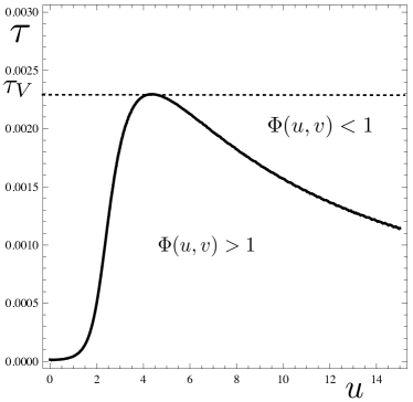
Figure 1: Vogel nonclassicality condition as a function of $\tau=\gamma t$ and $u$, for $v=0$, $n=100$ and $\alpha=2$. The solid line corresponds to $\Phi_{t}(u,0)=1$. The state is nonclassical in the area under the curve. The time $\tau_{\scriptscriptstyle V}$ is the time at which the state becomes classical.

However, some nonclassical states may not be captured by this definition, as demonstrated by Diósi in Ref. Diosi00 . This criterion is therefore sufficient but not necessary. The criterion was later generalized by Richter and Vogel to give necessary and sufficient conditions for nonclassicality Vogel02 . The new criterion consists of an infinite set of conditions, considerably affecting its practical usability. The original simple criterion of Eq. (18) is still extremely useful as it can reliably and with few measurements confirm an unknown quantum state as nonclassical. For the initial cat state of Eq. (1) the time evolution of the normally ordered characteristic function reads MQOB

$$\Phi_{t}(u,v) = \frac{2}{\mathcal{N}}\,e^{-D_{t}(u^{2}+v^{2})}\Big{[}\cos(2C_{t}\alpha v)$$ (19)

$$+ e^{-2\alpha^{2}}\cosh(2C_{t}\alpha u)\Big{]}.$$

Using Eq. (19), we have investigated numerically the time evolution of Eq. (17) in the high $T$ limit finding that, after a finite time, it is not satisfied anymore. Since $\Phi_{t}(u,v)\leq\Phi_{t}(u,0)$, we plot in Fig. 1 the contour line corresponding to $\Phi_{t}(u,0)=1$. This contour line indicates the transition from quantum to classical, according to Vogel first order nonclassicality criterion. The dashed line indicates the time $\tau_{\scriptscriptstyle V}(\alpha)$ after which the quantum property connected to the initially macroscopically separated cat state, namely the one described by condition (18), is lost.

III.4.2 Dependence on the size of the cat state

We now focus on the dependence of $\tau_{\scriptscriptstyle V}(\alpha)$ on the initial wave packet separation $\alpha$. In Fig. 2 we show how the contour line $\Phi_{t}(u,0)=1$, indicating the loss of nonclassicality, changes for increasing values of $\alpha$. In more detail, we vary $\alpha$ in unit step size from $1$ to $10$, corresponding to the curves from left to right. Interestingly, the time $\tau_{\scriptscriptstyle V}(\alpha)$ of loss of nonclassicality of the Schrödinger-cat state increases with the initial wave packet separation. This means essentially that the more macroscopic the initial state is, the longer it takes to become classical. This is in strong contrast with the usual picture of emergence of the classical world from the quantum world in terms of environment induced decoherence, according to which the more macroscopic the cat state is, the faster is the quantum-to-classical transition. Our results show that this is in fact only true for the peak of interference fringes but not for other nonclassicality indicators, such as the Vogel first order criterion.

Another interesting feature shown in Fig. 2 is that the time after which the nonclassicality condition (18) ceases to be satisfied seems to saturate, possibly indicating an upper bound for the onset of classicality for initially highly nonclassical states. In fact it is possible to calculate such an upper bound analytically noticing that for $\alpha\rightarrow\infty$ one has

$$\Phi_{t}(u,0) \approx e^{-D_{t}u^{2}}$$

$$+\frac{1}{2}e^{-D_{t}(|u|-\alpha C_{t}/D_{t})^{2}}e^{-\alpha^{2}(2-C_{t}^{2}/D_{t})}.$$ (20)

From the equation above one can easily prove that a necessary and sufficient condition for the state to be classical according to the first-order Vogel nonclassicality criterion, in the limit $\alpha\rightarrow\infty$, is given by the equation

$$C_{t}^{2}\leq 2D_{t}.$$ (21)

Note that Eq. (21) coincides with the equation defining the time for the loss of nonclassicality, $\tau_{\scriptscriptstyle W}$, in terms of the negativity of the Wigner function. Hence,

$$\tau_{\scriptscriptstyle V}(\alpha)\stackrel{{\scriptstyle\alpha\rightarrow\infty}}{{\longrightarrow}}\frac{1}{2}\ln\left(1+\frac{1}{2n}\right)\equiv\tau_{\scriptscriptstyle W}\,.$$ (22)

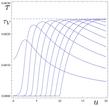
Figure 2: Vogel nonclassicality condition $\Phi_{t}(u,0)=1$ as a function of $\tau=\gamma t$ and $u$, for $v=0$, $n=100$ and initial separations $\alpha$ ranging from 1 to 10 (lines from left to right, respectively). The dashed line marks the saturation time $\tau_{\scriptscriptstyle V}(\alpha\rightarrow\infty)$ after which the state is classical.

III.4.3 2nd order nonclassicality criterion

The loss of nonclassicality, in the sense of $P$ function not being a probability density, is not guaranteed by the condition (17). Nonetheless, the use of Vogel first order nonclassicality criterion to characterize the quantumness of a state has some benefits. In most cases, indeed, it correctly identifies nonclassical states, the only known exception being the example given by Diósi in Diosi00 . Moreover, it is sufficiently simple to be of use in experiments and, in the context of cat states and quantum-to-classical transition, it can be used as a meaningful characterization of the dynamics since the initial state satisfies Eq. (17) but along the evolution the inequality becomes invalid and hence, the state classical. In other words, a property connected to the initially macroscopically separated cat state, namely the one described in Eq. (17), has been lost, and we choose to use this property as a characterization of the quantum-to-classical transition.

Although we argue that the nonclassicality criterion (17) could be used to indicate the finite-time quantum-to-classical transition, and do not aim to use in this paper the infinite set of nonclassicality conditions by Richter and Vogel Vogel02 , we have also numerically studied the time evolution of the second order criterion which, in terms of the normally ordered characteristic function, reads

$$|{\Phi_{1}}|^{2}+|{\Phi_{2}}|^{2}+|{\Phi_{12}}|^{2}-2\mathrm{Re}{|\Phi_{1}\Phi_{2}\Phi_{12}^{*}|}>1,$$ (23)

where $\Phi_{i}=\Phi(u_{1},v_{1})$ and $\Phi_{ij}=\Phi(u_{i}+u_{j},v_{i}+v_{j})$. We have verified that the finite-time quantum-to-classical transition of the cat state occurs also in second order but it takes a slightly longer time than in the case of the first order condition.

III.5 Klyshko criterion

The final nonclassicality criterion we are going to consider is based on the work of Klyshko Klyshko96 . It takes the form of an inequality involving terms from the photon number distribution of the mode under investigation. Since photon number distributions may be effectively reconstructed tomo ; pcount and in some cases also directly measured burle ; m , this method has a clear experimental advantage. Klyshko showed that an equivalence between a phase-averaged $P$ function,

$$F(r)=\int_{0}^{2\pi}\frac{d\phi}{2\pi}P(r\mathrm{e}^{i\phi}),$$ (24)

and an infinite set of inequalities concerning photon number probabilities $p(n)=\langle n|\hat{\rho}|n\rangle$ exists, providing a necessary and sufficient condition for nonclassicality in terms of negativity of $F(r)$. The simplest sufficient criterion for nonclassicality takes the form Klyshko96 ; DAriano99

$$B(n)\equiv(n+2)p(n)p(n+2)-(n+1)[p(n+1)]^{2}<0.$$ (25)

For $F(r)$ to be negative, it is sufficient that this condition is satisfied by just one non-negative integer number $n$. The photon number probabilities can be obtained from

$$p(n,t)=\frac{1}{\pi}\int du\,dv\,\Phi_{t}(u,v)\,\chi_{n}(u,v),$$ (26)

where $\Phi_{t}(u,v)$ is the characteristic function of the (evolved) cat state from Eq. (19) and $\chi_{n}(u,v)=\mathrm{exp}(-u^{2}-v^{2})L_{n}(u^{2}+v^{2})$ is the anti-normally ordered characteristic function of Eq. (4), with $s$=-1, for the Fock number state $|n\rangle$, $L_{n}(x)$ being the $n$-th Laguerre polynomials. For our initial cat state, the simplest condition showing the nonclassicality is provided by negativity of $B(1)$.

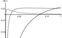
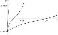
Figure 3: The Klyshko quantity $B(1)$ as a function of the rescaled time $\tau=\gamma t$ for different values of the thermal noise and different separation amplitude (left: $\alpha=2$, right:$\alpha=3$). Nonclassical states turn into classical ones at a threshold time $\tau_{\scriptscriptstyle K}$ depending on both the amplitude and the thermal noise. In both plots solid lines are for $n=1$, dashed for $n=10$ and dotted for $n=100$.

In Fig. 3 we show the time evolution of $B(1)$ for different values of the amplitude $\alpha$ and the thermal noise $n$. As it is apparent from the plot, all the states exhibit a crossing from quantum to classical state at a threshold time $\tau_{\scriptscriptstyle K}$ which is a decreasing function of the thermal noise. The effect of initial separation, i.e., the function $\tau_{\scriptscriptstyle K}(\alpha)$, is depicted in Fig. 4 for different values of the thermal noise. The nonclassicality condition $B(1)<0$ is satisfied in the gray areas of the plot, showing the transition time from quantum to classical as a function of the initial wave packet separation. We see that the classical domain is reached quite quickly for small and large amplitudes, with weak dependence on the thermal noise, whereas an optimum region of separation amplitudes exists ($\alpha\approx 2$) which maximizes the survival of nonclassicality and introduces a strong dependence on the thermal noise.

The behaviour of $B(n)$, for $n>1$, becomes increasingly difficult to obtain analytically. We have done some numerical comparisons and found indications that the nonclassicality thresholds obtained for higher order $B(n)$ are subsumed by that of $B(1)$. This was numerically confirmed for $B(2)$ and $B(3)$.

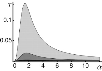
Figure 4: The nonclassicality condition $B(1)<0$ is satisfied in the gray areas of the plot showing the transition time from quantum to classical as a function of the initial wave packet separation. Here $\tau=\gamma t$, and (from larger to smaller areas) $n=1,10,100$. The border of each gray area individuates the function $\tau_{\scriptscriptstyle K}(\alpha)$.

The dependence of the Klyshko criterion on the initial separation $\alpha$ is qualitatively different from the ones predicted by all other criteria discussed in the paper. As can be viewed from Fig. 4, there exists a specific value, $\alpha\approx 2$, that maximizes the time of nonclassicality for the initial cat state. This is unique, since it implies that certain, arbitrary, cat states are favored, in terms of the endurance of quantumness. Actually, this is due to the structure of the quantity $B(1)$, which is built from the overlap of the cat state characteristic function with the characteristic functions of Fock states with small values of $n$, all localized in the proximity of the phase-space origin. This circumstance, together with the fact that higher order nonclassical tests seem to be subsumed by $B(1)<0$, suggest that the Klyshko criterion is not suitable to follow the time evolution of nonclassicality for highly separated superpositions.

IV Discussion and conclusions

In this paper we have addressed the problem of the quantum-to-classical transition by examining the loss of crucial quantum properties in an initial Schrödinger-cat state, which we identify with a quantum superposition of two coherent states with opposite phases. Under the influence of a dissipative environment the state decoheres and eventually reaches a state that can be considered purely classical, namely, a statistical mixture of the two coherent states.

We have shown that, depending on the measure of nonclassicality considered, the time at which one can say that the state has become classical, varies. In Table 1 we list the different methods that we have compared in the paper, along with the numerical value of the time threshold $\tau$ after which the nonclassicality is lost for a given value of $\alpha$ and of the bath temperature $T$. We also summarize the dependence of the threshold value on the separation between the components of the quantum superposition and on $T$. The only quantitatively different threshold time $\tau$, is related to the fringe visibility criterion, which gives an asymptotic transition from quantum to classical. All the other measures predict that the quantumness of the state is lost after a finite time, i.e., there exists a sudden transition from quantum to classical for the Schrödinger-cat state. It is notable that for the fringe visibility no known operatorial interpretation exists, as far as the authors are aware.

By contrast, the quadrature characteristic function used in Vogel nonclassicality criterion can be measured for freely propagating radiation modes, cavity-field modes Meystre91 and the quantized center-of-mass motion of a trapped ion in a harmonic potential Wallentowitz95 . This last methods offers an operatorial approach to the nonclassicality problem. It was shown in Ref. Wallentowitz95 that the full state information of the vibrational motion of a trapped ion can be obtained simply by monitoring the evolution of the ground state occupation probability in a long-living electronic transition. We stress once more, however, that Vogel criterion, as given by Eq. (18), does not capture all nonclassical states, as Diósi demonstrated in Diosi00 . However, since the criterion is satisfied for the initial cat states, it singles out a property that belongs to such superpositions. In this case the finite-time quantum-to-classical transition of the cat state coincides with the time at which the nonclassicality property associated to Vogel’s first order criterion is lost.

For the master equation (2), and for finite bath temperatures, there exists always a transition from quantum to classical, according to the original $P$ function criterion for nonclassicality. This can be seen from the nonclassical depth. Studying this quantity one sees that there exists always a specific time $t_{P}$ (or equivalently an amount of noise that needs to be added to the system) after which the $P$ function of the initial state evolves into a classical $Q$ function. The explicit expression of $\tau_{P}$, given by Eq. (15), suggests the conjecture that classicality emerges on a time scale inversely proportional to the effective temperature of the environment, for very general systems and environments. It is noteworthy in this definition that all pure initial states, apart from coherent squeezed states, have the same threshold time for the quantum-to-classical transition (or, equivalently, they can withstand the same amount of noise added before losing their quantumness).

The negativity of the Wigner function is another widely used indicator for nonclassicality. However, it is well known that this quantity is unable to identify all the states that are nonclassical according to the $P$ function (squeezed states are a prime example). The popularity of the Wigner function negativity stems from the fact that the Wigner function, unlike the $P$ function, can be measured with homodyne detection.

Finally, the Klyshko criterion, which expresses the positivity of the phase averaged $P$ function in terms of the moments of the photon number distribution, is the most sensitive of all the criteria discussed here. It has the advantage of being experimentally accessible since the photon number distribution, and in particular the probabilities needed to calculate $B(1)$, may be reliably measured even by an on/off detector pcount . On the other hand, this quantity does not appear suitable for superpositions of states with large separations.

The most important result of this paper is to challenge the current view regarding the quantum-to-classical transition due to environment induced decoherence. Indeed, it has been widely accepted that the more macroscopic the initial quantum superposition state is, the faster is the decoherence and, hence, the transition from quantum to classical. However, our results show that, for almost all the nonclassicality indicators, an increase in the initial wave packet separation does not necessarily increase the time after which decoherence has destroyed all nonclassical properties. The analysis of the Vogel and Klyshko criteria, e.g., shows that the dependence on $\alpha$ can be more complicated. In some cases, indeed, the transition time from quantum to classical can increase, instead of decreasing, with the separation between the components of the superposition.

What is conceptually interesting in our results is that they bridge the gap existing between decoherence and entanglement. Nonclassicality is a prerequisite for entanglement. However, the phenomenon of entanglement sudden death, discovered in 2001 Eberly02 , showed that entanglement can disappear completely after a finite time while decoherence, responsible for the loss of nonclassicality, decays only asymptotically Blatt . The comparison of the dynamical features of several nonclassicality measures clearly shows that, while the loss of quantum coherences is indeed asymptotic, the quantum properties present in the initial state, which are defined by the measure chosen, disappear after a finite time.

Table 1: Threshold time for quantum-to-classical transition according to different indicators of nonclassicality for $\alpha=2$ and $n=100$. The last two columns summarize the dependence of the threshold value on the cat state amplitude and on the mean occupation number of the thermal bath, i.e., on the temperature.

Nonclassicality measure		threshold time $\tau$		dependence on $\alpha$		dependence on $n$
Klyshko criterion		0.0019		$\tau$ is maximum for $\alpha\approx 2$		decreasing with $n$, see Fig. 4
Vogel criterion		0.0023		saturates with growing $\alpha$		decreasing with $n$
Negativity of $W(\alpha)$		0.0025		independent of $\alpha$		decreasing with $n$, see Eq. (16)
Negativity of $P(\alpha)$		0.0050		independent of $\alpha$		decreasing with $n$, see Eq. (15)
Fringe visibility		$\infty$		proportional to $\alpha^{2}$		still asymptotic, converges faster, see Eq. (8)

References

- (1) E. Schrödinger, Naturwissenschaften 23, 807, 823, 844 (1935); reprinted in english in Quantum Theory of Measurement, J. A. Wheeler and W. H. Zurek, Princeton University Press, (Princeton, NJ) 1983.
- (2) W. H. Zurek, Physics Today 44(10), 36 (1991).
- (3) J. P. Paz, S. Habib, and W. H. Zurek, Phys. Rev. D 47, 488 (1993).
- (4) C. Monroe, D. M. Meekhof, B. E. King, and D. J. Wineland, Science 272, 1131 (1996).
- (5) M. Brune, E. Hagley, J. Dreyer, X. Maitre, A. Maali, C. Wunderlich, J. M. Raimond, and S. Haroche, Phys. Rev. Lett. 77, 4887 (1996).
- (6) S. Deleglise, I. Dotsenko, C. Sayrin, J. Bernu, M. Brune, J. M. Raimond, and S. Haroche Nature 455, 510 (2008).
- (7) R. J. Glauber, Phys. Rev. 131, 2766 (1963).
- (8) E. C. G. Sudarshan, Phys. Rev. Lett. 10, 277 (1963).
- (9) U. M. Titulaer and R. J. Glauber, Phys. Rev. 140, B676 (1965).
- (10) K. E. Cahill, R. J. Glauber, Phys. Rev. 177, 1882 (1969).
- (11) T. Kiesel, W. Vogel, V. Parigi, A. Zavatta and M. Bellini, Phys. Rev. A 78, 021804R (2008).
- (12) C. T. Lee, Phys. Rev. A 44, R2775 (1991).
- (13) N. Lütkenhaus and S. M. Barnett, Phys. Rev. A 51, 3340 (1995).
- (14) D. N. Klyshko, Phys. Lett. A 213, 7 (1996).
- (15) W. Vogel, Phys. Rev. Lett. 84, 1849 (2000).
- (16) Th. Richter and W. Vogel, Phys. Rev. Lett. 89, 283601 (2002).
- (17) J. K. Korbicz, J. I. Cirac, J. Wehr, and M. Lewenstein, Phys. Rev. Lett. 94, 153601 (2005).
- (18) J. K. Asbóth, J. Calsamiglia, and H. Ritsch, Phys. Rev. Lett. 94, 173602 (2005).
- (19) R. Egger, H. Grabert, and U. Weiss, Physi. Rev. E 55, R3809 (1997).
- (20) I. P. Degiovanni, M. Genovese, V. Schettini, M. Bondani, A. Andreoni, M. G. A. Paris, Phys. Rev. A 79, 063836 (2009).
- (21) A. Miranowicz, M. Bartkowiak, X. Wang, Y. X. Liu, and F. Nori Phys. Rev. A 82, 013824 (2010).
- (22) J. Solomon Ivan, S. Chaturvedi, E. Ercolessi, G. Marmo, G. Morandi, N. Mukunda, and R. Simon, arXiv:1009.6104v1
- (23) G. Brida, M. Bondani, I. P. Degiovanni, M. Genovese, M. G. A. Paris, I. Ruo Berchera, and V. Schettini, Found. Phys. 41, 305 (2011).
- (24) A. Serafini, M. G. A. Paris, F. Illuminati, and S. De Siena, J. Opt. B: Quantum Semiclass. Opt. 7 R19 R36 (2005).
- (25) A. Serafini, S. De Siena, F. Illuminati, and M. G. A. Paris, J. Opt. B: Quantum Semiclass. Opt. 6 S591 S596 (2004).
- (26) M. S. Kim, W. Son, V. Buzek, and P. L. Knight, Phys. Rev. A 65, 032323 (2002).
- (27) Wang Xiang-bin, Phys. Rev. A 66, 024303 (2002).
- (28) G. M. D’Ariano, M. F. Sacchi, and P. Kumar, Phys. Rev. A 59, 826 (1999).
- (29) Quantum State Estimation M. G. A. Paris and J. Rehacek Eds., Lecture Notes in Physics 649, (Springer, Heidelberg, 2004).
- (30) L. Diósi, J. Phys. A 35, 2675 (2002).
- (31) L. Diósi, Acta Phys. Hung. B 20, 29 (2004).
- (32) P. Marian and T. A. Marian, Eur. Phys. J. D 11, 257 (2000).
- (33) J. Paavola and S. Maniscalco, Phys. Rev. A 82, 012114 (2010).
- (34) G. J. Milburn, Phys. Rev. A 33, 674 (1986).
- (35) A. Mari, K. Kieling, B. M. Nielsen, E. S. Polzik, and J. Eisert, Phys. Rev. Lett. 106, 010403 (2011).
- (36) A. I. Lvovsky and J. H. Shapiro, Phys. Rev. A 65, 033830 (2002).
- (37) L. Diósi, Phys. Rev. Lett. 85, 2841 (2000).
- (38) Methods in Theoretical Quantum Optics, S. M. Barnett and P. M. Radmore, Oxford University Press (Oxford), 1997.
- (39) M. Munroe, D. Boggavarapu, M. E. Anderson, and M. G. Raymer, Phys. Rev. A 52, R924 (1995); Y. Zhang, K. Kasai, and M. Watanabe, Opt. Lett. 27, 1244 (2002).
- (40) A. R. Rossi, S. Olivares, M. G. A. Paris, Phys. Rev. A 70, 055801 (2004); G. Zambra, A. Andreoni, M. Bondani, M. Gramegna, M. Genovese, G. Brida, A. Rossi, and M. G. A. Paris, Phys. Rev. Lett. 95, 063602 (2005).
- (41) G. Zambra, M. Bondani, A. S. Spinelli, and A. Andreoni, Rev. Sci. Instrum. 75, 2762 (2004).
- (42) A. Fukasawa, J. Haba, A. Kajeyama, H. Nakazawa, and M. Suyama, IEEE Trans. Nucl. Sci. 55, 758 (2008).
- (43) M. Wilkens and P. Meystre, Phys. Rev. A 43, 3832 (1991).
- (44) S. Wallentowitz and W. Vogel, Phys. Rev. Lett. 75, 2932 (1995).
- (45) T. Yu and J. H. Eberly, Phys. Rev. Lett. 93, 140404 (2004).
- (46) Julio T. Barreiro, Philipp Schindler, Otfried G hne, Thomas Monz, Michael Chwalla, Christian F. Roos, Markus Hennrich and Rainer Blatt, Nature Physics 6, 943 (2010).