Semi-microscopic model of pairing in nuclei

Abstract

A semi-microscopic model for nucleon pairing in nuclei is presented starting from the ab intio BCS gap equation with Argonne v₁₈ force and the self-consistent Energy Density Functional Method basis characterized with the bare nucleon mass. The BCS theory is formulated in terms of the model space $S_{0}$ with the effective pairing interaction calculated from the first principles in the subsidiary space $S^{\prime}$. This effective interaction is supplemented with a small phenomenological addendum containing one phenomenological parameter universal for all medium and heavy atomic nuclei. We consider the latter as a phenomenological way to take into account both the many-body corrections to the BCS theory and the effective mass effects. For protons, the Coulomb interaction is introduced directly. Calculations made for several isotopic and isotonic chains of semi-magic nuclei confirm the validity of the model. The role of the self-consistent basis is stressed.

I Introduction

In the last few years, some progress has been made in the microscopic theory of pairing in nuclei by the Milan group milan1 ; milan2 ; milan3 and by Duguet et al. Dug1 ; Dug2 . In the first paper of the Milan series, the Bardeen-Cooper-Shrieffer (BCS) gap equation for neutrons with the Argonne v₁₄ potential was solved for the nucleus ¹²⁰Sn which, being located in the middle of the tin isotopic chain, is a traditional benchmark for the nuclear pairing problem. The Saxon-Woods Shell-Model basis with the bare neutron mass $m^{*}=m$ was used, and the discretization method in a spherical box was applied to take into account the continuum states restricted by the limiting energy $E_{\rm max}=600$ MeV. Rather optimistic results were obtained for the gap value, $\Delta_{\rm BCS}=2.2$ MeV. Although it is bigger of the experimental one, $\Delta_{\rm exp}\simeq 1.3$ MeV, the difference is not so dramatic and left the hope to achieve a good agreement by developing corrections to the scheme. In Refs. milan2 ; milan3 the basis was enlarged, i.e. $E_{\rm max}=800$ MeV, and, what is more important, the effective mass $m^{*}\neq m$ was introduced into the gap equation. The new basis was calculated within the Skyrme–Hartree–Fock (SHF) method with the Sly4 force SLy4 , that makes the effective mass $m^{*}(r)$ coordinate dependent, remarkably different from the bare one $m$. E.g., in nuclear matter the Sly4 effective mass is equal to $m^{*}=0.7m$. As it is well known, in the so called weak coupling limit of the BCS theory, the gap is exponentially dependent,i.e. $\Delta\propto\exp(1/g)$, on the inverse dimensionless pairing strength $g=m^{*}V_{\mbox{\scriptsize eff}}k_{\rm F}/\pi^{2}$, where $V_{\mbox{\scriptsize eff}}$ is the effective pairing interaction. Therefore, a strong suppression of the gap takes place in the case of $m^{*}<m$. The value of $\Delta_{\rm BCS}=0.7$ MeV was obtained in Ref. milan2 and $\Delta_{\rm BCS}=1.04$ MeV, in Ref. milan3 . In both cases, the too small value of the gap was explained by invoking various many-body corrections to the BCS approximation. The main correction is due to the exchange of low-lying surface vibrations (“phonons”), contributing to the gap around 0.7 MeV milan2 , so that the sum turns out to be $\Delta=1.4$ MeV very close to the experimental value. In milan3 the contribution of the induced interaction caused by exchange of the high-lying in-volume excitations was added either, the sum again is equal to $\Delta\simeq 1.4$ MeV. Thus, the calculations of Refs. milan2 ; milan3 showed that the effects of $m^{*}\neq m$ and of many-body corrections to the BCS theory are necessary to explain the difference of ($\Delta_{\rm BCS}-\Delta_{\rm exp}$). In addition, they are of different sign and partially compensate each other. Unfortunately, both effects contain large uncertainties. Indeed, the calculations milan2 ; milan3 were carried out using the Skyrme force parameters, that are fixed only in the vicinity of the Fermi surface, whereas the BCS gap equation involves the function $m^{*}(k)$ for $k\gg k_{\rm F}$. The same is true for the induced interaction. In this case, the situation is even worse since the spin channel in the high-frequency response function is important, but the corresponding combinations of Skyrme force parameters are not known sufficiently well even at the Fermi surface. More detailed analysis of these problems can be found in Ref. Bald1 . On the other hand, a similar compensation between self-energy and vertex corrections is found in the calculation of pairing in nuclear matterlsz ; cao , supported with a Monte Carlo calculation of the gapMC .

A “blow-up” was produced in 2008 by Duguet and Losinsky Dug1 who solved the ab initio BCS gap equation for a lot of nuclei on the same footing. It should be noticed that the main difficulty of the direct method of solving the nuclear pairing problem comes from the rather slow convergence of the sums over intermediate states $\lambda$ in the gap equation, because of the short-range of the free $NN$-force. Evidently, this is the reason why the authors of Refs. milan2 ; milan3 concentrated only on a single nucleus, i.e. ¹²⁰Sn. To avoid the slow convergence, the authors of Refs. Dug1 ; Dug2 used the “low-k” force $V_{\rm low-k}$ Kuo which is in fact very soft. It is defined in such a way that it describes correctly the $NN$-scattering phase shifts at momenta $k{<}\Lambda$, where $\Lambda$ is a parameter corresponding to the limiting energy $E_{\rm lim}\simeq 300\;$MeV. Moreover, the force $V_{\rm low-k}$ rapidly vanishes for $k{>}\Lambda$, so that in the gap equation one can restrict the energy range to $E_{\max}{\simeq}300\;$MeV . In addition a separable version of this force was constructed that made it possible to calculate neutron and proton pairing gaps for a lot of nuclei. Usually the low-k force is found starting from some realistic $NN$-potential ${\cal V}$ with the help of the Renormalization Group method, and the result does not practically depend on the particular choice of ${\cal V}$ Kuo . In addition, in Ref. Dug1 $V_{\rm low-k}$ was found starting from the Argonne potential v₁₈, that is different only a little bit from Argonne v₁₄, used in Ref. milan3 . Finally, in Ref. Dug1 the same SLy4 self-consistent basis was used as in Ref. milan3 . Thus, the inputs of the two calculations look very similar, but the results turned out to be strongly different. In fact, in Ref. Dug1 the value $\Delta_{\rm BCS}\simeq 1.6\;$MeV was obtained for the same nucleus ¹²⁰Sn which is already bigger than the experimental one by $\simeq 0.3\;$MeV. In Refs. Bald1 ; Pankr1 we analyzed the reasons of these contradictions. This point was discussed also in Ref. Dug2 . It turned out that, in fact, these two calculations differ in the way they take into account the effective mass. Namely, in Refs. milan2 ; milan3 the effective mass $m^{*}=m^{*}_{\rm SLy4}$ was used for all momenta up to $k_{\rm max}=\sqrt{2m^{*}E_{\rm max}}\simeq 6\;$fm^-1. On the other hand, in Refs. Dug1 ; Dug2 this mass is used only for $k<\Lambda\simeq 3\;$ fm^-1, and the prescription $m^{*}=m$ is, in fact, imposed for bigger momenta. It implies that the gap $\Delta$ depends not only on the value of the effective mass at the Fermi surface, as it follows from the above exponential formula for the gap, but also on the behavior of the function $m^{*}(k)$ in a wide momentum range. However, this quantity is not known sufficiently well Bald1 , which makes rather uncertain the predictions of such calculations.

To avoid such a drawback, we suggest a semi-microscopic model for nuclear pairing containing a single phenomenological parameter. It starts from the ab initio BCS gap equation with the Argonne force v₁₈ treated with the two-step method. The complete Hilbert space $S$ of the problem is split into the model subspace $S_{0}$ of low-energy states and the complementary one $S^{\prime}$. The gap equation is solved in the model space with the effective interaction $V_{\mbox{\scriptsize eff}}$ which is found in the complementary subspace. This ab-initio term of $V_{\mbox{\scriptsize eff}}$ is supplemented by a small one-parameter addendum that should hopefully embody all corrections to the simplest BCS scheme with $m^{*}=m$. Preliminary results of this model are reported in Ref. Pankr2 .

II Outline of the formalism

We start from the general form of the many-body theory equation for the pairing gap $\Delta$ AB ,

$$\Delta_{\tau}={\cal U}^{\tau}G_{\tau}G^{s}_{\tau}\Delta_{\tau},$$ (1)

where $\tau=(n,p)$ is the isotopic index, ${\cal U}^{\tau}$ is the $NN$-interaction block irreducible in the two-particle $\tau$-channel, and $G_{\tau}$ ($G^{s}_{\tau}$) is the one-particle Green function without (with) pairing. A symbolic multiplication, as usual, denotes the integration over energy and intermediate coordinates and summation over spin variables as well. We have used above the term “BCS theory” meaning that, first, the block ${\cal U}$ of irreducible interaction diagrams is replaced with the free $NN$-potential ${\cal V}$ in Eq. (1), and, second, the simple quasi-particle Green functions for $G$ and $G^{s}$ are used, i.e. those without phonon corrections and so on. In this case, Eq. (1) turns greatly simplified and can be reduced to the form usual in the Bogolyubov method,

$$\Delta_{\tau}=-{\cal V}^{\tau}\varkappa_{\tau}\,,$$ (2)

where

$$\varkappa_{\tau}=\int\frac{d\varepsilon}{2\pi i}G_{\tau}G_{\tau}^{s}\Delta_{\tau}$$ (3)

is the anomalous density matrix which can be expressed explicitly in terms of the Bogolyubov functions $u$ and $v$,

$$\varkappa_{\tau}({\bf r}_{1},{\bf r}_{2})=\sum_{i}u_{i}^{\tau}({\bf r}_{1})v_{i}^{\tau}({\bf r}_{2}).$$ (4)

Summation in Eq. (4) scans the complete set of Bogolyubov functions with eigen-energies $E_{i}>0$.

As mentioned in the Introduction, we use a two-step renormalization method of solving the gap equation in nuclei to overcome the slow convergence problem. We split the complete Hilbert space of the pairing problem $S$ to the model subspace $S_{0}$, including the single-particle states with energies less than a fixed value of $E_{0}$, and the subsidiary one, $S^{\prime}$. The gap equation is solved in the model space:

$$\Delta_{\tau}=V_{\mbox{\scriptsize eff}}^{\tau}G_{\tau}G^{s}_{\tau}\Delta_{\tau}|_{S_{0}},$$ (5)

with the effective pairing interaction $V_{\mbox{\scriptsize eff}}^{\tau}$ instead of the block ${\cal U}^{\tau}$ in the original gap equation (1). It obeys the Bethe–Goldstone type equation in the subsidiary space,

$$V_{\mbox{\scriptsize eff}}^{\tau}={\cal U}^{\tau}+{\cal U}^{\tau}G_{\tau}G_{\tau}V_{\mbox{\scriptsize eff}}^{\tau}|_{S^{\prime}}.$$ (6)

In this equation, the pairing effects can be neglected provided the model space is sufficiently large. That is why we replaced the Green function $G^{s}_{\tau}$ for the superfluid system with its counterpart $G_{\tau}$ for the normal system. In the BCS approximation, the block ${\cal U}^{\tau}$ in Eq. (6) should be replaced by ${\cal V}^{\tau}$. To solve this BCS version of Eq. (6) in non-homogeneous systems, we have found a new form of the local approximation, the Local Potential Approximation (LPA). Originally, it was developed for semi-infinite nuclear matter Bald0 , then for the slab of nuclear matter (see review articles Rep ; ST ) and, finally, for finite nuclei Pankr1 ; Bald1 . It turned out that, with a very high accuracy, at each value of the average c.m. coordinate ${\bf R}=({\bf r}_{1}+{\bf r}_{2}+{\bf r}_{3}+{\bf r}_{4})/4$, one can use in Eq. (6) the formulae of the infinite system embedded into the constant potential well $U=U({\bf R})$. This explains the term LPA, and also significantly simplifies the equation for $V_{\mbox{\scriptsize eff}}$, in comparison with the initial equation for $\Delta$. As a result, the subspace $S^{\prime}$ can be chosen as large as necessary to achieve the convergence. From the comparison of the direct solution of Eq. (6) in the slab with LPA, it was shown that LPA has high accuracy, even in the surface region, for sufficiently large model space, $E_{0}$ (${\simeq}20{\div}30\;$MeV). For finite nuclei, including ¹²⁰Sn, the validity of LPA was also checked Pankr1 ; Bald1 . In this case, the boundary energy should be made larger up to $E_{0}{=}40\;$MeV. In this paper, we use LPA with this choice of $E_{0}$ for systematic calculations of the gap in spherical nuclei. For ${\cal V}$, we use, just as in Ref. Bald1 , the Argonne potential v₁₈. To make the calculations more treatable, we use the separable representation Bal-sep of the v₁₈ potential. Even in this simplified version the calculations of the set of matrix elements of $V_{\mbox{\scriptsize eff}}$ for a single nucleus require about 30 hours cpu with 50 processors of the multi-processor system of the Kurchatov Institute.

Let us notice that the use of the low-k force $V_{\rm low-k}$ could be also interpreted in terms of the two-step renormalization scheme of solving the gap equation (1), with $E_{0}{\simeq}300\;$MeV and with free nucleon Green functions $G$ in Eq. (6) (i.e. $U(R)=0$). Then, (with ${\cal U}{\to}{\cal V}$) one obtains $V_{\mbox{\scriptsize eff}}{\to}V_{\rm low-k}$ (see Ref. Kuo-Br where the usual renormalization scheme is used to find $V_{\rm low-k}$ instead of the Renormalization Group equation). Now, the comparison of the direct solution of the gap equation (1) (or (2)) in Ref. milan3 with the Argonne $NN$-potential ${\cal V}$ and of “renormalized” equation (5) with $V_{\mbox{\scriptsize eff}}=V_{\rm low-k}$ shows that the difference appears because, in the subsidiary subspace $S^{\prime}$, the effective mass $m^{*}{\neq}m$ is used in the first case, and $m^{*}=m$ in the second one. Thus, the resulting gap depends not only on the value of the effective mass at the Fermi surface, but also on the behavior of the function $m^{*}(k)$ in a wide momentum range. This dependence was demonstrated explicitly in Refs. Pankr1 ; Bald1 . The use of the SHF effective mass corresponding to the SLy4 force, or to any other version of the Skyrme force, could hardly be accepted. Indeed, these effective forces were introduced and fitted to describe systematically nuclear masses and radii. As a rule, the description of the single-particle spectrum nearby the Fermi surface with Skyrme forces is rather poor, and it is expected not to be less poor at those high momenta that are involved in the gap equation (1). This point makes it tricky the problem of determine the pairing gap completely from first principles, because the many-body theory(1) contains, in addition to the “$k$-mass” of the SHF method, the “$E$-mass” (inverse $Z$-factor) bg1 ; bg2 ; lsz , that is not sufficiently well known even in nuclear matter Bald1 ; lsz ; cao . The corrections to the BCS version of Eq. (1) include also the difference of the block ${\cal U}$ from the potential ${\cal V}$, mainly due to the so-called induced interaction. The attempt in Ref. milan3 to determine the latter from the SLy4 force together with the nuclear mean field looks questionable. Indeed, the SLy4 parameters were fitted to the nuclear mass table data mainly related to the scalar Landau–Migdal (LM) amplitudes $f,f^{\prime}$. As to the spin amplitudes $g,g^{\prime}$, they remain practically undetermined in the SHF method. But the contribution of the spin channel to the induced interaction is not smaller than that of the scalar one milan3 . Parameters $g,g^{\prime}$ are well known from the calculations of nuclear magnetic moments within the Finite Fermi Systems (FFS) theory BST but, as for the Skyrme parameters, only at the Fermi surface. However, the states distant from the Fermi surface are important to calculate the induced interaction. The induced interaction for such states has only been determined in nuclear matter within the microscopic Brueckner theory cao . At last, let us imagine to get from phenomenology the functions $m^{*}(k),Z(k)$ and all the LM amplitudes far from the Fermi surface. Even in this case, the use of so many phenomenological ingredients devalues significantly the ab initio starting point, i.e. the free $NN$ potential ${\cal V}$ in the pairing gap calculation.

Instead, we suggest to introduce in the effective pairing interaction a small phenomenological addendum which embodies, of course approximately, all the corrections to the BCS scheme discussed above. The simplest ansatz for it is as follows:

$${\cal V}^{\tau}_{\rm eff}({\bf r}_{1},{\bf r}_{2},{\bf r}_{3},{\bf r}_{4})=V^{\rm BCS}_{\tau,{\rm eff}}({\bf r}_{1},{\bf r}_{2},{\bf r}_{3},{\bf r}_{4})+\gamma^{\tau}C_{0}\frac{\rho(r_{1})}{\bar{\rho}(0)}\delta({\bf r}_{1}-{\bf r}_{2})\delta({\bf r}_{1}-{\bf r}_{3})\delta({\bf r}_{2}-{\bf r}_{4}).$$ (7)

Here $\rho(r)$ is the density of nucleons of the kind under consideration, and $\gamma^{\tau}$ are dimensionless phenomenological parameters. To avoid any influence of the shell fluctuations in the value of ${\rho}(0)$, the average central density ${\bar{\rho}(0)}$ is used in the denominator of the additional term. It is averaged over the interval of $r{<}2\;$fm. The first, ab initio, term in the r.h.s. of Eq. (7) is the solution of the BCS version of Eq. (6) (with ${\cal U}\to{\cal V}$) in the framework of the LPA method described above, with $m^{*}{=}m$ in the subspace $S^{\prime}$.

We will see below that a rather small value of the phenomenological parameter $\gamma_{n}=\gamma_{p}\simeq 0.06$ is sufficient to produce the necessary effect of suppressing theoretical gaps predicted by the ab initio calculation. The smallness of the phenomenological addendum to the effective interaction itself is demonstrated in Fig. 1 where the localized “Fermi average” effective interaction is drawn for $\gamma=0$ and $\gamma=0.06$ values for two heavy nuclei. In the mixed coordinate-momentum representation, this quantity is defined as follows: ${\cal V}_{\rm eff}({\bf k}_{1},{\bf k}_{2},{\bf r}_{1},{\bf r}_{2})\to{\cal V}^{\rm F}_{\rm eff}(R=r_{1})\delta({\bf r}_{1}-{\bf r}_{2})\delta({\bf r}_{1}-{\bf r}_{3})\delta({\bf r}_{2}-{\bf r}_{4})$, where

$${\cal V}^{\rm F}_{\rm eff}(R)=\int d^{3}t{\cal V}_{\rm eff}(k_{1}=k_{2}=k_{\rm F}(R),{\bf R}-{\bf t}/2,{\bf R}+{\bf t}/2),$$ (8)

with $k_{\rm F}(R)=\sqrt{2m(\mu-U(R))}$, provided $\mu-U(R)\geq 0$, and $k_{\rm F}(R)=0$ otherwise. Here $\mu$ and $U(R)$ are the chemical potential and the potential well, respectively, of the kind of nucleons under consideration. A similar quantity was considered before in the nuclear slab to visualize the effective interaction properties Rep ; EPI . At a glance, the difference between the interaction strengths for $\gamma{=}0$ and $\gamma{=}0.07$ is negligible, but it produces noticeable effects in the gap owing to the exponential dependence on the force of the gap discussed in the Introduction.

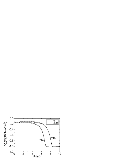
Figure 1: The Fermi average effective pairing interaction ${\cal V}^{\rm F}_{\rm eff}(R)$ for ¹²⁰Sn and ²⁰⁰Pb nuclei, at $\gamma=0$ (dashed curves) and $\gamma=0.076$ (solid curves)

In the case of proton pairing ($\tau=p$), we retain in Eq. (6) only the “strong” part of the pp potential ${\cal V}^{p}$ and then add the “bare” Coulomb potential ${\cal V}_{\rm C}$ to the BCS term of Eq. (7) ,

$${\cal V}_{p,\rm eff}^{\rm BCS}={\cal V}^{\rm BCS}_{s,\rm eff}+{\cal V}_{\rm C}.$$ (9)

Such approximation is valid because the mixed strong-Coulomb term of Eq. (6) is short-range, just as the strong term itself, but it is proportional to the small parameter of the fine structure constant $\alpha=1/137$. For matrix elements $\langle\lambda_{1}\lambda_{2}|{\cal V}_{\rm C}|\lambda_{3}\lambda_{4}\rangle$ of the bare Coulomb force this small parameter is partially compensated in the diagonal case, $\lambda_{1}=\lambda_{2}=\lambda_{3}=\lambda_{4}=\lambda$, owing to its long-range character. Such matrix elements can be estimated as $\simeq e^{2}/R$, where $R$ is the nuclear radius. For example, for $N=82$ isotonic chain it is of the order of 15-20% of the main diagonal matrix elements. It results in a$\simeq 30$% suppression of the proton gap value. So strong contribution of the Coulomb interaction to the proton pairing was reported recently in Ref. Dug2 . The above arguments to neglect the renormalization of Coulomb interaction are valid also inside the model space. In particular, the photon vertex ${\cal T}(q)$ does not change in the long-range (small $q$) limit, owing to the Ward identity. In other words, the large (long-range) Coulomb matrix elements are not changed by the strong interaction. Small (short-range) matrix elements do change, but they can be neglected. Thus, we can put $\gamma_{p}=\gamma_{n}=\gamma$ in Eq. (7) after adding the bare Coulomb interaction to the BCS term for protons.

Then, the gap equation (5) in the model space is solved in the $\lambda$-representation, with the self-consistent basis determined within the Generalized Energy Density Functional (GEDF) method Fay1 ; Fay2 ; Fay3 ; Fay4 ; Fay , where $m^{*}{=}m$ is assumed, with the functional DF3 Fay4 ; Fay . The latter is of principal importance for our approach: first, because it makes the results less model-dependent, all effects of $m^{*}\neq m$ in both model and subsidiary subspaces being attributed to the in-medium corrections beyond the pure BCS approximation, and second, because single-particle spectra of the GEDF method are, as a rule, in a better agreement with experiment than those of the popular versions of the SHF method HFB (see for comparison Ref. Tol-Sap ). The quality of the single-particle spectrum nearby the Fermi surface is very important for obtaining the correct value of the gap calculated from Eq. (2).

III Results

We solved the equations of the previous Section using the self-consistent $\lambda$-basis of the GEDF method with the DF3 functional of Refs. Fay4 ; Fay . The discretization method for the continuum states was used in the spherical box of radius $R=16\;$fm with the grid step $h=0.05\;$fm. The model space $S_{0}$ was extended up to the energy $E_{0}=40\;$MeV, the subsidiary one $S^{\prime}$, up to $E_{\rm max}=1000\;$MeV. The numerical stability of the results was checked by increasing the parameters up to $E_{0}=60\;$MeV, $E_{\rm max}=1200\;$MeV and $R=24\;$fm, and we found for the gap value a numerical accuracy of 0.01 MeV.

In this paper, we limit ourselves to semi-magic nuclei. There are several reasons for such a choice. The first one is of technical nature, namely we have only spherical code for the gap equation, and all or almost all semi-magic nuclei are spherical. The second one is that in nuclei with both non-magic subsystems there are often very “soft” low-lying $2^{+}$-states whose contributions to different quantities, in particular to the gap value, can be rather strong and non-regular. In such cases, it is difficult to expect that the simple ansatz (7) will work with an universal parameter $\gamma$. For neutron pairing, we consider the lead, tin, and calcium chains. The formulae above correspond to so-called “developed pairing” approximation AB , that amounts to impose the equality of the $\Delta^{+}$ and $\Delta^{-}$ operators and to neglect the particle-number non-conservation effects. Therefore we limit ourselves to nuclei having, as a minimum, four particles (holes) above (below) the magic core. For this reason, only the isotope ⁴⁴Ca was considered in the calcium chain.

In accordance with the recipe of Ref. milan3 , we represent the theoretical gap with the “Fermi average” combination

$$\Delta_{\rm F}=\sum_{\lambda}{(2j{+}1)\Delta_{\lambda\lambda}}/\sum_{\lambda}(2j{+}1),$$ (10)

where the summation is carried out over the states $\lambda$ in the interval of $|\varepsilon_{\lambda}{-}\mu|{<}3\;$MeV, . The “experimental” gap is determined by the usual 5-term mass difference, Eq. (13) of the Appendix. As it is argued in the Appendix, the relevance of the mass difference to the gap has an accuracy of $\simeq(0.1\div 0.2)$ MeV. Therefore, it is reasonable to try to achieve the agreement of the gap within such limits.

Let us begin from the lead chain. Results are presented in Table I. In the end of this table, the results are shown for the ⁴⁴Ca nucleus which is the lightest one among the scope “from calcium to lead” considered in this article. We try to find a value of $\gamma$ which will be universal for all the region.

Table 1: Neutron gap $\Delta^{n}_{\rm F}$ (MeV) in Pb isotopes and ⁴⁴Ca nucleus.

nucleus	$\Delta^{n}_{\rm F}$	$\Delta_{\rm exp}$

	$\gamma$=0	0.06	0.08
182Pb	1.79	1.33	1.20	1.30
184Pb	1.79	1.33	1.20	1.34
186Pb	1.78	1.32	1.19	1.30
188Pb	1.76	1.31	1.17	1.25
190Pb	1.73	1.29	1.16	1.24
192Pb	1.68	1.22	1.09	1.21
194Pb	1.62	1.16	1.03	1.13
196Pb	1.53	1.09	0.96	1.01
198Pb	1.43	1.00	0.87	0.94
200Pb	1.31	0.90	0.80	0.87
202Pb	1.16	0.79	0.69	0.78
204Pb	0.95	0.64	0.56	0.71
44Ca	1.83	1.50	1.41	1.54

In Table I the strong effect of the small phenomenological addendum in Eq. (7) is shown. The ab initio BCS result ($\gamma=0$) significantly overestimates the gap. Switching on this term with $\gamma=0.06\div 0.08$ suppresses the gap by 30 - 40%, in agreement with the data. The rms deviation of the theoretical values of the gap from the data for 13 nuclei, presented in Table I, is $\sqrt{\overline{(\delta\Delta)^{2}}}{\simeq}0.045\;$MeV at $\gamma=0.06$ and 0.103 MeV at $\gamma=0.08$. It has a minimum $\sqrt{\overline{(\delta\Delta)^{2}}}{\simeq}0.037\;$MeV at $\gamma=0.064$, but, according to the above estimate, it is not reasonable to push the accuracy too much. In any case, we may consider the parameter $\gamma\simeq 0.06$ as an optimal one for this set of nuclei.

Let us consider now the tin chain. The results are presented in Table II. Again we see a strong suppression with $\gamma=0.06\div 0.08$, but the agreement now is remarkably poorer than in the lead case. Now, the rms deviation is $\sqrt{\overline{(\delta\Delta)^{2}}}{\simeq}0.165\;$MeV at $\gamma=0.06$ and 0.169 at $\gamma=0.08$, and the minimal value $\sqrt{\overline{(\delta\Delta)^{2}}}{\simeq}0.158\;$MeV at $\gamma=0.07$ is also too large.

Table 2: Neutron gap $\Delta^{n}_{\rm F}$ (MeV) in Sn isotopes.

nucleus	$\Delta^{n}_{\rm F}$	$\Delta_{\rm exp}$

	$\gamma$=0	0.06	0.08
106Sn	1.35	0.95	0.83	1.20
108Sn	1.52	1.13	1.01	1.23
110Sn	1.65	1.26	1.14	1.30
112Sn	1.74	1.34	1.23	1.29
114Sn	1.80	1.40	1.28	1.14
116Sn	1.82	1.43	1.31	1.10
118Sn	1.83	1.44	1.32	1.25
120Sn	1.80	1.42	1.31	1.32
122Sn	1.74	1.38	1.28	1.30
124Sn	1.65	1.30	1.21	1.25
126Sn	1.51	1.19	1.10	1.20
128Sn	1.31	1.02	0.94	1.16

Let us move now to protons. The effect of the Coulomb interaction to the proton gap is shown in Table III for the isotonic chain of nuclei with the magic neutron number $N=82$. It is seen that, indeed, it is rather strong $\simeq 0.5\;$MeV, in accordance with Dug2 . Again at $\gamma{=}0.06$ the agreement is almost perfect for the most part of nuclei, and only for the two heaviest isotones the disagreement is of the order of 0.2 MeV. In this case, a possible explanation lies in that we are close to the phase transition to a deformed state (at $A\simeq 150$). Owing to the contribution of these “bad” cases, the average difference between the theoretical and experimental gaps for the $N=82$ chain is rather high, $\sqrt{\overline{(\delta\Delta)^{2}}}=0.124\;$MeV. The average error for all 34 nuclei considered is equal to $\sqrt{\overline{(\delta\Delta)^{2}}}{\simeq}0.086\;$MeV. As it follows from the analysis discussed in the Appendix, this value is within the accuracy of the experimental values of the gap extracted from the 5-term formula (13).

Table 3: Proton gap $\Delta^{p}_{\rm F}$ (MeV) for the isotone gap $N=82$.

nucleus	$\Delta^{p}_{\rm F}$	$\Delta_{\rm exp}$

${\cal V}_{\rm eff}^{p}{=}{\cal V}_{\rm eff}^{0}$

${\cal V}_{\rm eff}^{p}{=}{\cal V}_{\rm eff}^{0}+{\cal V}_{\rm C}$

		$\gamma$=0	0.06
136Xe	1.65	1.19	0.87	0.75
138Ba	1.80	1.33	0.98	0.87
140Ce	1.90	1.42	1.03	0.97
142Nd	1.99	1.48	1.06	1.00
144Sm	2.01	1.49	1.05	1.02
146Gd	2.02	1.50	1.05	1.13
148Dy	2.01	1.50	1.06	1.19
150Er	1.98	1.48	1.07	1.22
152Yb	1.92	1.44	1.05	1.29

IV The role of the single-particle spectrum

We consider the poor agreement for the tin chain as a troubling point. Indeed, this chain is a traditional benchmark for the pairing problem in nuclei, and the most strong deviation takes place for the ¹¹⁶Sn nucleus which is in the very center of the chain where the scheme used should work especially well. In searching the reasons for such a drawback, we paid attention to a new version of the DF3 functional, named DF3a Tol-Sap , in which the spin-orbit and effective tensor terms of the original DF3 functional were changed to fit new data on spin-orbit splitting in magic nuclei e_exp . The matter is that the details of neutron paring in the chain under consideration depend essentially on the position of the “intruder” state $1h_{11/2}$ which, in turn, is determined mainly by these components of the functional. We repeated the calculations for this functional DF3a and found that the agreement became much better. The optimal value $\gamma=0.052$ with $\sqrt{\overline{(\delta\Delta)^{2}}}{\simeq}0.056\;$MeV is now a little less than for the lead chain, but for $\gamma=0.06$ chosen above the agreement is also reasonably good, $\sqrt{\overline{(\delta\Delta)^{2}}}{\simeq}0.084\;$MeV. In Fig. 2 is displayed the comparison of the theoretical predictions for the pairing gap in the tin chain (both versions of the functional under consideration) with the experimental data.

Figure 2: Neutron gap in Sn isotopes

We see that, indeed, the new calculation is now in nice agreement with the data. To find the reason of so strong difference of the results for these versions of the essentially same functional, we examined the corresponding single-particle spectra along the chain comparing them with existing experimental data. Dealing with an even ^ASn isotope, there is a dilemma how to consider a state $|i\rangle$ under consideration, either the hole state (i.e. the excitation of the ^A-1Sn nucleus) or the particle one (the excitation of the ^A+1Sn nucleus). We use a simple recipe: the state $|i\rangle$ is considered as a hole state if the inequality $v_{i}^{2}>0.5$ takes place and as a particle state otherwise. Note that in the case of $v_{i}^{2}\simeq 0.5$ the difference between the particle and hole energies is, as a rule, quite small. In general, both the functionals reproduce the experimental low-lying levels sufficiently well. In particular, the spin of the ground state of odd isotopes is always reproduced correctly for both calculations. But there is a noticeable difference for the $1h_{11/2}$ state in the left part of the chain, till ¹²²Sn, see Fig. 3.

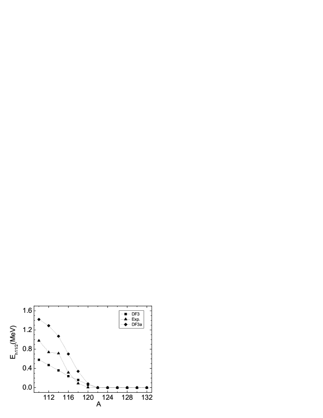
Figure 3: The $h_{11/2}$ level position accounted from the ground state in Sn isotopes

In this region, its position is systematically lower than the experimental one for the DF3 functional and systematically higher, for the DF3a functional. In the vicinity of the ¹¹⁶Sn nucleus, this difference becomes dramatic and the too low position of the $1h_{11/2}$ state in the DF3 case leads to an incorrect enhancement of the gap value.

In Fig. 4, the single-particle spectrum of the ¹¹⁴ Sn nucleus calculated for the two versions of the functional is compared with the experimental one. Each theoretical level is supplemented with the $(2j_{i}+1)u_{i}v_{i}$ factor that determines mainly the contribution of the $i$-level to the gap equation. The same for ¹¹⁶Sn nucleus is displayed in Fig. 5. We see that for all other states $|i\rangle$ these factors are rather close for the two versions of the functional, but for the $1h_{11/2}$ state the difference is rather strong. As to heavy tin isotopes for which this level becomes the ground state for both functionals, the difference between their predictions for the gap value are quite close, see Fig. 2.

Figure 4: ¹¹⁴Sn spectrum

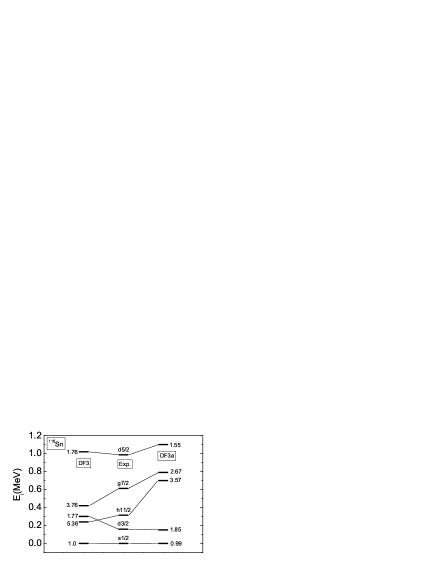
Figure 5: ¹¹⁶Sn spectrum

This analysis shows the great sensitivity of the gap value to the single-particle spectrum nearby the Fermi level, especially to the position of levels with high $j$-value. Therefore it is interesting to examine which effect is to be expected in the other cases of going from the initial DF3 functional to this new version. It is displayed in Fig. 6 for the lead isotopes. We see that in this case the overall agreement for the new version of the functional becomes worse. Evidently, again the position of high $j$-levels is different, in favor of the DF3 functional in this case.

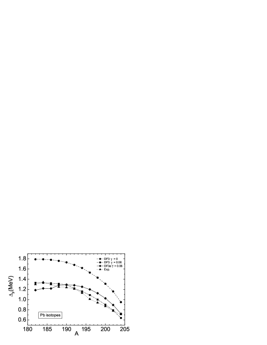
Figure 6: Neutron gap in Pb isotopes.

A bad situation for the DF3a functional rises for the $N=82$ isotone chain, see Fig. 7. The analysis shows that again the $1h_{11/2}$ level is guilty, now for protons. For the DF3a functional it is again higher than the experimental position, and for ¹⁴⁴Sm and ¹⁴⁶Gd nuclei much higher. As the result, it does not practically contribute to the gap equation resulting in a too small gap value.

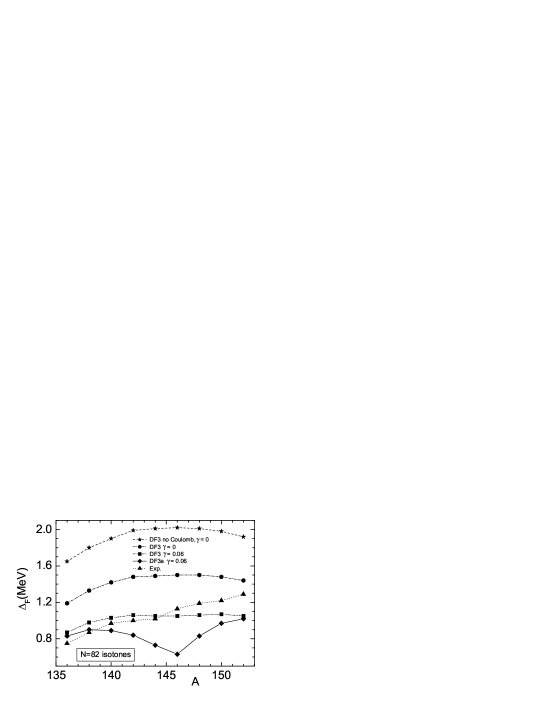
Figure 7: Proton gap for $N=82$ isotones

V Conclusion

We suggest a simple semi-microscopic model for the nuclear pairing starting from the ab initio BCS gap equation. The self-consistent GEDF Method basis, characterized by the bare nucleon mass, is employed in the calculation. The gap equation is recast in the model space $S_{0}$, replacing the bare interaction with the effective pairing interaction determined in the complementary subspace $S^{\prime}$.

The Argonne v₁₈ potential was adopted along with the LPA method. A small phenomenological term is added to this effective interaction that contains one parameter which should embody approximately the effective mass and various corrections to the pure BCS theory. Calculations are carried out with the DF3 functional Fay4 ; Fay for semi-magic lead and tin isotopic chains and the $N=82$ isotonic chain as well. The Coulomb interaction is explicitly included in the proton gap equation. We find that the model reproduces rather well the experimental values of the neutron and proton gaps in semi-magic nuclei. The overall agreement ($\sqrt{\overline{(\delta\Delta)^{2}}}{\simeq}0.13\;$MeV) is better than that obtained in Ref. Dug1 , where the authors did not introduce free parameters explicitly but they made it implicitly by using a specific $k$-dependence in the effective mass.

We examine also the role of the single-particle spectrum in the gap equation. For this aim we use the new modification DF3a Tol-Sap of the functional Fay4 ; Fay that changes spin-orbit and effective tensor terms. The use of this functional gives an agreement better for the tin chain and worse for the lead chain and even more for the $N=82$ chain. The accuracy of the predictions depends strongly on the quality of reproducing the positions of high $j$-levels in the self-consistent basis used. We are thinking, e.g., to the $1h_{11/2}$ neutron level in the tin isotopes and $1h_{11/2}$ proton level for $N=82$ isotones.

The ansatz of Eq. (7) exhibits an obvious drawback. The phenomenological GEDF pairing interaction of Ref. Fay contains the surface term (${\propto}(d\rho/dr)^{2}$) that plays an essential role for the description of the odd-even effect (staggering) in nuclear radii. It originates mainly from the exchange by surface phonons which was explicitly taken into account in milan2 ; milan3 . The addition, to such a term in Eq. (7) is associated the introduction of a new parameter, and at the first stage we prefer to avoid that. A more consistent scheme should, evidently, include the explicit consideration of the low-lying phonons, as e.g. in milan2 , but taking into account the so-called tadpole diagrams Kam_S . In this case, the phenomenological constant $\gamma$ should, of course, change.

Acknowledgments

We thank G. L. Colo, T. Duguet, V. A. Khodel and S. V. Tolokonnikov for valuable discussions. This research was partially supported by the joint Grants of RFBR and DFG, Germany, No. 09-02-91352-NNIO_ , 436 RUS 113/994/0-1(R), by the Grants NSh-7235.2010.2 and 2.1.1/4540 of the Russian Ministry for Science and Education, and by the RFBR grants 09-02-01284-a, 09-02-12168-ofi_m. Two of us (S. P. and E. S.) thank the INFN, Sezione di Catania, for hospitality.

Appendix A Accuracy of extracting experimental gap values from the mass differences

In this Appendix, we discuss the accuracy of determination of the “experimental” gap, $\Delta_{\rm exp}$, from the mass data. Usually, this quantity is found in terms of mass values $M$ of neighboring nuclei via 3-term formulae,

$$2\Delta^{+}_{\rm exp}(A)=\delta_{2}M^{+}\equiv 2M(A+1)-M(A+2)-M(A)$$ (11)

or

$$2\Delta^{-}_{\rm exp}(A)=\delta_{2}M^{-}\equiv 2M(A-1)-M(A-2)-M(A).$$ (12)

The 5-term expression is usually considered more accurate, being a half-sum of them,

$$\Delta_{\rm exp}(A)=\overline{\delta_{2}M}/2\equiv(\delta_{2}M^{+}+\delta_{2}M^{-})/4.$$ (13)

These simple recipes were used, in particular, in milan2 ; milan3 ; Dug1 ; Dug2 . However, they originate from the simplest model of $\Delta={\rm const}$, and the accuracy of such prescription is not a priori obvious. To clarify this point we made a calculation which could be considered as a “theoretical experiment”. We used the GEDF method Fay with the functional DF3 which reproduces the mass differences of Eqs. (11), (12) type sufficiently well. We calculated first directly the right side of Eq. (13) and second, the theoretical gap value with Eq. (10) within the same GEDF method. The comparison of these two quantities is given in Fig. 7 for the lead isotopes and in Fig. 8 for the tin isotopes. We see that for the main part of nuclei under consideration the difference between values in two neighboring columns is within 0.1 MeV. However, there is several cases where it is of the order (or even exceeds) 0.2 MeV. Leaving aside detailed analysis of these “bad” cases we are forced to put a limit of $\simeq 0.1-0.2\;$MeV for the accuracy of the experimental gap determined from Eq. (13).

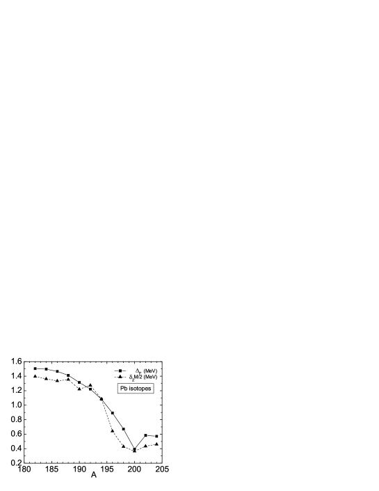
Figure 8: The theoretical predictions for the mass difference $\overline{\delta_{2}M}/2$ (triangles) versus the average gap value $\Delta_{\rm F}$ (squares) for Pb isotopes. Both the quantities are calculated within the GEDF method, see the text.

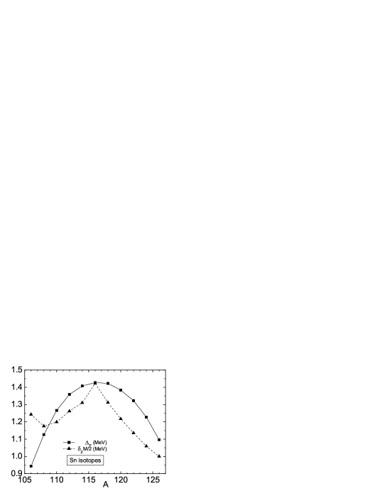
Figure 9: The same as in Fig. 1, but for Sn isotopes.

References

- (1) F. Barranco, R. A. Broglia, H. Esbensen, and E. Vigezzi, Phys. Lett. B390, 13 (1997).
- (2) F. Barranco, R. A. Broglia, G. Colo, et al., Eur. Phys. J. A 21, 57 (2004).
- (3) A. Pastore, F. Barranco, R. A. Broglia, and E. Vigezzi, Phys. Rev. C 78, 024315 (2008).
- (4) T. Duguet and T. Lesinski, Eur. Phys. J. Special Topics 156, 207 (2008).
- (5) K. Hebeler, T. Duguet, T. Lesinski, and A. Schwenk, Phys. Rev. C 80, 044321 (2009).
- (6) E. Chabanat, P. Bonche, P. Haensel, J. Meyer, and R. Schaeffer, Nucl. Phys. A627, 710 (1997).
- (7) M. Baldo, U. Lombardo, S.S. Pankratov, E.E. Saperstein. J. Phys. G: Nucl. Phys., 37, 064016 (2010).
- (8) U. Lombardo, P. Schuck, and W. Zuo, Phys. Rev. C 64, 021301(R) (2001).
- (9) L. G. Cao, U. Lombardo, P. Schuck, and W. Zuo, Phys. Rev. C 74, 064301 (2006).
- (10) S. Gandolfi , A.Y. Illarionov, F. Pederiva, K. E. Schmidt, and S. Fantoni , Phys. Rev. C 80, 045802 (2009).
- (11) S. K. Bogner, T. T. S. Kuo, and A. Schwenk, Phys. Rep. 386, 1 (2003).
- (12) S. S. Pankratov, M. Baldo, M. V. Zverev, U. Lombardo, E. E. Saperstein, S. V. Tolokonnikov, JETP Lett., 90, 612 (2009).
- (13) S. S. Pankratov, M. Baldo, M. V. Zverev, U. Lombardo, E. E. Saperstein, JETP Lett., 92, 92 (2010).
- (14) A. B. Migdal Theory of finite Fermi systems and applications to atomic nuclei (Wiley, New York, 1967).
- (15) M. Baldo, U. Lombardo, E. E. Saperstein, M. V. Zverev, Nucl. Phys. A628, 503 (1998).
- (16) M. Baldo, U. Lombardo, E. E. Saperstein, and M. V. Zverev Phys. Rep. 391, 261 (2004).
- (17) E. E. Saperstein, S. S. Pankratov, M. V. Zverev, M. Baldo, U. Lombardo, Phys. At. Nucl., 72, 1059 (2009).
- (18) M. Baldo, O. Elgaroy, L. Engvik, M. Hjorth-Jensen, and H.-J. Schulze, Phys. Rev. 58, 1921 (1998).
- (19) L.-W. Siu, J. W. Holt, T. T. S. Kuo, and G. E. Brown, Phys. Rev. C 79, 054004 (2009).
- (20) M. Baldo and A. Grasso, Phys. Lett. B485, 115 (2000).
- (21) M. Baldo and A. Grasso, Phys. At. Nucl. 64, 611 (2001).
- (22) V. N. Borzov, E. E. Saperstein, S. V. Tolokonnikov, Phys. At. Nucl. 71, 493 (2008).
- (23) W. Zuo, C. W. Shen and U. Lombardo, Phys. Rev. C 67, 037301 (2003).
- (24) A. V. Smirnov, S. V. Tolokonnikov, S. A. Fayans, Sov. J. Nucl. Phys. 48, 995 (1988).
- (25) S. A. Fayans, E. L. Trykov, and D. Zawischa, Nucl. Phys. A568, 523 (1994).
- (26) D. J. Horen, G. R. Satchker, S. A. Fayans, and E. L. Trykov, Nucl. Phys. A600, 1993 (1996).
- (27) S. A. Fayans, JETP Lett. 68, 169 (1998).
- (28) S. A. Fayans, S. V. Tolokonnikov, E. L. Trykov, and D. Zawischa, Nucl. Phys. A676, 49 (2000).
- (29) S. Goriely, N. Chamel, and J. M. Pearson, Phys. Rev. Lett. 102, 152503 (2009).
- (30) S. V. Tolokonnikov and E. E. Saperstein, Phys. At. Nucl. 73, 1684 (2010).
- (31) H. Grawe, report on Workshop on “Nuclear Structure in 78Ni region”, Leuven, 2009, March 9-11
- (32) S. S. Pankratov, M. Baldo, U. Lombardo, E. E. Saperstein, and M. V. Zverev, Phys. At. Nucl., 70, 688 (2007).
- (33) S. Kamerdzhiev and E. E. Saperstein, Eur. Phys. J. A 37, 333 (2008).