Shining Light on Merging Galaxies I:
The Ongoing Merger of a Quasar with a ‘Green Valley’ Galaxy

Abstract

Serendipitous observations of a pair $z=0.37$ interacting galaxies (one hosting a quasar) show a massive gaseous bridge of material connecting the two objects. This bridge is photoionized by the quasar (QSO) revealing gas along the entire projected 38 $h_{72}^{-1}\,\rm kpc$ sightline connecting the two galaxies. The emission lines that result give an unprecedented opportunity to study the merger process at this redshift. We determine the kinematics, ionization parameter ($\log U\approx-2.5\pm 0.03$), column density ($N_{H,\perp}\approx 10^{21}\mbox{ cm}^{-2}$), metallicity ([M/H]$\approx-0.20\pm 0.15$), and mass ($\approx 10^{8}M_{\odot}$) of the gaseous bridge. We simultaneously constrain properties of the QSO-host ($M_{DM}>8.8\times 10^{11}$) and its companion galaxy ($M_{DM}>2.1\times 10^{11}$; $M_{\star}\sim 2\times 10^{10}M_{\odot}$; stellar burst age=$300-800$ Myr; SFR$\sim 6\ M_{\odot}$ yr^-1; and metallicity $12+\log$(O/H)=$8.64\pm 0.2$). The general properties of this system match the standard paradigm of a galaxy-galaxy merger caught between first and second passage while one of the galaxies hosts an active quasar. The companion galaxy lies in the so-called ‘green valley’, with a stellar population consistent with a recent starburst triggered during the first passage of the merger and has no detectable AGN activity. In addition to providing case-studies of quasars associated with galaxy mergers, quasar/galaxy pairs with QSO-photoionized tidal bridges such as this one offer unique insights into the galaxy properties while also distinguishing an important and inadequately understood phase of galaxy evolution.

1. Introduction

The paradigm of hierarchical structure formation is based on the frequent mergers of galaxies and their dark matter halos, as predicted and quantified by cosmological simulations which construct merger trees to track the merger history of halos (e.g. Springel et al., 2005b; Fakhouri et al., 2010). Observations of galaxies ‘caught in the act’ of merging (e.g. Arp, 1966; Lotz et al., 2008b) support this theory. Galaxy mergers are believed to be an important phase of galaxy evolution and are thought to be crucial to understanding super-massive black hole (SMBH) growth, galaxy morphologies, and the truncation of star-formation within galaxies.

While details of the merger process depend on the orbit, mass ratio and morphologies of the galaxies involved, the basic sequence of events for a major (galaxy mass ratio $\gtrapprox$  1:4) is relatively well agreed upon (Mihos & Hernquist, 1994, 1996; Hopkins et al., 2008a; Cox et al., 2006; Di Matteo et al., 2007; Chilingarian et al., 2010). Galaxies undergoing a merger typically have orbital angular momentum that prevents direct collisions and leads to a series of close passages which have progressively smaller apogees due to dissipation in the merger. During their first close passage, the galaxies exert strong tidal forces on each other. For galaxies with a small bulge component, these tidal forces lead to bar formation. The stellar bar lags behind the gaseous bar inducing a torque on the gas which leads to the funneling of gas towards the center of the galaxy. The inflow also leads to higher central gas surface densities which is predicted to spur enhanced star formation (e.g. Mihos & Hernquist, 1996).

Subsequent close passages lead to smaller inflows as a large fraction of the available gas was used up during a first-passage ‘starburst’. The second major phase of inflow, therefore, occurs later due to a different mechanism as the galaxies are engaged in final coalescence. At that time, the remaining gas is brought rapidly to the center by dissipation into a dense compact central structure that rapidly forms stars. The final remnant galaxy in merger simulations is commonly an elliptical, dispersion-dominated system that has ceased star-formation because its gas reservoir is used up in the starbursts and lost via stellar or AGN feedback (e.g. Springel et al., 2005a). However, the details of the effectiveness of ‘quenching’ star-formation and the actual process that is responsible varies between different studies and depends on the choice of numerical prescription.

For galaxies with large bulge components, the initial bar formation is suppressed and star formation is far less elevated in the early stages of the merger. Consequently, there is a large reservoir of gas remaining until the stages of final coalescence and the final starburst is more extreme. Because the galaxies coalesce over a short timescale, the final starburst can be more intense than that of a bulgeless galaxy during first passage.

Some studies (Hopkins et al., 2008a; Springel et al., 2005a) argue that these merger events lead to elevated levels of AGN activity and ultimately a quasar (QSO) phase which is short ($10^{6}-10^{8.5}$ yrs; Martini & Weinberg, 2001; Martini & Schneider, 2003) and extremely bright ($\sim 10^{46}\,\mbox{erg/s}$). This phase of the supermassive black hole (SMBH) evolution is thought to dominate the mass accretion history of the black hole (Soltan, 1982) and can profoundly affect its host. During final coalescence, the large gas densities near the center of the galaxy (where the SMBH is located) leads to a large amount of efficient AGN fueling that manifests as a QSO phase. This scenario is supported by observations of quasar hosts showing disturbed morphologies (e.g. Bennert et al., 2008; Green et al., 2010) consistent with being merger remnants. Observations disagree on whether mergers lead to elevated levels of AGN activity in the early stages of the merger (i.e. between first and second passage) with some (e.g., Woods & Geller, 2007) suggesting an increase and others (e.g., Ellisonet al., 2008) suggesting no increase in activity at these early stages.

In addition to their obvious role in increasing galaxy mass, mergers provide a tantalizing solution to several observed cosmological trends. Firstly, they offer a convenient explanation for the various SMBH-host relations. Naïvely, the SMBH (which only has a gravitational sphere of influence $\approx 1/1000$ the size of the host) should have no correlation with the properties of its host. However, SMBHs have been observed to be correlated with their host’s stellar mass (Magorrian et al., 1998), velocity dispersion (Gebhardt et al., 2000; Ferrarese & Merritt, 2000), dark matter halo mass (Ferrarese, 2002), and morphology (Graham et al., 2001). If black holes are growing in galaxy mergers at the same time that many of these other galactic properties are changing, then this may explain the observed correlations with the host. In fact, it has been proposed that this simultaneous evolution can lead to these various correlations even without invoking any AGN feedback (Sutter & Ricker, 2010).

Mergers may also be a key ingredient in quenching star-formation within galaxies. The basic picture is that galaxies can be broadly classified into one of two groups: (1) actively star forming spiral “blue cloud” galaxies or (2) passively evolving elliptical “dead” red sequence galaxies. It appears that the red-sequence galaxies somehow evolve from actively star-forming galaxies (see Faber et al., 2007). These hypotheses raise the question of how actively star-forming galaxies are “terminated” to produce red-sequence galaxies. While there have been many theories proposed (e.g., halo quenching; Dekel & Birnboim, 2006), one of the more popular solutions is through the AGN activity, starbursts, and feedback induced by galaxy mergers (e.g. Hopkins et al., 2008a). In such a paradigm, the sequence of events (as described above) of the merger lead to a burst of star formation and AGN activity whose feedback can unbind a large fraction of the remaining gas. This quenches the galaxy while the merger also leaves the remnant with an elliptical morphology, seemingly consistent with observations (Toomre, 1977).

This theory is not without its flaws. Observational evidence suggests that galaxies transitioning from the “blue cloud” to red sequence (i.e. “green valley” galaxies) do not appear to be dominated by merger remnants (Reichard et al., 2009) nor the result of rapid quenching (Martin et al., 2007). Nevertheless, it has established a theoretical framework that, in principle, can be tested with empirical observation.

The details of SMBH fueling and feedback as well as star formation and supernova feedback are crucial to understanding the actual role that mergers play in galaxy evolution. However, merger simulations cannot realistically implement these processes due to the relevant physical scales spanning a dynamic range of sub-pc to many kpc scales. Additionally, simulations are regularly unable to accurately couple radiative transfer to the hydrodynamics due to high computational expense. Simulators are thus forced to implement tuned sub-grid models which sometimes are not physically well-motivated (e.g., using Bondi-Hoyle accretion; see Booth & Schaye (2009)). Thus there remain many open questions about the processes at work during a galaxy merger that simulations will be unable to enlighten for the foreseeable future. As such, observations are required to improve our understanding and guide future theoretical effort. However, observational studies of these processes are challenging for a number of reasons. In contrast to studies of nearby, merging galaxies which permit sensitive searches for disturbed morphologies and faint tidal structures (e.g., Arp, 1966), such analysis at higher redshift becomes prohibitive owing to the great distance. Low surface brightness tidal features are too faint to observe and one requires much higher angular resolution to detect small morphological features at higher redshift. Additionally, for all but the nearest galaxies (e.g., Hibbard et al., 2001), observational studies of mergers are limited to studying the stellar distribution because the emission from the bulk of the gas is invisible at cosmological distances. However, it has been shown that gas and stars may have completely different velocity structures and distributions, especially in systems where a galaxy is undergoing a phase of enhanced AGN activity (Greene et al., 2009). Since the dynamics of the gas and not the stars ultimately fuel AGN activity and star formation, meaningful studies of these processes require the ability to study gas in mergers. Lastly, while the various feedback prescriptions may be tuned to match global properties of an ensemble population of galaxies, they must also be tested against actual merging systems.

This gap in our understanding motivated a novel method for finding and studying merging galaxies that is inspired by the serendipitous discovery of a remarkable prototype. In our method, we search for systems where the ionizing flux of the quasar “lights up” the gas in a merger in order to find new observational constraints on merger models.

With an ionizing photon flux ($S$) of $\approx 10^{56}$ photons/s/sr (Tadhunter, 1996), a quasar can ionize gas to conditions comparable to H II regions out to distances of 60 kpc. While observations of highly ionized gas with large (tens of kpc) spatial extent known as extended emission line regions (EELRs) have been known for decades (Matthews & Sandage, 1963; Wampler et al., 1975; Stockton & MacKenty, 1987; Penston et al., 1990; Fu & Stockton, 2009), our study focuses on a novel application of this standard result where we utilize quasar photoionization to study a pair of merging galaxies. In detail, we focus on an EELR produced by a quasar that has been triggered by a merger event. During such a merger, one also expects extended tidal features of gas out to distances of  100 kpc that may be photoionized by the quasar and could thus be rendered visible through recombination and forbidden lines. Observations have confirmed that such extended material that may be associated with a galaxy merger can be seen in emission lines near at least one quasar (Villar-Martín et al., 2010).

Our prototype was serendipitously discovered while selecting targets for a study of gas in the extended halos of galaxies via quasar sight lines (Tumlinson et al in prep.). That study used the Sloan Digital Sky Survey DR5 (Adelman-McCarthy et al., 2007) to find foreground galaxies close to quasar sight lines based on photometric redshifts. However the galaxy they had hoped to be in front of J2049-0012 (a z=0.369 quasar) by a cosmological distance was in fact found to have the same redshift. Further inspection revealed that the long-slit spectrum of the system contained bright emission lines along a remarkable gas “bridge” connecting the quasar to its companion galaxy, 38 $h_{72}^{-1}\,\rm kpc$ away in projection, and photoionized by the hard spectrum of the quasar. This bridge is most likely the result of a tidal interaction of the galaxies during the first passage of their ongoing merger. The extended gas around these objects, normally completely invisible at this distance, is being lit-up by radiation from the quasar. This provides an unparalleled opportunity to study the kinematics and structure of the gas in the merger, which otherwise we would not have even known was occuring. At the same time, we have detailed measurements of the galaxy properties, including the outer regions of the quasar’s host galaxy. The companion galaxy is also a member of the ‘green valley’ and we are afforded the chance to examine this poorly understood and rare phase of galaxy evolution in this merger context.

This is the first in a pair of papers on this particular system. This paper focuses on the details of the merging system (mass ratio, timescales, separation, merger stage, companion galaxy properties, SMBH mass and luminosity) as well as discussion of the emission line bridge and an explanation for its ionization source. Paper II focuses on the quasar including its lifetime, isotropy, impact on companion galaxy, implications for its triggering, and the placement of the SMBH on Magorrian-like relations at a peculiar phase of its evolution.

We assume a cosmology with $\Omega_{\Lambda}=0.73$, $\Omega_{M}=0.27$, and $H_{0}=72\ h_{72}\rm km\,s^{-1}\,Mpc^{-1}$.

The paper is organized as follows: $\S$ 2 describes the observations of this system; $\S$ 3 gives an overview of the results of the observations; $\S$ 4 details our measurements of emission line fluxes and kinematics; $\S$ 5 describes the inferred properties of the interacting pair of galaxies; $\S$ 6 discusses our analysis of the bridge connecting the galaxies including our analysis of its origin; $\S$ 7 presents further discussion; $\S$ 8 presents a summary.

Table 1Observations

Instrument	Slit	Dichroic	Camera	Disperser	Resolution [km/s]	Filter	Exposure	Standard Star	Date
	[′′]					[s]		(UT)
Keck/LRIS	1.0	D560	R	600/7500 (28.15)	160	$\cdots$	900x2	Feige 110	2008-10-03
Keck/LRIS	1.0	D560	B	600/4000	240	$\cdots$	830x2	Feige 110	2008-10-03
Keck/LRIS	1.0	D560	R	600/7500 (29.15)	160	$\cdots$	300x3	BD+28	2009-09-17
Keck/LRIS	0.7	D560	R	1200/7500 (40.15)	65	$\cdots$	600x2	BD+28	2009-09-17
Shane/Kast	1.0	d55	R	600/7500 (10775.6)	$\cdots$	$\cdots$	1800	$\cdots$	2009-05-26
Keck/LRIS	$\cdots$	D560	B	$\cdots$	$\cdots$	B	60,200,230x2	$\cdots$	2008-10-03
Keck/LRIS	$\cdots$	D560	R	$\cdots$	$\cdots$	R	90,200x3	$\cdots$	2008-10-03

2. Observations & Data Reduction

We obtained a set of spectroscopic and imaging observations of this quasar/galaxy pair using the dual-channel Low Resolution Imaging Spectrometer (LRIS; Oke et al., 1995) on the Keck I 10m telescope and the dual-channel Kast spectrometer (Miller & Stone, 1993) on the 3m Shane telescope at Lick Observatory (see Table 1).

Two long slit spectra were taken using LRIS with a 1.0^′′ slit width, D560 dichroic, 600/4000 grism, and 600/7500 grating tilted to an angle of 28.15^∘. This gave a red wavelength coverage of roughly 5600 to 8200Å, a dispersion of 0.63 Å/pixel, and FWHM $\approx 160\ {\rm km~{}s^{-1}}$. In the blue we had coverage of 3100 to 5600 Å  with FWHM $\approx 240\ {\rm km~{}s^{-1}}$. Subsequently we took further LRIS observations with the grating angle tilted to 29.15 giving us coverage of 6300-9500 Å to cover H$\alpha$ and [N II] emission of our z=0.37 system. We also took a higher resolution spectrum covering the [O III] emission lines to better characterize the gas kinematics. We used the 0.7^′′ long slit, D560 dichroic, and 1200/7500 grating blazed to an angle of 40.15. This gave a dispersion of 0.4 Å/pix^-1, FWHM$~{}\approx 65\ {\rm km~{}s^{-1}}$, and wavelength coverage of roughly $6100-7000$Å. The FWHM for each of these setups was estimated by measuring the parameters of Gaussian models fit to sky lines in the science exposures.

All of the above spectra were taken with the long slit aligned along the line connecting the two sources (so that both the quasar and companion galaxy were within the slit). Another spectrum was taken using the Lick Observatory’s Shane 3-meter with the Kast spectrograph. This spectrum was taken with a position angle (PA) perpendicular to the line connecting the quasar/galaxy pair, roughly halfway in between (such that neither the quasar nor the companion were in the slit). This spectrum was taken with the d55 dichroic and 600/7500 grating. This grating was tilted to span a wavelength range of approximately $5500-8300$Å  with a dispersion of 2.37 Å/pixel.

Additionally we imaged the system with the LRIS camera for one 60, one 200, and two 230 second exposures in the $B$ band as well as one 90, and three 200 second exposures in the $R$ band (2008-10-03). The seeing was $\approx 0.64^{\prime\prime}$ FHWM.

We reduced the spectra using the Low-Redux pipeline developed by J. Hennawi, S. Burles, D. Schlegel, and J. X. Prochaska. We implemented this program to perform the following procedures: (1) process the flats, (2) use arcs to make a 2-dimensional wavelength image, (3) make a slit profile, (4) process the images, (5) identify objects in the slit and trace them, (6) perform sky subtraction, (7) extract the spectra, (8) correct for flexure of the spectrograph using sky lines, and (9) create a sensitivity function from a standard star. Slight modifications to the standard pipeline were necessary to perform sky subtraction due to the extended emission and the proximity of the galaxy to the quasar. Specifically, we turned off local sky subtraction after verifying that a global fit provided a good estimate of the sky background in the region of interest. Next, we coadded the images using Long-Coadd2d, a code developed by Robert da Silva and Michele Fumagalli, removing cosmic rays through comparisons of the separate exposures.

The atmosphere and instrument response influence the intensity and shape of the recorded spectrum. For point sources, the standard procedure to convert the observed spectrum into astronomical flux units is to construct a sensitivity function from the spectrum of a spectrophotometric standard star observed with the same instrumental configuration. This is done in 1-dimension, meaning that a 1-dimensional spectrum is extracted from the 2D output spectrum from the instrument and is then compared with a 1D model. We performed this procedure and applied the resulting sensitivity function to the objects extracted in the slit.

Unfortunately the region near the dichroic ($\lambda\approx 5400-5600$Å) was particularly difficult to calibrate for the 2008-10-03 observations. In particular, we find that the fluxing resulted in a galaxy spectrum that had an unphysical behavior near the dichroic. We correct for this through comparison of our Keck/LRIS spectrum of the QSO and the SDSS spectrum of the same QSO. Although the absolute and relative fluxes of quasars are known to vary, the color variation is generally small for rest wavelengths greater than 2500 Å (Wilhite et al., 2005). Avoiding issues that may arise from Fe emission lines we only sought to fit the general shape of the continuum across the boundary. In order to account for any discrepancies between ours and the SDSS fluxing, we matched the spectra by allowing our Keck/LRIS spectrum to be multiplied by a polynomial in wavelength. To find the best such 2nd order polynomial we used the singular valued decomposition method. Once the overall shapes of the spectra was matched using the above procedure, we fit a 3rd degree polynomial to each side of the dichroic for both the SDSS and matched LRIS 2008-10-03 spectra. The ratio of those polynomial fits was used to correct the LRIS spectra. Thus the spectrum correction forces the LRIS spectrum of the QSO to have the same shape in the region around the dichroic as the SDSS spectrum. This same correction was then applied to the companion galaxy spectrum.

The final product from the above procedure was a sensitivity function that converts electrons per second per spectral pixel into astronomical flux units. This allows us to calibrate the extracted, 1D spectrum of any object in the slit. Our data, however, features extended emission that spans many arcseconds spatially. Therefore we also require a 2-dimensional flux calibration that converts electrons per second per detector pixel into surface brightness units. To accomplish this task, we needed to apply the 1-dimensional fluxing (which has a mapping of pixel to sensitivity that is accurate at the center of the slit), to the entire 2D spectrum. Assuming that the appropriate correction factor is only a function of wavelength (specifically that there was a 1-to-1 mapping of wavelength to sensitivity) we can apply this correction to the entire CCD using the 2-dimensional wavelength image constructed with Low-Redux from the arc-lamp images. Interpolation of our sensitivity function evaluated at every pixel’s wavelength gives a correction factor which we then apply to the spectra.

Since we had taken long slit data, each of our spectra had portions of the CCD illuminated only by the sky. We used these to test the 1-to-1 assumption described above by measuring sigma-clipped medians along the spectral direction across spatial regions. The spatial variation in sensitivity along the slit was found to be at most a 1% effect.

3. J2049-0012: Observational Characteristics

This section provides a qualitative overview of the properties of the J2049-0012 system. More quantitative analysis is presented in the sections that follow.

Table 2Compiled Photometric Measurements

	Quasar	Galaxy	Extinction	Ref
	(mag)	(mag)	(mag)
$FUV$	$18.54\pm 0.108$	$\cdots$	0.46
$NUV$	$18.44\pm 0.063$	$\cdots$	0.49
$u$	$18.05\pm 0.01$	$21.42\pm 0.28$	0.46
$g$	$17.89\pm 0.01$	$20.93\pm 0.05$	0.34
$r$	$17.79\pm 0.01$	$19.87\pm 0.03$	0.25
$i$	$17.75\pm 0.01$	$19.62\pm 0.04$	0.19
$z$	$17.10\pm 0.01$	$19.46\pm 0.11$	0.13
$J$	$16.51\pm 0.142$	$\cdots$	$0.08$
$H$	$15.74\pm 0.150$	$\cdots$	$0.05$
$K$	$14.62\pm 0.101$	$\cdots$	$0.03$

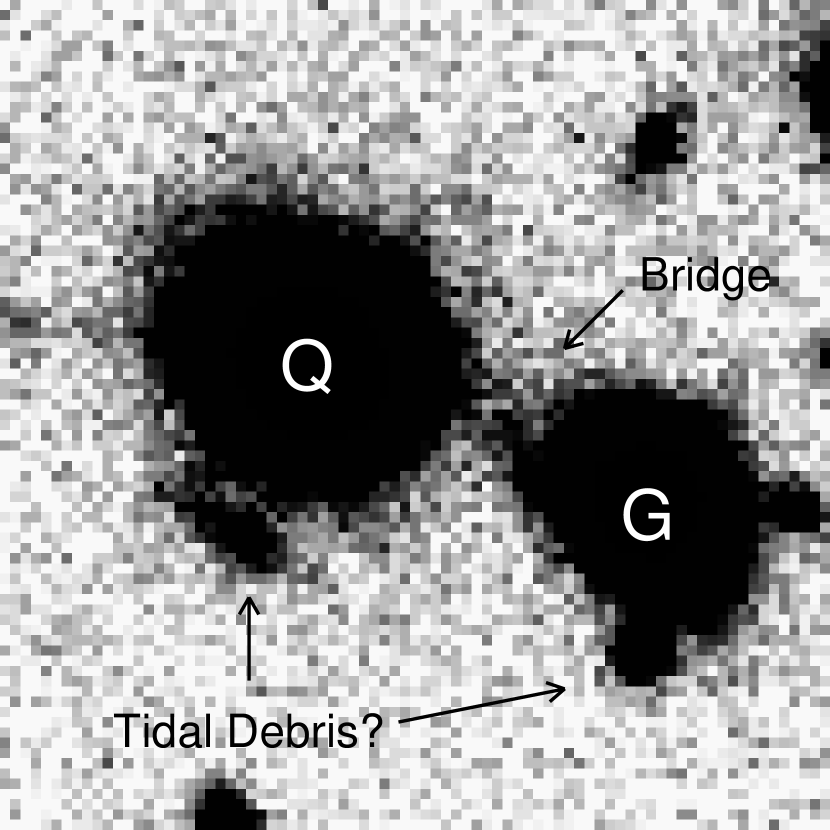
Figure 1.— R-band image (which covers the redshifted [O III] and H$\beta$ lines) zoomed in on the position of the galaxy/quasar pair. The image is 17^′′ on a side and is oriented so that N is up and E is left. One can discern the bridge connecting the two galaxies as well as some possible tidal debris. The quasar (Q) and companion galaxy (G) are separated by 8^′′, corresponding to $38h_{72}^{-1}$ kpc at $z=0.3693$.

3.1. Imaging

This quasar/galaxy pair was selected from the SDSS Data Release 5 (Adelman-McCarthy et al., 2007) and GALEX DR3 (Martin et al., 2005) catalogs as a candidate system for an HST/COS survey designed to study the gas surrounding $z\sim 0.2$ galaxies with absorption-line spectra of UV bright, background quasars (Cycle 17, ID=11598; PI: Tumlinson). The quasar photometry and redshift ($z_{\rm q}=0.3693$) were known from SDSS observations while the galaxy’s SDSS photometry yields a photometric redshift $z_{\rm phot}=0.28\pm 0.09$ (Oyaizu et al., 2008), suggesting it lay foreground to the quasar. Fig. 1 presents the R band imaging from Keck/LRIS. The quasar (J2049$-$0012) is the bright point source at the center of the image and the galaxy (J204956.61$-$001201.7) is offset by 8^′′ (38 $h_{72}^{-1}$ projected kpc) to the SW (lower right).

The companion galaxy as seen in an SDSS finding chart is a peculiar green, uncommon for galaxies observed in the SDSS. This is illustrated in Fig. 2 which compares the restframe color and absolute magnitude of this galaxy to a sample of DEEP2 galaxies at $0.3<z<0.4$ (Davis et al., 2003, 2007; Coil et al., 2004; Willmer et al., 2006). We find that the color of J204956.61$-$001201.7 places it between the two primary populations of red and blue galaxies. Such galaxies are commonly described as lying within the ‘green valley’, a region that possibly marks the transition from blue star-forming galaxies to red, quiescent systems (Faber et al., 2007). The processes that drive galaxies into the green valley are not well established. Scenarios include merger-induced star bursts where the tidal forces the galaxies exert on each other funnel gas towards their centers (Quintero et al., 2004), which in turn fuels a massive starburst and ultimately a bright quasar phase (Hopkins et al., 2008b). Such a model predicts that the green valley region should coincide with AGN activity, which is supported by recent observational evidence (e.g. Schawinski et al., 2009; Nandra et al., 2007). However, the level of AGN activity in the companion galaxy in our quasar/galaxy pair is unclear. The 1d extraction of our galaxy shows faint [Ne V]$\lambda\lambda 3426,3346$ emission (a commonly used indicator of AGN activity), but even this emission may be the result of photoionization by the neighboring quasar.

Additionally, such a model may also predict that objects in the ‘green valley’ have transitional stellar populations such as those of post-starburst galaxies. This is supported by observational studies (e.g., Vergani et al., 2010; Kocevski et al., 2009). These galaxies have their light dominated by a stellar population that has aged past the point where its stellar light is dominated by O and B stars. Examination of our spectra ($\S$3.2), suggests that our galaxy may have such a stellar population with some ongoing star formation.

An alternative explanation for the companion galaxy’s location in the ‘green valley’ may be that it is a blue star forming galaxy seen nearly edge on such that dust makes it appear redder than it would otherwise (Brammer et al., 2009). As noted in the following section, there is evidence of strong rotation in the galaxy which may suggest that the galaxy is inclined, however there is little evidence for strong dust absorption from the observed H$\alpha$/H$\beta$ ratio.

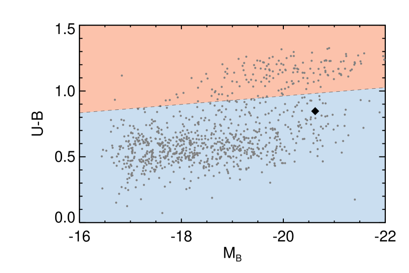
Figure 2.— A rest-frame color-magnitude diagram of galaxies in the redshift slice $0.3<z<0.4$ from the DEEP2 survey (grey points; Coil et al., 2004). The companion galaxy of the J2049-0012 system (z=0.37) is represented by a black diamond. It appears in the ‘green valley” between the main loci of the blue cloud and red sequences. The dotted line marks the separation between the red sequence and blue cloud as established by Willmer et al. (2006).

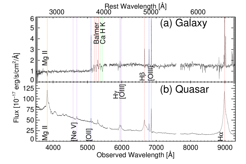
Figure 3.— One dimensional Keck/LRIS spectra of the galaxy and quasar comprising our interacting pair (the J2049$-$0012 system). Note the strong Balmer series absorption lines in the galaxy spectrum; these are suggestive of a starbust population. Also note that the quasar and galaxy are at nearly identical redshift. The quasar is at $z_{\rm q}=0.3691\pm 0.001$ and the companion galaxy is offset by only $160\pm 20$ ${\rm km~{}s^{-1}}$. As a clarification, we note that this quasar velocity is not the systemic velocity of its host galaxy. We find the velocity difference between the two galaxies to be $30\pm 30$ km/s. The strongest absorption and emisson lines are labelled by their ion. Fig. 10 shows an enlarged view of the post-starburst features along with models used to constrain the age of the stellar population.

Morphological analysis of the two objects is difficult. Firstly, the quasar (combined with its host galaxy) is consistent with a point source. The companion galaxy, meanwhile, is resolved with only a few spatial elements (observed to have FWHM of 1.86” [9.5 kpc] when our seeing was $\approx 0.64^{\prime\prime}$) and is also consistent with having an axis ratio of 1. Following Lotz et al. (2008a) and Conselice (2003), we measure a concentration for the companion galaxy of $C=5\log_{10}\left(\frac{r_{80}}{r_{20}}\right)$ where $r_{80}$ is the radius containing 80 percent of the total light, $r_{20}$ is similarly the radius containing 20 percent of the total light, and we have defined the total light to be the light within 1.5 times the Petrosian radius. We find that the galaxy has a concentration of 2.61 classifying it as a spiral (the standard dividing line is spirals have $C<3$). However, we note that since $r_{20}$ is within one seeing element, our measured concentration is only a lower limit and therefore the profile may actually be more consistent with an elliptical or bulge dominated system with a higher concentration. Around both galaxies there is some hint in the deeper R-band exposure of tidal debris, but since those regions did not fall into our slit we have no spectroscopic information about them and it is difficult to determine if this emission is truly associated with the galaxy or only close in projection (see Fig. 1).

Table 2 lists photometry for the two objects compiled from a variety of surveys, spanning UV to near-IR frequencies.

Examination of the photometric redshifts of nearby galaxies reveals no obvious overdensity at the quasar’s redshift. We examined this by looking at the number of objects within 1 Mpc projected distance from the QSO with consistent photometric redshifts ($1.5\sigma$) measured for 1000 random positions in the SDSS footprint that contained at least a single galaxy (at any redshift). The quasar appears in the low end of this distribution and hence there is no evidence for the quasar being in a rich and large cluster.

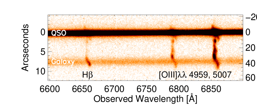
Figure 4.— 2D discovery spectrum of the J2049-0012 quasar/galaxy system centered near H$\beta$ and [O III] emission made using the Keck/LRIS 600/7500 grating. The continuum light of the quasar (top) and galaxy (bottom) are the bright horizontal bands in the image. The bright quasar spectrum is centered at the 0 kpc (0^′′) spatial position and saturates the image in this stretch. The image covers, from left to right, the H$\beta$, [O III]$\lambda 4959$, and [O III]$\lambda 5007$ transitions corresponding to $z=0.37$. These emission lines are detected for the quasar, its host galaxy, and the companion galaxy as well as a ‘bridge’ of emission that connects the two objects. The emission lines are not detected beyond the spatial slice presented here.

3.2. 1D Spectra of the QSO Host and Companion

The discovery spectrum was taken with the original goal of confirming this system as a projected background/foreground, quasar/galaxy system separated by a cosmological distance. We observed the objects using the Keck/LRIS spectrometer with its 1^′′ long slit aligned across the pair. Fig. 3 shows the fluxed 1D spectra. The quasar shows strong and broad H$\beta$ and Mg II emission lines confirming its SDSS classification and redshift. A Gaussian fit to the [O III] emission lines gives $z_{\rm q}=0.3691\pm 0.001$ which is within the errors of the SDSS measured redshift of $0.3693\pm 0.0015$. The broad emission lines appear unusually asymmetric.

The companion galaxy’s photometric redshift placed it well in front of the quasar, however the spectrum reveals the galaxy has strong emission and absorption features at nearly the identical redshift of the quasar with only a $\delta v\approx 150$ km/s second offset (Fig. 3). The spectrum is notable for strong emission lines characteristic of photoionization together with strong Balmer series absorption lines that indicate a moderate-aged stellar population ($t_{\rm age}\gtrsim 100$ Myr). The absorption lines may suggest that the galaxy has recently undergone a ‘burst’ of star-formation that may now be fading. After O and B stars die after $\sim$100 Myr, A stars remain a significant contributor to the stellar light until their death approximately 1 Gyr later. Type A stars provide characterisitic Balmer series absorption lines that make them easy to distinguish from other stellar types. If there is an older stellar population ($t>1$ Gyr) contributing to the galaxy light, the K giants will show strong Ca H+K absorption lines (Dressler & Gunn, 1983). The galactic spectral type that is characterized by both Balmer absorption lines and Ca H+K lines and with no emission lines is commonly referred to as K+A post-starburst, a relatively rare phase for galaxies especially at low redshift (Wild et al., 2009). These indicators suggest that the galaxy’s star formation rate is fading and/or has recently shut off. A common scenario used to explain such a signature is a passively evolving stellar population that underwent a burst of star formation that has recently subsided (Dressler & Gunn, 1983). Such bursts may be caused by tidal interactions in a merging galaxy system (Snyder et al. in prep.; Mihos & Hernquist, 1996). This applicability of this interpretation for our system is further discussed in $\S$5.2.3.

Because the galaxies are at nearly the same redshift, there is little information that can be used to determine which galaxy is foreground. Mg II absorption is clearly visible in the companion galaxy’s spectrum, while none is evident in the spectrum of the quasar (See Fig. 3). This could indicate that the companion galaxy is background to the quasar host galaxy (e.g. Rubin et al., 2010). However, the similar velocities of the two galaxies precludes one from unambiguously associating the gas with either the quasar host or the companion galaxy.

3.3. 2D Spectrum

In Fig. 4, we present a slice of the co-added, 2D discovery spectrum of the system centered near the observed H$\beta$ and [O III] emission lines. There are two sources with visible continua which appear as horizontal lines in this 2-dimensional spectrum: the quasar and the companion galaxy. The [O III] and H$\beta$ lines exhibit faint emission oriented at $\approx 20^{\circ}$ counter clockwise from vertical that extends $\approx 2^{\prime\prime}$ (10 $h_{72}^{-1}\,\rm kpc$) away from the spatial location of the quasar in directions both towards and away from the companion galaxy. We associate this emission with the underlying host galaxy of the quasar. The weaker continuum source located at impact parameter $\rho\approx 8^{\prime\prime}$ (38 $h_{72}^{-1}\,\rm kpc$) and its associated emission lines are from the companion galaxy. The galaxy emission shows obvious signatures of rotation; the [O III] emission spans $\sim$5 Å corresponding to $\Delta v=c\Delta\lambda/\lambda\approx 300\ {\rm km~{}s^{-1}}$ which implies a rotation speed $v_{\rm rot}>100{\rm km~{}s^{-1}}$. Interestingly, the galaxy’s emission properties vary as a function of spatial distance from the quasar: H$\beta$ emission is stronger on the side away from the quasar than the side toward it, while [O III] shows the opposite trend.

Of greatest interest to this work is the detection of a ‘bridge’ of emission that connects the quasar and galaxy. The bridge is strongest in [O III] but H$\beta$ and other lines shown in Fig. 6 are also positively detected. It appears that the bridge lies roughly along a line connecting the spatial and velocity centers of the two galaxies. Fig. 4 also reveals that along the line connecting the quasar and galaxy, the emission is confined to the space between them. In this respect, the emission differs from the EELRs commonly observed around quasars (e.g. Fu & Stockton, 2009), i.e., it appears to be directly related with the gas in this interacting system. To explore this point further, we obtained an optical spectrum with the Kast spectrometer on the 3m Shane telescope at Lick Observatory with the long slit centered on the bridge but oriented perpendicular at a PA perpendicular to that of our Keck/LRIS spectrum. By fitting a gaussian to the Kast spectrum, we found its FWHM=2.0^′′, which was consistent with our seeing limit for the night. Therefore we constrain the spatial extent of the bridge to be $<10.2\ h_{72}^{-1}\,\rm kpc$ perpendicular to the line connecting the quasar and companion galaxy.

3.4. Summary

Fig. 5 presents a cartoon of the inferred layout of the system. Taken altogether, the observations of this system suggest the following scenario: we are observing a pair of merging galaxies that have undergone an interaction which has tidally stripped material from at least one of the galaxies. This is suggested by the nearly identical redshifts of the galaxies and the presence of the bridge connecting the two galaxies. Such material is a standard prediction in theoretical models of gas-rich galaxy encounters (Toomre & Toomre, 1972a; Mihos & Hernquist, 1996) as well as a commonly observed phenomenon in nearby, interacting galaxies (e.g. Arp, 1966; Hibbard et al., 2001). The ongoing merger could have triggered a burst of star-formation in one (or both) of the galaxies and AGN activity in the galaxy now observed to be in a quasar phase. The companion galaxy appears to be in the ‘green valley’ and has a possibly fading starburst stellar population. This population is consistent with a starburst that was caused during the first passage of a galaxy interaction and may indicate that the galaxy is likely undergoing a substantial change in its stellar light properties. The fact that the higher ionization state lines are brighter closer to the quasar ($\S$4.2) suggests that the quasar is shining on the tidal material, photoionizing the majority of that gas. If this hypothesis is correct, then the full toolbox of low density astrophysics allows us to interpret observations of the bridge’s emission lines to give insights into the tidal material’s dynamics, column density, mass, temperature, metallicity, and volume density. In the following sections we test this physical interpretation of the system and its implications.

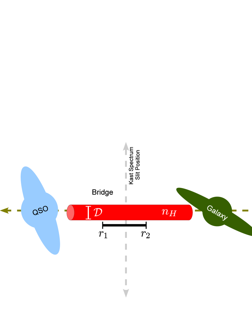
Figure 5.— A cartoon depiction for the assumed geometry of the J2049$-$0012 system. We assume that the bridge forms a cylinder of diameter $\mathcal{D}$ connecting the quasar host galaxy to the companion galaxy. $r_{1}$ and $r_{2}$ are radial distances from the quasar. The volume density of hydrogen is assumed to be a constant $n_{H}$. Also noted are the approximate slit positions of both the Keck/LRIS and Shane/Kast spectra. Using this simple model, we can estimate properties of the bridge including its volume and column densities and its mass.

4. Emission Line Measurements

The flux measurements and line ratios constrain properties of the gas and galaxies involved in this system. The kinematics provide estimates for the masses of the galaxies and give information about the merger stage and geometry. We present the emission line fluxes in Table 3. Inspection of Fig. 6 reveals that the emission line fluxes and the line ratios vary along the slit hence we have broken the bridge into three bins (0b, 1b, and 2b) and the galaxy into two equally sized bins (3g and 4g) as labelled in Fig. 6. The bounds of the regions noted as “bridge” and “galaxy” are determined by eye through inspection of the kinematic profiles. In the higher resolution spectrum, it is clear that the bridge has distinct kinematic characteristics from either galaxy.

Table 3Emission Line Measurements

	Region	Flux	Dereddened Flux	$\frac{Flux}{F_{5007}}$
		$10^{-17}\,\mbox{erg/s/cm}^{2}$	$10^{-17}\,\mbox{erg/s/cm}^{2}$
[N II]$\lambda$6585	0b	$<$0.87	$<$0.99	$<$0.07
	1b	1.34$\pm$0.38	1.52$\pm$0.43	0.12$\pm$0.03
	2b	$<$1.29	$<$1.46	$<$0.05
	3g	11.68$\pm$0.60	13.28$\pm$0.68	0.27$\pm$0.01
	4g	13.42$\pm$0.67	15.26$\pm$0.76	0.75$\pm$0.04
H$\alpha$	0b	4.89$\pm$0.43	5.56$\pm$0.49	0.38$\pm$0.04
	1b	3.53$\pm$0.50	4.02$\pm$0.57	0.31$\pm$0.04
	2b	5.19$\pm$0.56	5.90$\pm$0.64	0.22$\pm$0.02
	3g	32.51$\pm$0.77	36.98$\pm$0.88	0.77$\pm$0.02
	4g	38.18$\pm$0.79	43.44$\pm$0.89	2.14$\pm$0.08
[N II]$\lambda$6549	0b	$<$0.92	$<$1.04	$<$0.07
	1b	$<$1.18	$<$1.35	$<$0.10
	2b	$<$1.32	$<$1.50	$<$0.06
	3g	4.48$\pm$0.60	5.10$\pm$0.68	0.11$\pm$0.01
	4g	4.95$\pm$0.64	5.64$\pm$0.73	0.28$\pm$0.04
[O III]$\lambda$5007	0b	11.87$\pm$0.30	14.62$\pm$0.37	$\cdots$
	1b	10.65$\pm$0.35	13.11$\pm$0.44	$\cdots$
	2b	21.85$\pm$0.41	26.90$\pm$0.51	$\cdots$
	3g	39.24$\pm$0.55	48.30$\pm$0.67	$\cdots$
	4g	16.52$\pm$0.53	20.34$\pm$0.65	$\cdots$
[O III]$\lambda$4959	0b	4.27$\pm$0.26	5.27$\pm$0.32	0.36$\pm$0.02
	1b	3.70$\pm$0.31	4.57$\pm$0.39	0.35$\pm$0.03
	2b	7.41$\pm$0.36	9.14$\pm$0.44	0.34$\pm$0.02
	3g	12.93$\pm$0.48	15.96$\pm$0.60	0.33$\pm$0.01
	4g	4.77$\pm$0.46	5.89$\pm$0.57	0.29$\pm$0.03
H$\beta$	0b	1.30$\pm$0.25	1.62$\pm$0.32	0.11$\pm$0.02
	1b	1.72$\pm$0.31	2.14$\pm$0.38	0.16$\pm$0.03
	2b	2.40$\pm$0.34	2.97$\pm$0.43	0.11$\pm$0.02
	3g	9.51$\pm$0.47	11.81$\pm$0.58	0.24$\pm$0.01
	4g	8.18$\pm$0.46	10.15$\pm$0.57	0.50$\pm$0.03
[Ne III]$\lambda$3869	0b	0.92$\pm$0.22	1.22$\pm$0.29	0.08$\pm$0.02
	1b	1.05$\pm$0.25	1.39$\pm$0.33	0.11$\pm$0.03
	2b	1.68$\pm$0.28	2.22$\pm$0.37	0.08$\pm$0.01
	3g	4.08$\pm$0.37	5.41$\pm$0.49	0.11$\pm$0.01
	4g	2.00$\pm$0.36	2.65$\pm$0.47	0.13$\pm$0.02
[O II]$\lambda$3727	0b	1.18$\pm$0.21	1.59$\pm$0.28	0.11$\pm$0.02
	1b	$<$0.72	$<$0.96	$<$0.07
	2b	2.00$\pm$0.26	2.69$\pm$0.35	0.10$\pm$0.01
	3g	12.83$\pm$0.52	17.21$\pm$0.70	0.36$\pm$0.02
	4g	14.30$\pm$0.49	19.19$\pm$0.65	0.94$\pm$0.04
[Ne V]$\lambda$3426	0b	2.44$\pm$0.20	3.38$\pm$0.28	0.23$\pm$0.02
	1b	2.18$\pm$0.23	3.03$\pm$0.32	0.23$\pm$0.03
	2b	2.26$\pm$0.25	3.14$\pm$0.35	0.12$\pm$0.01
	3g	1.24$\pm$0.32	1.73$\pm$0.44	0.04$\pm$0.01
	4g	$<$0.94	$<$1.30	$<$0.06
[Ne V]$\lambda$3346	0b	0.92$\pm$0.20	1.28$\pm$0.28	0.09$\pm$0.02
	1b	0.79$\pm$0.23	1.10$\pm$0.33	0.08$\pm$0.03
	2b	$<$0.71	$<$1.00	$<$0.04
	3g	$<$0.96	$<$1.35	$<$0.03
	4g	$<$0.96	$<$1.35	$<$0.07

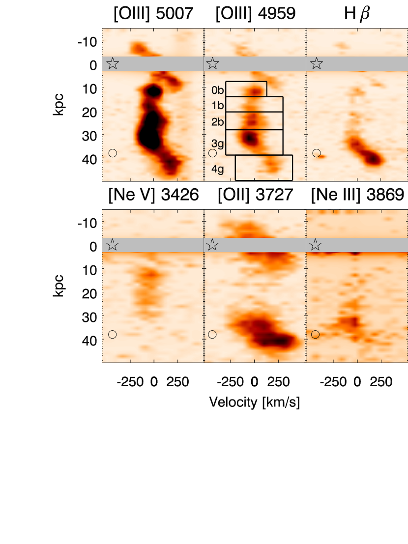
Figure 6.— Portions of the discovery spectrum taken with Keck/LRIS on 2008-10-03 after continuum subtraction. The star denotes the spatial position of the quasar and the open circle marks the position of the companion galaxy. A grey bar has been placed over the core of the quasar to aid the eye. These images have been interpolated to be on the same spatial and velocity grid. The [O III]$\lambda 4959$ panel shows the spatial boxes used throughout the paper which separates regions in each of the bridge (0b, 1b,2b) and the companion galaxy (3g,4g).

4.1. Line Fluxes

To properly isolate the emission line fluxes, we needed to first subtract the continuum light from the quasar and the galaxy. This required construction of an accurate model of the flux from each object. We took the 2-dimensional profile fits from Low-Redux (interpolating over the emission-line regions) and multiplied by the 1-dimensional boxcar extraction. An additional complication arises from the companion galaxy’s Balmer absorption lines. To account for these spectral features, we used the stellar population model described in $\S$ 5.2.3, to model the absorption for the H$\alpha$ and H$\beta$ fluxes. This resulted in a spectrum containing only the emission lines (Fig. 6).

The main contributions to the error are the statistical errors of the signal (Poisson errors) and the errors associated with our data reduction (i.e. sky subtraction and continuum subtraction). While the former is relatively straightforward to estimate, the latter is more difficult. We estimated this systematic error through analysis of our science images that had been sky and profile subtracted as follows. For every pixel in these images, we calculated the sigma-clipped mean and standard deviation in a square region with 10 pixels on a side (after masking known cosmic rays and the emission lines themselves). We then have an image of the local means and an image of the local standard deviations. For each emission line we picked a region from these images of means and standard deviations that is nearby (but does not include emission) and proceeded to take their averages. We then add an additional error term in quadrature with the Poisson errors equal to the average of the standard deviations in this region. We also include an additional error associated with over/undersubtracting the profiles that is characterized by applying the entire profile subtraction algorithm to regions that contain no emission lines and measuring fluxes in the same velocity apertures in those regions.

Lastly, when comparing line fluxes we must take care to consider the same spatial region for each of the emission lines. Because our observations were taken with different cameras each with a different plate scale, the spatial region determined by an integer number of pixels for one of the plate scales is not generally equal to an integer number of pixels for others. Therefore, we insure we are comparing the same region by interpolating the spectrum onto a grid 100 times finer in spatial and velocity resolution. We note that this is valid as our platescales, seeing, and dispersion render the data Nyquist sampled in all of the observations. We then use the spatial centroid of the quasar continuum light as a reference and extract along the same spatial intervals for all the lines. We then apply velocity extraction windows as shown in Fig. 6. The velocity extraction windows are broader for the [O II] lines because they form a doublet and are treated as a single line which is therefore seen to have a larger velocity spread. The H$\alpha$ and [N II] lines have slightly smaller velocity windows to prevent overlap with nearby bright skylines.

The flux measurements are presented in Table 3. We corrected fluxes for Galactic foreground reddening using the Schlegel, Finkbeiner and Davis dust maps ($A_{V}=0.292$; Schlegel et al., 1998) and a Milky Way dust extinction curve from Cardelli et al. (1989).

4.2. Line Ratios

Fig. 7 presents several line ratios that gauge physical characteristics of the system. One such ratio, that of H$\alpha$ to H$\beta$ (black crosses), is a standard indicator of dust absorption. The dotted lines show theoretical estimates of this ratio at a range of temperatures spanning reasonable expectations for photoionized gas (Osterbrock & Ferland, 2006). The agreement between the observations and theoretical prediction implies that there is little dust in the bridge and only modest extinction within the companion galaxy.

The figure also shows how the brightness of an emission line varies with distance from the quasar. The apparent trend is that lines coming from higher ionization species reach their brightest intensities (relative to other lines) closer to the quasar while lower ionization species show the opposite trend. Thus the ratios [O III]/H$\beta$, [Ne V]/[Ne III], and [Ne V]/[O III] are decreasing with increasing distance from the quasar. This suggests that the quasar is related to the observed emission (see $\S$ 6.2).

The ratio of [Ne V] to [Ne III] constrains the ionization parameter of the gas (which is an indicator of the ionization state of the gas). Indeed, the presence of [Ne V] emission alone requires a source of high energy photons or high temperature ($T$) gas (with an ionization potential exceeding 7 Rydberg, H II regions will not typically produce this line). The emission line ratios are also important in determining the source of ionization, e.g. [N II]/H$\alpha$ and [O III]/H$\beta$ are sensitive to the ionizing source’s spectrum.

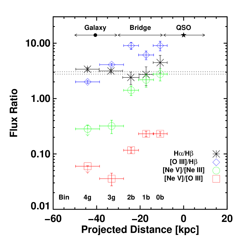
Figure 7.— The spatial variation of various line ratios measured for the J2049$-$0012 system. The lines used were H$\alpha$, H$\beta$, [O III]$\lambda$5007, [Ne V]$\lambda$3426, and [Ne III]$\lambda$3869. The dotted lines denote the theoretical values for the H$\alpha$/H$\beta$ ratio for gas at $T_{e}=5,000$K (3.05) and at 20,000K (2.76) (Osterbrock & Ferland, 2006). The galaxy and bridge are consistent with having little intrinsic dust. Higher ionization lines are stronger relative to lower ones closer to the QSO (at spatial position 0 kpc). This trend suggests that it is possible the quasar is responsible for the emission because the [O III]/H$\beta$, [Ne V]/[Ne III], and [Ne V]/[O III] ratios are all sensitive to the ionization state of the gas.

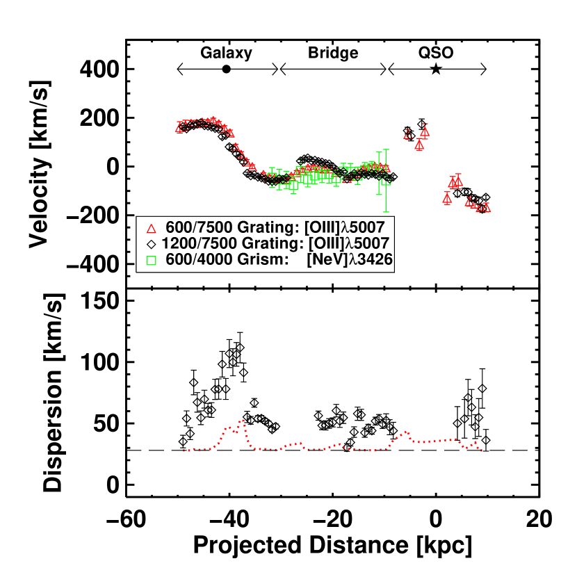
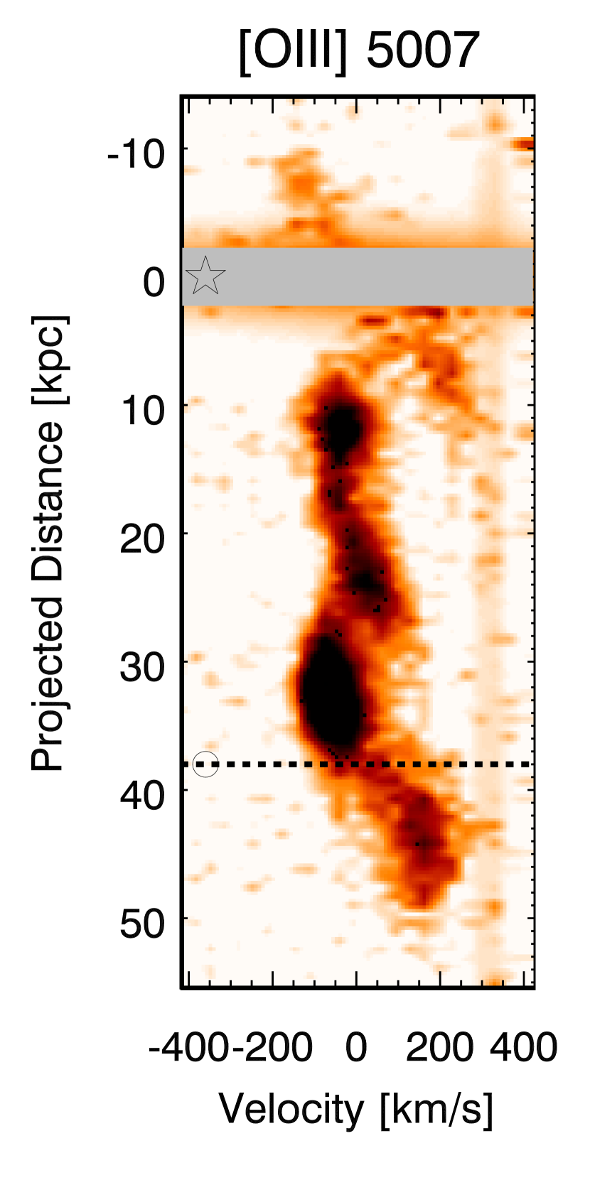
Figure 8.— Kinematic characteristics for several emission lines detected for the J2049$-$0012 system. The values presented on the left are derived from Gaussian fits to each spatial row in the 2D spectrum. (left top) The velocity centroids of each fit; 0 km/s is defined by the SDSS redshift of the QSO. The arrows at the top denote the spatial extent of each region of the system. Specifically, the star denotes the centroid of the quasar, the circle the centroid of the galaxy and the central region is called the bridge. Note that the [Ne V] emission is kinematically coincident with the [O III] emission indicating that these ions likely arise in a single phase of gas. (left bottom) The velocity dispersions ($\sigma$) measured from the higher resolution 1200/7500 grating for the [O III]$\lambda$5007 line. The dashed line is the measured velocity dispersion of a nearby sky line. The red dotted line represents the expected velocity dispersion as expected by the finite spatial resolution of the spectrum (see the text). Spatial bins that were poorly fit by a single gaussian have been masked. (right) The higher resolution (1200/7500 grating) spectrum of the [O III] emission. This spectrum shows finer detail than the 600/7500 grating and is used for comparisons with simulations and to estimate the masses of the galaxies. One can clearly see that the bridge has distinct kinematic properties from either galaxy, yet connects spatially with each galaxy near their velocity centroids.

4.3. Kinematics

The kinematics of the emission constrain the driving gravitational forces on the gas. They also provide estimates for the masses of both the QSO host and its companion galaxy. Coupled with comparisons to simulations, we can also learn about the specific merger stage of the galaxies. To characterize the kinematics of the ionized gas, we calculated the flux-weighted velocity centroid and velocity dispersion in the [O III]$\lambda 5007$ line within each spatial row of pixels. We choose the [O III]$\lambda 5007$ line because it is the brightest observed line with the highest signal-to-noise ratio. These measures were calculated by fitting single gaussians to all velocity pixels corresponding to a given spatial row of pixels. Each fit was checked by eye and catastrophic errors related to non-gaussian line-profiles have been masked. These are due to regions with low signal-to-noise or when there are overlapping velocity components (e.g., in spatial regions that include both the bridge and one of the galaxies).

The dominant source of uncertainty in these kinematic measures is related to systematic effects. Specifically, the wavelength solution based on the arc lamp images has a typical RMS residual of $\approx 0.1$ pixels corresponding to a velocity of $\approx 10\ {\rm km~{}s^{-1}}$. The systematic velocity error due to this effect is calculated for each line by (1) measuring the RMS of the residuals from our wavelength solution in units of pixels (2) multiplying the RMS by the dispersion (Å/pix) to get the wavelength RMS (3) then estimating the error that is introduced at each line’s observed wavelength. These errors are added in quadrature with the fitting errors.

We find that the kinematics of the [Ne V]$\lambda 3426$ line trace the [O III]$\lambda 5007$ emission; it is thus very likely that these ions are co-spatial. This is a crucial point for the determination of the ionization source, as it allows us to demand that the same ionization mechanism produce each of these ions and their observed line ratio.

The velocity centroids and dispersions ($\sigma$) of [O III]$\lambda 5007$ as measured from our highest resolution R1200/7500 observation are shown in Fig. 8. In our higher resolution spectrum, the kinematics of the gaseous bridge appear distinct from the rotation observed in the quasar’s host galaxy and the companion galaxy (See Fig. 8).

The lower panel reports the measured velocity dispersions of the 1200/7500 measurements of the [O III] $\lambda 5007$ line. The width of a nearby unresolved sky line is plotted as a dashed line to indicate the resolution limit of the spectrum. Since the velocity dispersions are higher than those of a nearby skyline we appear to have spectroscopically resolved the emission of the bridge, but it is unclear if we have done so spatially. Specifically, we emphasize that if there are spatial gradients in the velocity field that are unresolved they have the effect of artificially increasing the velocity dispersion because the gradient is smeared. Thus one might misinterpret spatially unresolved velocity shear as random motions. To quantify this effect we created a mock 2D spectrum with the same central velocities and brightnesses as a function of position as those measured from our data. To isolate the effects of this spatial smearing we set the velocity dispersions of each spatial pixel equal to that of the unresolved skyline. We then smoothed this 2D spectrum in the spatial direction according to a spatial resolution element of 0.7^′′ and measured the velocity dispersion in the same manner as for the data. The result is represented as the red dotted curve and can be interpreted as the expected effective resolution limit as a result of both finite velocity resolution and astronomical seeing. Since the velocity dispersion is still higher than this curve, it appears we are also spatially resolving the velocity dispersion (as long as the gradients are not smaller than the seeing).

The velocity of the quasar spectrum as measured from AGN emission lines is generally a poor measure of the systemic velocity for its host galaxy (e.g., Richards et al., 2002). Therefore, we have also analyzed the host galaxy’s extended [O III] emission. We use the measured centroids on either side of the host galaxy along with the spatial centroid of the quasar light to interpolate the velocity at the spatial center of the host galaxy. We do this by fitting a robust linear fit to the data. Thus we measure the relative radial velocities of the quasar host galaxy and companion galaxy to be $30\pm 30$ ${\rm km~{}s^{-1}}$, with the quasar at the higher radial velocity.

5. Physical Properties of the Interacting Pair

In this section we present analysis detailing measured physical properties of the galaxies and the SMBH of the QSO involved in the merger.

5.1. QSO Properties

One can estimate the mass of the supermassive black hole $M_{BH}$ fueling the quasar activity in several ways based on the emission line characteristics (Vestergaard & Peterson, 2006; Kong et al., 2006). By fitting SED templates one may estimate the bolometric luminosity of the QSO from the continuum luminosity in a particular wavelength region. The quasar under study is in the SDSS QSO catalog of Shen et al. (2008) who used the above methods to calculate $L_{Bol}=10^{45.7}$ erg/s and $M_{BH}=10^{8.7}M_{\odot}$ where each has a typical error of approximately 0.4 dex. This places the quasar above the average for quasars at this redshift but within approximately 1$\sigma$ of the distributions for both quantities. This also gives an Eddington ratio of 0.07 which falls within the normal range for quasars (Kelly et al., 2010).

We utilize the calibration of Ferrarese (2002) derived using Bullock et al. (2001) to estimate the dark matter halo mass of the QSO host galaxy,

$$\frac{M_{DM}}{10^{12}M_{\odot}} \approx 1.40\left(\frac{v_{c}}{200{\rm km~{}s^{-1}}}\right)^{3.32}\;\;\;,$$ (1)

where $v_{c}$ is the circular velocity of the host galaxy at the point where the rotation becomes flat.

Using the data from the R1200/7500 grism (see Fig. 8), we find that emission associated with the quasar host galaxy extends from $-174.3$ to +174.0 ${\rm km~{}s^{-1}}$ (where our measurements at the positive velocity end are truncated when they become cospatial with the bridge). These velocities however are relative to the SDSS quasar redshift and not the systemic velocity of the quasar host. Using the methods described in $\S$4.3, we found the offset to be $30\pm 30$ km/s. Thus we arrive at an estimate of $v_{c}\geq(200\pm 30)/\sin i$ where $i$ is the galaxy inclination. This is a lower limit on the actual circular velocity because (1) we may not have aligned our slit with the major axis of the galaxy and (2) our spectrum does not appear to extend to the flat portion of the rotation curve. Using the 1$\sigma$ error below the measured value, we find that this gives an estimate of the host mass to be $M_{DM}>8.8\times 10^{11}\ M_{\odot}$.

With IFU spectra or additional spectra at different slit angles, we could constrain the inclination and axis ratio of the host galaxy to better characterize the host galaxy’s dynamical mass. Space-based imaging however would allow us to directly image the host’s bulge and multiband imaging would allow us to better estimate its stellar mass. In paper II we discuss the position of the BH and host on Magorrian-like relations and details of how this and other systems like it might lead to insights on whether a host galaxy leads/lags its SMBH.

5.2. Companion Galaxy Properties

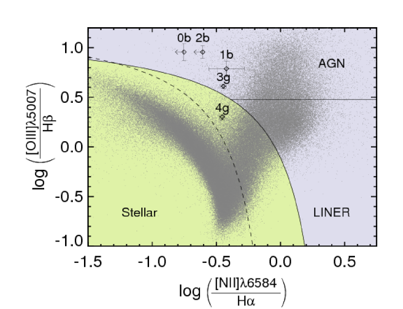
Figure 9.— A BPT (Baldwin et al., 1981) diagram of the flux ratios observed for the bridge (0b, 1b, 2b) and companion galaxy (3g, 4g) regions as demarcated in Fig. 6. The points are a random selection of galaxies from SDSS to give a sense of the normal locus of objects. The solid curve is from Kewley et al. (2001) and separates regions consistent with ionization from H II regions from other sources of ionization. The dashed curve is a similar division found by Kauffmann et al. (2003b). The horizonal line segment denotes the separation between LINERS and AGN (Veilleux & Osterbrock, 1987). The regions of the bridge (0b, 1b, 2b) are consistent with being photoionized by a hard AGN spectrum while bin 4g (located farthest from the quasar) is more consistent with H II regions. Bin 3g is in a portion of the diagram that is inconsistent with ionization by H II regions alone and likely has an ionizing spectrum that includes the AGN and a stellar component.

5.2.1 Star Formation Rate & Gas Metallicity

The observed line ratios of H$\alpha$/[NII] and [OIII]/H$\beta$ define the the standard axes of the Baldwin, Phillips and Terlevich (BPT) diagram (Baldwin et al., 1981, see Fig. 9). These line ratios are used because they are sensitive to the hardness of the spectrum and the temperature of the gas (which in turn is also sensitive to the hardness of the spectrum). Furthermore, these are bright lines in the optical passband that are closely spaced in wavelength such that differential reddening is generally negligible. In this diagram H II regions occupy a particular locus, while AGN and LINER sources each separate into their own loci. The curved line denotes the division between emission characteristic of ionization from hot young stars in H II regions from ionization from other sources (Kewley et al., 2001). The dashed curve is a similar division as reported by Kauffmann et al. (2003b). The horizontal line segment to the right of this curve at a value of $\log($[O III]$\lambda 5007/H\beta)=\log(3)$ denotes the division between the LINER and Seyfert line ratios as defined by Veilleux & Osterbrock (1987).

The galaxy spans bins 3g and 4g. While bin 3g appears strongly affected by an AGN-like source, bin 4g is closer to the locus of gas photoionized by stars. Under the hypothesis that the ionization in region 4g of the companion galaxy is consistent with H II regions, we can estimate the star formation rate using the Kennicutt (1998) calibrations for H$\alpha$:

$$SFR_{4}(M_{\odot}\textnormal{ yr}^{-1}) = 7.9\times 10^{-42}L(\textnormal{H}\alpha)(\textnormal{ergs s}^{-1})^{-1}$$ (2)

$$= 1.61\pm 0.03\ M_{\odot}\textnormal{ yr}^{-1}.$$

Assuming that the [OII] emission also arises from H II regions, we can additionally estimate

$$SFR_{4}(M_{\odot}\textnormal{ yr}^{-1})=(1.4\pm 0.4)\times 10^{-41}L([\mbox{{O~{}II}}])(\textnormal{ergs s}^{-1})^{-1}=1.25\pm 0.36\ M_{\odot}\textnormal{ yr}^{-1}.$$ (3)

The two estimates are in good agreement, suggesting that dust is not adversely affecting the line fluxes. Of course, we are not sensitive to any highly obscured star formation and in this sense the measured star formation rate is a lower limit. We also note that this SFR is only measured over bin 4g. We also detect H$\alpha$ emission for the galaxy within bin 3g but we expect that these line fluxes are influenced by the neighboring QSO’s ionizing radiation. Therefore, we assume that the star formation in that bin is equal to bin 4g and apply a multiplicative correction factor of 2. We also need to correct for the fact that our slit is only 1^′′ wide and the galaxy extends outside of the slit. To do this, we make use of our $R$-band image and (1) measure the total flux of the galaxy (2) apply a 1^′′ slitmask and measure the total flux which falls within this slit. The ratio of these two fluxes is the slit loss correction. We find this to be a factor of 2.5. We thus apply a total correction factor of 5. This of course is assuming that the star formation rate is constant across the entire galaxy and that the $R$-band light follows the star formation. This gives an estimate of the total star formation rate for the galaxy of $8.05\pm 0.15M_{\odot}\mbox{ yr}^{-1}$.

As a caveat, we point out that the star formation in the companion galaxy may be dominated by its innermost regions and thus not indicative of the overall galaxy morphology. This may occur when gas is funneled by tidal torques of the interaction to trigger a burst of recent star formation. If this is the case, we may be overestimating the slit loss correction. For a tabulated summary of all SFR estimates with the varying assumptions, see Table 4. These estimates likely bracket the range of possible star formation rates.

We may also estimate the metallicity of the gas in bin 4g using standard line flux ratio calibrations. Pettini & Pagel (2004) outline two calibrations of metallicity determination. In these units solar O/H is 8.66 (Allende Prieto, Lambert, & Asplund, 2001; Asplund et al., 2004):

$$12+\log(\mbox{O/H}) = 8.9+0.57\times N2=8.64\pm 0.01$$ (4)

$$12+\log(\mbox{O/H}) = 8.73-0.32\times O3N2=8.49\pm 0.01$$ (5)

where $N2\equiv\log\{[$N II$]/\mbox{H}\alpha\}$ and $O3N2\equiv\log\{\left([\mbox{{O~{}III}}]/\mbox{H}\beta\right)/\left([\mbox{{N~{}II}}]/\mbox{H}\alpha\right)\}$. These empirical relations have scatter such that 95% of points are within 0.38 dex of the $N2$ calibration and within 0.25 dex of the $O3N2$ calibration. Thus the two measurements are in agreement within the systematics of each other and the solar value. Therefore, we conclude that the galaxy has roughly solar metallicity.

5.2.2 Mass Estimates

We can estimate the mass of the companion galaxy in the same manner as for the quasar host galaxy ($\S$5.1), i.e., through analysis of the rotation curve. The measured circular velocity implies an estimate to the dark matter halo mass $M_{DM}>2.1\times 10^{11}M_{\odot}$. This is also a lower limit due to uncertainties in the inclination, axis ratio, and position angle of the galaxy. We note, however, that unlike the quasar host, the data does extend to the flat portion of the rotation curve.

Using the 5 SDSS colors ($ugriz$), one may constrain the spectral energy distribution of a galaxy at $z<1$ to estimate its mass-to-light ratio. This mass-to-light ratio can then be combined with the observed luminosity to estimate its stellar mass. Making use of version v4.1.4 of the kcorrect code (Blanton & Roweis, 2007), we estimate a stellar mass of $1.9\times 10^{10}M_{\odot}$ with a typical error of approximately 0.2 dex compared to other photometric estimates of stellar mass. Using the calibration of Conroy & Wechsler (2009) which is very similar to that of Fontana et al. (2006), we find that $M^{*}(z=0.369)=1.01\times 10^{11}M_{\odot}$. Therefore, the companion galaxy appears to be $\approx 0.2M^{*}$. Using halo abundance matching to relate stellar mass to halo mass (e.g. Conroy & Wechsler, 2009), we estimate the dark matter halo mass to be approximately $6\times 10^{11}M_{\odot}.$

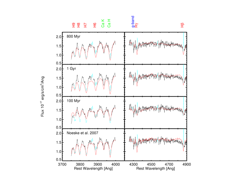
Figure 10.— Comparison of SSP models to the observed spectrum. Data are shown in black, the models are shown in red, and masked emission line regions are shown in cyan. The observed strong Balmer absorption lines are characteristic of A star features which indicate star formation halted in a time period that is longer than the lifetime of O and B stars but shorter than that of A stars. This range is 100 Myr - 1 Gyr and we refined the age estimate with SSP modeling. We find that the range of reasonable models is for starbursts that started t=300-800 Myr ago. Older stellar populations do not have strong enough Balmer features and are too red. Younger populations also underestimate the Balmer features and are too blue. Our best model is plotted in the first row which corresponds to 800 Myr. The second and third rows show examples of the poor fits that result from too old and too young populations respectively. We also show in the bottom panel the results of using a star formation history determined by Noeske et al. (2007). This SFH insufficiently reproduces the spectral region between Ca K and H7.

5.2.3 Stellar Population Models: Is the Companion a Post-Starburst Galaxy?

The classic definition of a post-starburst galaxy is one which has strong Balmer absorption features along with Ca H+K absorption lines and an absence of emission lines. While our galaxy does have emission lines which point to ongoing star formation, we believe that our galaxy falls into the post-starburst class for two reasons: (1) a significant portion of the emission may be a result from photoionization from the nearby quasar and (2) our following analysis demonstrates that the star formation was likely elevated in the past in order to simultaneously reproduce the colors and absorption lines.

We utilize Bruzual & Charlot (2003) population synthesis models to constrain the star formation history of this galaxy. We construct solar metallicity models using Padova 1994 stellar evolutionary tracks with a Chabrier (2003) IMF. Following Yan et al. (2006), we used various two-component models for the burst star formation history. The first component is a single 7 Gyr old, instantaneous stellar population which represents an old passively evolving background stellar population. The second component is a $\tau$ model burst occurring within the last 2 Gyr. We used a variety of $\tau$’s to parameterize our burst of star formation [where $SFR\propto\exp(-t/\tau)$]: 0.01, 0.1, 0.25, 0.5, 0.75, 0.9, 2, and 4 Gyr and spaced the age of the burst at 100 Myr intervals. We allowed a range of burst amplitudes ($A$; defined in the same manner as Kauffmann et al. (2003a)) such that the stellar mass produced by the burst (evaluated at $t=\infty$) relative to the initial 7 Gyr population was between $10^{-3}$ and $10^{4}$ in logarithmic steps of $\Delta\log A=0.53$.

We fit these model spectra to match our observed spectrum after correcting for Milky Way dust absorption in the same manner we treated our emission flux measurements (see $\S$ 4.1). Due to the LRIS dichroic gap we restricted ourselves to two rest wavelength ranges $3700-4000$ Å and $4250-4900$ Å. We also masked all pixels within 400 km/s of an emission line since our models do not include nebular emission. We allowed the model spectrum to scale up or down by a single constant factor and allowed for an intrinsic dust correction. The dust correction was implemented with a Charlot & Fall (2000) law parameterized by $\tau_{V}$:

$$F_{\lambda,obs}=F_{\lambda,int}\ \textrm{ exp}\left[-\tau_{V}\left(\frac{\lambda}{\mbox{5500 \AA}}\right)^{-0.7}\right]$$ (6)

where $F_{\lambda,obs}$ is the observed flux and $F_{\lambda,int}$ is the intrinsic flux.

We applied the additional criterion that the SDSS $u-g$, $g-r$, $r-i$, and $i-z$ colors of the models (including applying the Milky Way dust absorption and fitted intrinsic dust) are within 0.5 mag of the observed colors.

Altogether, we created 2016 models. We find that no individual model provides a good ($\chi^{2}_{r}=1$) fit to all of the spectral features. However the models that simultaneously best reproduce the observed colors and the line features (both the Balmer and Ca H+K) have ages for the burst component that fall in the range of 300 - 800 Myr, star formation histories parameterized by 0.25 Gyr $<\tau<$ 0.9 Gyr, and have a burst mass fraction (relative to the old passively evolving component) that fall in the range 0.009-0.1 (see Fig. 10). However we note that among those models there are a handful which have a mass fraction as high as 4. All models have dust reddening characterized by $\tau_{V}<1.01$ with very few having $\tau_{V}>0.7$. The best model has $\tau_{V}=0$, consistent with the observed H$\alpha$/H$\beta$ ratio (Figure 7). Older models are too red, while younger models are too blue. Higher burst fractions underestimate Ca H+K and g-band absorption features while lower burst fractions have insufficient Balmer features or too red colors. In summary, we find the data are best described by a substantial burst that occurred 800 Myr ago and that models with $t<300$ Myr and $t>800$ Myr are disfavored.

A reasonable question to ask is whether the companion galaxy is consistent with a normal, non-burst galaxy. To do this we make use of the star formation histories derived by Noeske et al. (2007) for star-forming galaxies at the redshift of our system. They present parameters of $\tau$ model star formation histories as a function of baryonic mass. We have an estimate of the stellar mass of the galaxy (see above) which we assume to be the baryonic mass of the galaxy; corrections to include gas up to reasonable gas fractions ($\lesssim 50\%$) have little to no effect on the following results. Thus, we find the star formation parameters to be $\tau=25.06$ Gyr and after converting from redshift intervals to ages, we find the beginning of the model be $5.13$ Gyr prior to our current observation of the galaxy. Thus this model is very nearly a constant star formation rate model. We fit this model to the data allowing for a normalization factor and dust reddening as we did for the burst models. We present the results in the bottom panel of Fig. 10. One can see that this model insufficiently produces the spectral features between Ca K and H7. Additionally, the model’s large amount of ongoing star formation produces too blue of an SED and thus requires a rather large column of dust to redden the spectrum ($\tau_{V}=1.27$). Assuming the same amount of reddening corresponds to the H II regions that we use to estimate the SFR, we find two results. Firstly, this measure of reddening implies a higher H$\alpha$/H$\beta$ ratio than observed, but only by $\gtrsim 1\sigma$. Secondly, the reddening correction would increase our estimate of the SFR by a factor of 3.7 giving a value greater than 20 $M_{\odot}/$yr. Comparison with the observational results of the specific star formation sequence (Noeske et al., 2007), we find this star formation rate lies well above the 84th percentile for galaxies at this stellar mass. These pieces of evidence argue against this scenario, but we cannot rule it out altogether.

The relatively high level of ongoing star formation may also be an indicator of a previous phase of elevated star formation. SFHs for galaxy mergers are not $\delta$-functions. For example, Cox et al. (2006) show that while the SF activity reaches a peak after first passage it can remain elevated until the merger ultimately coalesces.

6. Analysis of the Bridge

6.1. Density & Mass

We can make an order of magnitude estimate of the column density along the line of sight through the bridge by using the observed luminosity of the bridge in recombination lines combined with a simple volume model for the bridge (See Fig. 5). We note that the column density we are about to estimate is not the column density of material that the quasar radiation encounters along the bridge, but is the projected column on the sky from our perspective. We denote this column density as $N_{H,\perp}$ because if the bridge is in the plane of the sky then this column density is perpendicular to the column density that the quasar’s radiation encounters.

We start with the expression for the luminosity of the H$\alpha$ line produced by recombinations:

$$L_{\textrm{H}\alpha}=n_{e}n_{p}\alpha_{\textrm{H}\alpha}^{eff}Vfh\nu_{\textrm{H}\alpha}$$ (7)

where $L_{\textrm{H}\alpha}$ is the luminosity of H$\alpha$ in a given spatial region, $n_{e}$ is the number density of electrons, $n_{p}$ is the number density of protons, $\alpha_{\textrm{H}\alpha}^{eff}$ is the $\textrm{H}\alpha$ effective recombination coefficient, $V$ is the volume the gas fills, $f$ is the filling factor of the gas in that volume (observationally unconstrained but by definition $\leq 1$), $h$ is Planck’s constant, and $\nu_{H\alpha}$ is the frequency of the H$\alpha$ transition. We assume that the bridge is a cylinder with diameter $\mathcal{D}$ that extends a radial distance $r_{1}$ from the QSO to a larger radial distance $r_{2}$ (we note that $r_{1},r_{2}\gg\mathcal{D}$; see Fig. 5). In this case, $V\approx\mathcal{D}^{2}\left(r_{2}-r_{1}\right)$.

Assuming that the hydrogen is fully ionized, we take $n_{e}=n_{p}=n_{H}$, where $n_{H}$ is the number density of hydrogen in all ionization states. This is a reasonable assumption given the observed line ratios.

Manipulating eqn. 7 and substituting for our expression of $V$ we define:

$$\omega\equiv f^{1/2}n_{H}\mathcal{D}=\sqrt{\frac{L_{H\alpha}}{\left(r_{2}-r_{1}\right)\alpha_{H\alpha}^{eff}h\nu_{H\alpha}}}\approx 10^{21}\mbox{ cm}^{-2}.$$ (8)

This quantity consists only of observed quantities and atomic constants. The order of magnitude estimate is made using the observed flux of H$\alpha$ for bin 1b which we round to $4\times 10^{-17}$ erg/s/cm². Using the observations from bin 1b, we put a limit on the volume density of the gas by noting that:

$$n_{H}\approx\frac{\omega}{f^{1/2}\mathcal{D}}\approx 1\ f^{-1/2}\left(\frac{\mathcal{D}}{1\mbox{ kpc}}\right)^{-1}\mbox{ cm}^{-3}$$ (9)

Taking the limit to $\mathcal{D}$ placed by our Kast observations ($<$ 10 kpc), we derive $n_{H}\gtrapprox 0.1\ f^{-1/2}\mbox{ cm}^{-3}$. This is consistent with volume densities estimated for similar gaseous bridge structures in galaxy merger simulations by Weniger et al. (2009), where they implemented a multiphase ISM code in a galaxy merger simulation.

We may now estimate the column density,

$$N_{H,\perp} = \frac{\mbox{ $\#$ of Hydrogen atoms}}{\mbox{Surface Area those atoms fill}}\approx\frac{fn_{H}V}{\mathcal{D}\left(r_{2}-r_{1}\right)}$$ (10)

$$\approx n_{H}f\mathcal{D}\approx\omega f^{1/2}\approx f^{1/2}\ 10^{21}\mbox{ cm}^{-2},$$

This value is consistent with that of 21 cm neutral hydrogen observations of tidal tails of the Antennae galaxy by Hibbard et al. (2001). If that gas were fully ionized, then it would give rise to a similar column density of H⁺. Lastly, we estimate the hydrogen mass

$$M_{H} = n_{H}Vfm_{p}\approx\mathcal{D}\left(r_{2}-r_{1}\right)\omega f^{1/2}m_{p}$$ (11)

$$\approx 10^{8}\ f^{1/2}\left(\frac{\mathcal{D}}{1\mbox{ kpc}}\right)M_{\odot}.$$

This is relatively modest, but we note that $\mathcal{D}$ could be as large as 10 kpc although $f$ could also be significantly smaller than unity.

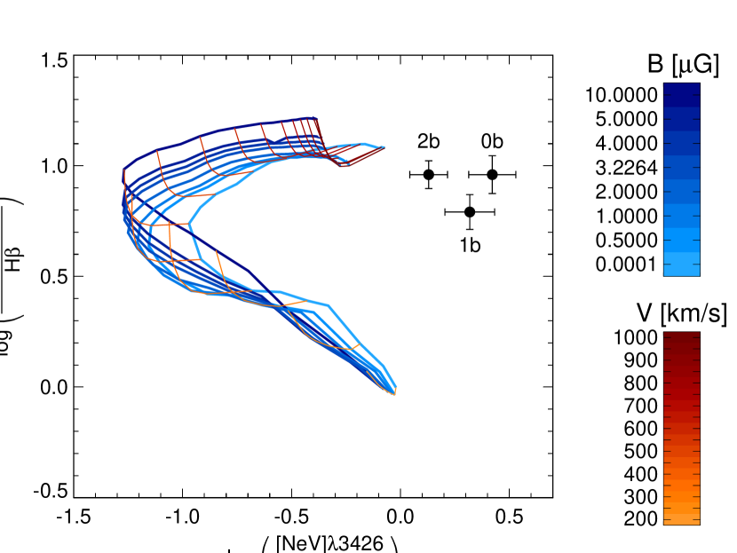
Figure 11.— Comparison of the predicted line ratios for fast, radiative shocks (curves; Allen et al., 2008) with the observed values in the bridge (bins 0b, 1b, and 2b). These predictions are for fast radiative shocks+precursor in gas with a density of 1 cm^-2 and solar metallicity. The range spanned by the predictions is relatively insensitive to these choices. The bridge’s emission is inconsistent with shocks even if we allow those shocks to be unreasonably fast (up to 1000 km/s).

6.2. Source of Ionization

We observe the bridge in emission lines from recombination of Hydrogen and forbidden lines of high ionization species. This, of course, requires a physical source of ionization and heating of the gas. In this section, we compare our observed line ratios against models to determine the source of ionization. After ruling out collisional ionization and photoionization from fast radiative shocks and H II regions, we conclude that the quasar is shining on the bridge and photoionizing the gas and test this hypothesis using cloudy models.

6.2.1 Shock Ionization

Shocks are common occurrences in galaxy mergers and also result from the interaction of quasar jets with the interstellar and circumgalactic media of the galaxy (e.g. Rosario et al., 2010). If those shocks are fast enough, they could ionize gas along the bridge. There are two ways in which shocks can lead to ionization: (1) collisional ionization of the shocked gas or (2) radiative shocks that photoionize the pre-shock gas with the radiation emitted by the post-shock gas. We begin by addressing the first possibility: whether gas in the bridge has been collisionally ionized.

If the gas were collisionally ionized, then emission from high ionization potential states such as Ne V, would require a very large electron temperature. We can estimate $T_{e}$ using the [O III] transitions as these form a temperature diagnostic in the density regime $n_{e}\leq 10^{5}\mbox{ cm}^{-3}$ (Osterbrock & Ferland, 2006):

$$\frac{j_{\lambda 4959}+j_{\lambda 5007}}{j_{\lambda 4363}}=\frac{7.9\,\textrm{exp}(3.29\times 10^{4}/T_{e})}{1+4.5\times 10^{-4}n_{e}/T_{e}^{1/2}}.$$ (12)

This diagnostic is valid as long as the density is below the critical density of the [O III] transitions. If the density were higher than this critical density, the flux would be attenuated dramatically since at these densities collisional deexcitation dominates over radiative deexcitation. Such high density, however, would imply much lower [O III]/H$\beta$ ratios than observed. Such a density is also many orders of magnitude higher than normal ISM densities and is highly unlikely. The conservative upper limit to the [O III]$\lambda 4363$ line flux sets an upper limit to the gas temperature of $T_{e}<7\times 10^{4}$ K. This is over 4 times lower than the characteristic temperature of Ne V ($3\times 10^{5}$ K; Szentgyorgyi et al., 2000). The detection of [Ne V]$\lambda\lambda$3426,3346 combined with the temperature upper limit from [O III] rules out the hypothesis that the primary ionization source is collisional ionization.

Radiative shocks, via photoionization, can produce high ionization lines in conditions with lower electron temperatures. In such shocks, the post-shock gas reaches high temperatures and its emission photoionizes the pre-shock gas. This produces a gas that is ionized by a relatively hard spectrum. However, the observed emission line ratios in the bridge are inconsistent with those given by the diagnostic diagrams of Allen et al. (2008) for fast radiative shock+precursor models that span shock velocities of 100-1000 km/s, magnetic paramters $B/\sqrt{n}=10^{-4}-10\,\mu\mbox{G cm}^{3/2}$, $n=0.01-1000\mbox{ cm}^{-3}$, and a variety of abundance ratios. These models take into account both emission of the shocked material and emission from the pre-shock gas. The line ratios that are clearly discrepant with our observations include the [O II]$\lambda 3727/$[O III]$\lambda 5007$ and [Ne V] $\lambda 3426/$[Ne III] $\lambda 3869$ ratios. Most striking is that all of these models predict [Ne V]$\lambda 3426$ fainter than [Ne III] $\lambda 3869$, in direct contradiction with our observations of the bridge (see Fig. 11).

Lastly, we stress that the bridge emission extends along the entire length of the $>38h_{72}^{-1}$ kpc bridge connecting the two galaxies. It could be difficult to simultaneously generate shocks across such a large spatial extent. Furthermore, if we assume that the beginning of this interaction (and hence when the shocking began) is consistent with the age that we estimate from the stellar population modelling, this could require shocks to be sustained over a very long spatial extent and for a very long time ($300-800$ Myr).

Using all of the above reasoning, we rule out shocks as a viable mechanism for the ionization of the bridge.

6.2.2 H II Regions

Studies of merging systems often reveal evidence for new star formation, and therefore elevated populations of young and massive stars. These star-forming regions are expected to be surrounded by H II regions of ionized gas which could produce the line emission observed in the bridge. We have tested this hypothesis in the following manner.

Looking at the BPT diagram (Fig. 9) as first presented in $\S$ 5.2.1, we see that the spatial bins that contain gas in the bridge (0b, 1b, 2b), show the bridge emission line ratios are consistent with gas ionized by an AGN spectrum. The gas in these bins also emits [Ne V] lines; common tracers of AGN photoionization (Abel & Satyapal, 2008). In fact the detection of Ne V strongly rules out H II regions as the dominant ionization source because stars lack a hard enough spectrum to effectively ionize Ne to this high of an ionization state.

Looking at the two bins which cover the galaxy (3g and 4g), the emission characteristics vary dramatically across the two regions. While bin 4g (the far-side of the galaxy) has a strong contribution from H II regions, bin 3g (the near side of the galaxy) falls somewhat in between the regions of AGN and H II region ionization. This abrupt change in emission characteristics is consistent with a model where the quasar is photoionizing the gas in the bridge and the near side of the galaxy but where the galaxy effectively shields its own far side from the radiation. The abrupt change of the emission characteristics of bin 3g from those of the bridge is likely the result of the gas changing from the optically thin conditions of bins 0b, 1b, and 2b to the optically thick conditions of the disk of the galaxy in bin 3g. Bin 3g, also likely has some contribution from H II regions, complicating its analysis.

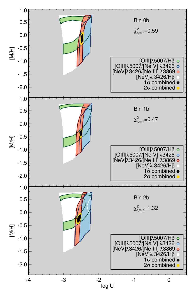
Figure 12.— Plots revealing the allowed parameter space in ionization parameter $U$ and metallicity [M/H] for the emission observed in the bridge (bins 1b and 2b). The grey region in each plot is excluded because these models predict significant emission from lines that are not detected at that level (e.g., Fe VII, O VI, O II). The colored areas in each figure represent the $1\sigma$ $\chi^{2}$ contours for a series of line ratios as labelled. The black and yellow contours correspond respectively to the 1$\sigma$ and 2$\sigma$ confidence intervals for the combined $\chi^{2}$ contours of all 4 line ratios. Note that the entire region which is not grey is allowed at $1\sigma$ confidence for the [Ne V]$\lambda 3462$/H$\beta$ ratio for bins 0b and 1b. Table 4 lists the best fit values.

6.2.3 Quasar Ionization Modelling & Bridge Metallicity

In the previous sections we ruled out shocks and stellar photoionization as the source of ionization for the bridge material. We also inferred, from investigation of the BPT diagram, that the line ratios were likely the result of photoionization by a quasar. In this section, we test this hypothesis by comparing our observations with photoionization models.

Emission line ratios can inform one about the physical conditions of a photoionized gas as well as the properties of the incident ionizing radiation. We utilize cloudy version 08.00 photoionization simulations (Ferland et al., 1998) to determine if photoionization by a quasar’s radiation field can reproduce our observed line ratios and then we infer physical conditions from these ratios.

Our observations include a variety of line ratios for this purpose. We focus on lines with relatively high signal to noise and ratios that depend sensitively on ionization state and metallicity: [O III]$\lambda$5007/H$\beta$, [O III]$\lambda$5007/[Ne V]$\lambda$3426, [Ne V]$\lambda$3426/H$\beta$, and [Ne V]$\lambda$3426/[Ne III]$\lambda$3869. By studying line ratios instead of absolute luminosities, the results are insenstiive to the detailed geometry of the system.

Our models are plane-parallel slabs of gas illuminated by an ionizing spectrum. We parameterize the shape of the ionizing continuum as a power law with a spectral index of $\alpha=-0.4$ from 0.01 to 20 Rydberg (consistent with results from modelling the QSO SED as described in Paper II).The results are not very sensitive to changes in the spectral range the power law covers. We included the appropriate CMB as well as cosmic rays, but these sources of ionization have little consequence for our calculations. We ran models with metallicities of $-2.5<$[Fe/H]$<1.0$ . We note that our implementation of metallicity is just a scaling of all elements equally relative to solar and hence [Fe/H] can be interpreted as a generic [M/H], [O/H], or any [X/H]. We varied the strength of the ionizing radiation by varying the ionization parameter $U$ which is defined as the ratio of the ionizing photon density to hydrogen density:

$$\log U=\log\left(\frac{S}{4\pi r^{2}cn}\right)$$ (13)

where $r$ is the distance from the ionizing source, $n$ is the number density of the gas, and $S$ is the ionizing photon luminosity of the source. We set the hydrogen density to be $10\,\mbox{cm}^{-3}$ (however the particular value was not relevant because we varied the ionization parameter $U$, and optically thin gas is homologous in $U$). We chose the gas stopping column density to be such that the gas was optically thin ($N_{HI}=16.8$). We have adopted the optically thin regime because we see ionization extending throughout the entire 38 $h_{72}^{-1}\,\rm kpc$ extent of the bridge. Optically thick models would need to be clumpy and only partially covering the source. We discuss futher the implications of clumpy models in Paper II.

Table 4Measured & Derived Properties

Property	Estimated Value	Section
Merger
$z_{QSO}$	$0.369\pm 0.001$	3.2
observed $\Delta v$	$30\pm 30$ km/s	4.3
Projected Distance	38 $h_{72}^{-1}$ kpc	3.3
Merger Stage	Between First and Second Passage	7
Quasar
$M_{BH}$	$10^{8.7}M_{\odot}$	5.1; Shen et al. (2008)
$L_{Bol}$	$10^{45.7}$ erg/s	5.1; Shen et al. (2008)
Eddington Ratio	0.07	5.1; Shen et al. (2008)
Host DM Mass	$>8.8\times 10^{11}M_{\odot}$	5.1
Companion Galaxy
Concentration	$>$2.61	3.1
SFR4	$1.61\pm 0.03M_{\odot}$ yr-1	5.2.1
Assuming SFR3=SFR${}_{4};SFR$	$3.22\pm 0.06M_{\odot}$ yr-1	5.2.1
Assuming R-band Light traces SF; SFR	$8.05\pm 0.15M_{\odot}$ yr-1	5.2.1
$12+\log(\mbox{O}/\mbox{H})$	$8.64\pm 0.01\pm 0.2$	5.2.1
$M_{DM}$	$>2.1\times 10^{11}M_{\odot}$	5.2.2
$M_{\star}$	$1.9\times 10^{10}M_{\odot}$	5.2.2
SHAM $M_{DM}$	$6\times 10^{11}M_{\odot}$	5.2.2
SSP Age	300-800 Myr	5.2.3
Burst Mass Fraction	1-100%	5.2.3
Bridge
Kinematics	See Fig. 8	4.3
$\mathcal{D}$	$<10.2h_{72}^{-1}$ kpc	3.3
$n_{H}$	$\approx f^{-1/2}\left(\frac{\mathcal{D}}{1\rm kpc}\right)^{-1}\mbox{ cm}^{-3}$	6.1
$N_{H,\perp}$	$\approx f^{1/2}\ 10^{21}\mbox{ cm}^{-2}$	6.1
$M_{H}$	$\approx 10^{8}\ f^{1/2}\left(\frac{\mathcal{D}}{1\rm kpc}\right)M_{\odot}$	6.1
Source of Ionization	QSO Photoionization	6.2
Bin 0b $\log U$	$-2.48_{-0.02}^{+0.03}$	6.2.3
Bin 0b [M/H]	$-0.13_{-0.16}^{+0.16}$	6.2.3
Bin 0b $\chi^{2}_{r}$	0.59	6.2.3
Bin 1b $\log U$	$-2.50_{-0.02}^{+0.03}$	6.2.3
Bin 1b [M/H]	$-0.36_{-0.12}^{+0.12}$	6.2.3
Bin 1b $\chi^{2}_{r}$	0.47	6.2.3
Bin 2b $\log U$	$-2.56^{+0.05}_{-0.05}$	6.2.3
Bin 2b [M/H]	$-0.23^{+0.14}_{-0.16}$	6.2.3
Bin 2b $\chi^{2}_{r}$	1.32	6.2.3

We compared our line ratios to the models using a $\chi^{2}$ statistic which requires careful estimation of the errors on those line ratios. We refined our error estimates by including an additional 10 percent error on lines if they are part of a line ratio that spanned different cameras to account for relative fluxing issues. The models do not take into account any dust that may be a result of an intervening screen of material between the region of emission and the observer. To characterize the error associated with this, we turned to our measured line ratios. Specifically, we characterized our errors from reddening through 1000 Monte Carlo realizations of the observed H$\alpha$/H$\beta$ ratio. We adopted the observed ratio with a normally distributed error to determine the intrinsic reddening and then corrected the line ratios. This created 1000 “actual” line ratios whose standard deviation we used to estimate the error due to intrinsic reddening. The log relative errors on ([O III]$\lambda$5007/H$\beta$, [Ne V]$\lambda$3426/[Ne III]$\lambda$3869, [Ne V]$\lambda$3426/H$\beta$, [O III]$\lambda$5007/[Ne V]$\lambda$3426) were (-1.4,-0.9,-0.12,-0.62) for 0b, (-1.8,-1.5,-0.8,-0.7) for bin 1b, and (-4.1,-3.7,-3.0,-3.05) for bin 2b. The relative errors are much lower for bin 2b, because the observation places it slightly below the theoretical value.

We first ruled out any models that predicted detectable fluxes (30% of the luminosity of [O III]$\lambda 5007$) for high ionization lines (e.g. Fe VII 6087, O VI 5291, etc.) or low ionization lines (e.g. O II) which are not detected at that level in the bridge. This rules out low and high ionization paramters ($\log U<-3;\log U>-2$) where [OIII] 5007 is predicted to be weak relative to these lines. This resulted in the excluded region denoted grey in Fig. 12. With well-characterized errors and the suite of models in hand, we next constructed $\chi^{2}$ contour surfaces as a function of both $U$ and [M/H]. Here we see that the [Ne V]$\lambda$3426/[Ne III]$\lambda$3869 constrains $\log U$ to a narrow region. We see that our best constraint on [M/H] comes from [O III]$\lambda$5007/H$\beta$. The intersection of these two allow a that region is double valued. The overall $\chi^{2}$ and the [O III]$\lambda$5007/[Ne V] ratio, however, break this degeneracy. Due to lower signal-to-noise, the [Ne V]$\lambda$3426/H$\beta$ ratio offers little additional constraint. The combined constraint lies in the same region for all three bins and allows us to estimate both [M/H] and $\log U$ with relatively high precision (summarized in Table 4).

The best fit models for bin 0b, bin 1b and bin 2b had $\chi^{2}_{r}$ of 0.59, 0.47 and 1.32 respectively and predict [O III]$\lambda$4363/ [O III]$\lambda$5007=0.03 which is well below our detection limit. Therefore these models reproduce the observed [Ne V] emission at a low electron temperature ($T_{e}\sim 1.8\times 10^{4}$ K). There are additional systematic errors associated with the simple geometry in cloudy, the presumption of equilibrium, and uncertainty in the ionization spectral shape (e.g. variations in the spectral index of the power law $\alpha$). We characterize a systematic error based on variations of the power law index of a few tenths to produce an additional uncertainty on $\log U$ of $\approx 0.05$ dex and on [M/H] of $\approx 0.06$ dex.

Lastly, we need to determine if the derived values for the material make physical sense. Given that a quasar can output $10^{56}$ ionizing photons per second (Tadhunter, 1996) and the bridge is approximately 20 kpc away, this yields a possible $U$ parameter of $\log U=-1.16-\log n$. Noting that the QSO could always be partially obscured or non-isotropic, the quasar is a feasible source for any density greater than $\log n\approx-1.5\mbox{ cm}^{-3}$. We also point out that our estimates for $U$ do not appear to fall off as $1/r^{2}$ from the quasar. In Paper II, we discuss various possible interpretations of this observation.

Table 5Comparison with Theory

Theoretical Prediction	Reference	Observation	Consistent?
Galaxy internal parameters	Mihos & Hernquist (1996)	One galaxy is a quasar,	Y
determine their evolution in a merger		one has no AGN activity
First passage inspires a starburst	Mihos & Hernquist (1996)	Starburst spectrum observed	Y
		after first passage, before second
Mergers may lead to quasars	Hopkins et al. (2008a)	One galaxy observed as a quasar	Y
This quasar phase typically	Hopkins et al. (2008a)	Merger between first	?
occurs during final coalescence		and second passage
Starburst & tidal effects may	Stockton (1982)	Imaging is mildly concentrated,	?
lead to a concentrated morphology		but inconclusive due to
		insufficient spatial resolution
2 Gyr timescale between first	Lotz et al. (2010b)	$t=300-800$ Myr after first	Y
and second passage		passage, before second passage
Kinematics near apogee have	Chilingarian et al. (2010)	$\Delta v=30\pm 30$ km/s	Y
small relative velocity	i.e. GalMer

7. Discussion

In this section, we first synthesize the primary results of the preceeding sections (summarized in Table 4) and then consider the implications for research in galaxy mergers and evolution.

The J2049$-$0012 system is a pair of interacting galaxies. Its hallmark is an emission-line bridge that connects the two galaxies, observed in recombination and forbidden line-emission. The observation of the bridge requires that the galaxies (now with a projected separation of 38 $h_{72}^{-1}\,\rm kpc$) have had at least one tidal interaction. One of the galaxies is currently in a quasar phase ($L_{Bol}=10^{45.7}$ erg/s) and its ionizing radiation has photoionized the gas in the bridge, producing the observed line-emission. Using a simplistic volume model for the gas in the bridge, we constrained its surface and volume densities and provided an estimate of the total gas mass ($\sim 10^{8}M_{\odot}$).

Despite its neighbor undergoing a violent quasar phase, the companion galaxy shows no detectable AGN activity. Its photometry and spectrum place it within or near the galaxy ‘green valley’ and also suggest a declining starburst stellar population (with burst age of $300-800$ Myr). The companion galaxy has a current SFR of $\sim 6\ M_{\odot}\mbox{ yr}^{-1}$ and a gas-phase metallicity consistent with solar. This metallicity is higher by $\approx 0.4$ dex than our estimate for the bridge, as derived from Cloudy photoionization modelling.

We made several mass estimates and constraints for both the quasar host and companion galaxy. In the context of galaxy mergers, the mass-ratio of the galaxies is a fundamental quantity because it strongly influences the dynamics of the interaction. Our system has several pieces of evidence which suggest it has a mass ratio of $\approx$ 1:4 and perhaps somewhat smaller. Firstly, examination of the dynamical measurements shows that the companion galaxy’s rotation curve flattens at a velocity of 110  ${\rm km~{}s^{-1}}$ while the QSO host’s extends to a velocity of 200 ${\rm km~{}s^{-1}}$ and shows no signs of flattening. Unless the companion galaxy is seen relatively close to face on, it likely has a significantly lower DM mass than the QSO host. Additionally, our estimates for the stellar masses of the two systems is roughly 1:4. For the companion galaxy, we analyzed the SDSS photometry to estimate a stellar mass of $1.9\times 10^{10}M_{\odot}$. For the galaxy hosting the quasar, we cannot directly measure the stellar light but instead estimate its stellar mass using standard SMBH-host relations. Taking the estimated SMBH mass of $10^{8.7}M_{\odot}$ (Shen et al., 2008) and the Magorrian et al. (1998) relation $M_{BH}\sim 0.006\ M_{host,\star}$, we estimate $8\times 10^{10}M_{\odot}$ for the stellar mass of the bulge component. This gives a stellar mass ratio of $\approx$1:4. If the quasar host galaxy has a stellar mass in a disk component then this ratio shrinks even smaller. This result also hinges on whether the black hole currently lies on the Magorrian relation. We conclude, therefore, that the system has a mass ratio of approximately 1:4 with an uncertainty on the order of a factor of 2. Therefore, the event most likely either just satisfies the major-merger (1:4) definition or lies somewhat below the canonical threshold.

Our observational analysis of the J2049$-$0012 system provides a comprehensive and quantitative description of an interacting pair of galaxies at $z\sim 0.4$. In turn, it affords the opportunity to directly test the standard paradigm for galaxy mergers as modeled by numerical simulations (e.g. Chilingarian et al., 2010; Cox et al., 2006). The current theoretical understanding of galaxy interactions is that galaxy mergers with mass ratios larger than $\approx$ 1:10 generally follow a basic sequence of events with two possible phases of elevated star formation and AGN activity: one right after first passage and the other during final coalescence. The absolute and relative strengths of these two phases depends on the galaxy morphology (e.g. whether the galaxies have gas, the presence of a bulge) and details of the star-formation prescription. In such a paradigm, the combination of the detection of a tidal bridge and the current projected separation of $38h_{72}^{-1}$ kpc place a strong constraint on the merger stage. Numerical simulations of major mergers with a variety of orbits (e.g. Chilingarian et al., 2010) show that after first passage the galaxies move to a distance of approximately 100 kpc where they reach their point of maximal separation (first apogee). Subsequent passages and separations do not achieve separations as large as 38 kpc. This result is nearly independent of gas fraction (Lotz et al., 2010a) and mass ratio as long as the mass ratio is larger than 1:9 (Lotz et al., 2010b). We conclude, therefore, that the J2049$-$0012 merger is after first passage (the bridge requires at least one tidal interaction) and before second passage.

As described above, the current paradigm predicts that gas-rich galaxies will undergo a burst of star-formation that initiates during or just after first passage (e.g. Mihos & Hernquist, 1996). This is also the only time aside from coalescence where gas inflow is predicted to be sufficiently strong to inspire strong AGN activity (Springel et al., 2005a; Hopkins et al., 2008a). Regarding the J2049$-$0012 merger, we identify examples of each: one galaxy hosts a bright quasar and the companion galaxy shows signatures of a starburst stellar population (Figure 10). Consistent with theory of interactions causing tidal stripping and strong gaseous inflows which lead to large central star bursts, the companion galaxy is observed to be consistent with being centrally concentrated (we measure a concentration of at least 2.61, limited by the image’s spatial resolution). Such compact companions to quasars have been observed around other more nearby QSOs (Canalizo & Stockton, 2001; Stockton, 1982). With standard stellar population modeling, we found the burst occurred $300-800$ Myr ago. This timescale is significantly shorter than the predicted period between first and second passage for galaxies with our allowed range of mass ratios for standard orbits ($\approx 2$ Gyr; e.g. Lotz et al., 2010b; Chilingarian et al., 2010) .

In merger simulations, the level of enhanced star formation during the first passage starburst is sensitive to the star formation prescription (see Cox et al., 2006). Therefore characterizing this phase may allow greater insights on sub-grid models. To this end, we would like to constrain the observed mass fraction of the burst. Unfortunately, various degeneracies limit us to only constrain the burst to consist of between $1-100\%$ of the stellar mass prior to the merger.

Another test of the merger paradigm combines the timing of the starburst and the observed configuration of the merger. The current projected separation of 38 $h_{72}^{-1}\,\rm kpc$ combined with the timescale of $~{}500$ Myr requires that the galaxies have been moving apart from each other at an average speed of approximately $75$ ${\rm km~{}s^{-1}}$. This is consistent with the observed timescales and distances seen in GalMer merger simulations (Chilingarian et al., 2010). The observed offset in radial velocities of the two galaxies also follows the standard picture. The centers of mass for the two galaxies (as traced by the bright emission lines) are moving at a relative radial velocity of $30\pm 30$${\rm km~{}s^{-1}}$. This is consistent with the system being close to apogee, as predicted for a system with an age of $t\sim 500$ Myr post first passage (e.g. Lotz et al., 2010b).

Lastly, merger simulations also offer robust predictions on the physical characteristics of the tidal bridge. In the following few paragraphs, we discuss how measurements of the bridge properties test the merger paradigm and also present a means for gaining greater understanding into specific mergers.

Firstly, we note that the metallicity of the bridge, which we find to be a few tenths dex lower ($\Delta$[M/H]=$-0.36\pm 0.23$) than the companion galaxy, is consistent with having been tidally stripped from the (presumed) lower metallicity outskirts of that galaxy. This is the standard result of the merger paradigm first studied in detail by Toomre & Toomre (1972b). The outer parts of these extended tidal features arise from the outskirts of galactic disks because the tidal forces are greatest in these regions.

Due to the unique emission line bridge of our system, we are able to measure the gas surface density at a point midway between the two interacting galaxies ($\S$6.1). Wishing to use this measurement to gain more insight on the interacting pair of galaxies, we turn to numerical simulations. As this is not a standard observable and lacks sufficient literature detailing its evolution, we have explored the GalMer database of galaxy mergers to characterize the bridge’s evolution (Chilingarian et al., 2010). Using a suite of 1:1 and 1:10 galaxy merger simulations with a variety of spiral morphologies (1:1 Sa-Sa, Sa-Sb, Sa-Sd, Sb-Sb, Sb-Sd, Sd-Sd ; 1:10 S0-Sa, S0-Sb, S0-Sd ), we measured the gas surface density in the corresponding regions of these galaxy mergers at 64 viewing angles evenly spaced in solid angle at all applicable timesteps (where the galaxies are separated by at least 20 projected kpc and have undergone at least one tidal interaction). The 1:1 mergers have 12 different orbits with each orbit also having 4 different relative orientations of the disks. The 1:10 mergers are limited by the availability of the models to only have 6 orbits with only 1 generic disk orientation each.

We find that for 1:1 mergers, the bridge forms after first passage and that its surface density reduces roughly exponentially with time (approximately $\propto\exp[-t/\tau]$ with $\tau\approx$100 Myr and the normalization correlating with the gas mass of the two galaxies) as the material rains back onto the two separating galaxies. In the vast majority of cases, the gas density falls far below the measured surface density of our bridge before reaching second closest approach. These findings indicate standard merger scenarios of galaxies with high gas fraction can reproduce our observations provided we have caught the system before maximal separation.

For 1:10 mergers we find that the gaseous bridge does not reach sufficiently high surface densities in the bridge for any of the simulations we examined. We do note that in our 1:10 simulations the larger galaxy does not contain any gas (we are limited by availability of simulations), which is likely a poor match to our system. This is unlikely to affect our overall results because in such a high mass ratio merger the contribution of the more massive galaxy to the extended tidal features will be minimal because the tidal force it feels is relatively small. In such a case, the smaller galaxy is much more greatly tidally perturbed, resulting in extended tidal features but at much smaller surface density than observed. If the mass ratio of the J2049$-$0012 system were as small as 1:10, these models would be ruled out.

The kinematics of the bridge further enlighten us about the system (See Fig. 8). The velocity centroids of the bridge as a function of spatial position show that the side of the bridge closer to the companion galaxy has a higher radial velocity than the side closer to the quasar. If the gas is freely flowing towards the centers of mass of the two galaxies, this suggests that the companion galaxy is background to the quasar. This argument is confirmed by an examination of the GalMer merger simulations. The measured velocity dispersion of $~{}50$ km/s indicates an intrinsic velocity dispersion of $~{}40$ km/s after we remove instrumental effects. This is much higher than that found in 21 cm maps of tidal debris around local interacting galaxies which have typical velocity dispersions of $~{}10-20$ km/s (Hibbard & van Gorkom, 1993, 1996). One possible explanation is suggested by the clumpy nature of the emission: portions of the bridge may have become self-gravitating. Such structures are observed in the tidal features of local galaxies and can have large velocity gradients $>40$ km/s (Weilbacher et al., 2003, 2002). These structures are also a prediction of merger simulations (Barnes & Hernquist, 1992). It is possible that one or several of these structures could add to the velocity dispersion. One immediate challenge to this possibility is the lack of obvious star formation associated with the bridge. However, if the bridge is fully ionized, it is possible that the large ionization fraction of the gas has suppressed star formation. This is supported by the recent observational evidence that there is a neutral gas column density threshold ($\log N_{HI}>20.6\mbox{ cm}^{-2}$) for star formation in tidal material (Maybhate et al., 2007). Another possible explanation is that dispersion has been elevated by some sort of turbulence possibly associated with shocks that are thought to occur throughout the course of the merger as a result of the bulk motions of the galaxies.

Given that we observe a bridge of material that we believe to be photoionized by the quasar, one might ask if other tidal material should be observable (i.e. structures associated with extended tidal tails). We have not detected such material, to sensitive limits, in our Keck/LRIS longslit observations. There are several reasons, however, why we may expect the non-detection of other extended emission. Firstly, there may be no tidal tails. Hibbard et al. (2001) present a compilation of H I maps of merging galaxies and find 16 examples of merging galaxy pairs (of 181 total unusual gas morphology examples) with an observed bridge and no tidal tails. Similarly, the GalMer merger simulation database (Chilingarian et al., 2010) has many examples of such systems. Secondly, the tidal tails may simply not have fallen into the longslit of our spectroscopic observations. Finally, the tidal material could have too low density to render it observable; emission is an $n^{2}$ process and a factor of 3 less dense gas results $\sim 10$ times fainter emission. We conclude that the non-detection of additional, tidal material is consistent with the observed bridge and standard merger scenarios. Nevertheless, we are motivated to search for additional emission beyond our longslit observation, e.g. with an IFU spectrometer.

Before concluding, we wish to consider a few issues related to the ‘green valley’ nature of the companion galaxy. We remind the reader that this is a rare and poorly understood phase of galaxy evolution which nevertheless may be critical to understanding the (expected) transition from the blue, star-forming sequence to the ‘red and dead’ sample. The first consideration is to understand why the galaxy appears in this unusual portion of color space. We have found that the peculiar colors are consistent a declining starburst stellar population that would dominate the SED for only another few hundred Myr. The next obvious consideration is whether the galaxy is currently moving toward the blue cloud or red sequence. Unfortunately, any such prediction hinges on bold extrapolation of the future SFH. If we assume that the observed SFR continues indefinitely (i.e. at $\approx 6M_{\odot}$), then we find that the galaxy evolves to becomes slightly bluer ($u-g$ decreasing by 0.1 mag) over approximately 1 Gyr. However if the star formation ceases then the stellar populations will passively evolve to become red after several hundred Myr. If the galaxies are to undergo further interactions with each other, then the star formation history may follow one of the standard tracks towards quenching (see discussion in Faber et al., 2007).

This system may also provide insights on some of the large number of newly discovered double peaked [O III] emitters (Smith et al., 2010). If observed with sufficiently poor spatial resolution, it is possible that the bridge or the companion galaxy’s emission associated with photoionization from the quasar may result in the appearance of a double-peaked [O III] profile separated by approximately 20 km/s resulting from just a single active SMBH. One could imagine that if caught closer in time to a close passage, where the radial velocity difference of the two galaxies would be greater, the velocity difference may be large enough to produce the $\sim 200$ km/s offsets observed in that sample. This explanation is may be the most likely for a subset of their systems (Rosario et al. in prep.).

8. Summary

In summary, we have compiled physical constraints on a galaxy merger at modest redshift which allows for a direct test of the merger paradigm developed by state-of-the-art simulations. Impressively, the merger characteristics are consistent with the standard paradigm for each of the comparisons summarized in Table 5. Our analysis presents a relatively clear-cut example of a quasar being triggered during a first passage interaction. Observational characteristics allow it to be directly compared with simulations to constrain triggering mechanisms.

We have copious amounts of information about the companion galaxy and obvious questions emerge such as: Why is one galaxy in a quasar phase while the other is not? Has the companion galaxy already undergone a quasar phase? Are the black holes in each galaxy now and will they later be on the many black hole-host relations? How does a first passage quasar affect the evolution of a merger vs. one where neither galaxy goes into a quasar phase until final coalescence? Paper II presents the insights that we gain from this system about some of these questions as well as discusses constraints on the quasar’s lifetime and isotropy that we get by examining the effects of its ionizing radiation.

Our work focuses on characterizing the system as well as possible. A summary of our derived properties can be found in Table 4 and a review of our conclusions follows below.

1. We presented a unique interacting quasar/galaxy pair connected by a remarkable 38 $h_{72}^{-1}\,\rm kpc$ bridge of ionized gas visible in emission lines.

2. While one galaxy is in a quasar phase, its companion shows no detectable AGN activity.

3. After ruling out collisional ionization and radiative shocks, we conclude the bridge’s source of ionization to be photoionization by the quasar light.

4. The companion galaxy’s color and spectrum are consistent with a declining starburst stellar population. In this scenario, we date the burst stellar population to be $300-800$ Myr old. This intermediate-age stellar population places the galaxy within the ‘green valley’.

5. We found the companion galaxy to have a SFR of $\sim 6\ M_{\odot}\mbox{ yr}^{-1}$ and to have a have a gas-phase oxygen abundance consistent with solar.

6. The bridge between the two galaxies was characterized to be dependent on a geometric parameter $\mathcal{D}$, which we constrain (see Fig. 5). We found expressions for the volume density, column density along line of sight, and mass of the bridge as a function of this parameter.

7. With cloudy photoionization modeling, we determine the ionization parameter and metallicity in two separate patches of the bridge. The bridge is nearly fully ionized in hydrogen and is primiarly comprised of higher ionization species. The metallicity is consistent with being a few tenths dex smaller than the companion galaxy.

8. The bridge’s velocity dispersion is larger than expected ($\sim 40$km/s), possibly suggesting that some material in the bridge may be self-gravitating or there is some source of turbulence in the bridge.

9. Using the projected separation, we find the merger stage to be between first and second passage. This interpretation is consistent with the observed bridge and the inferred starburst stellar population.

10. Based on dynamical measurements and stellar photometry, we argue the mass ratio is likely $\sim$1:4.

References

- Abazajian et al. (2009) Abazajian, K. N., et al. 2009, ApJS, 182, 543
- Abel & Satyapal (2008) Abel, N. P., & Satyapal, S. 2008, ApJ, 678, 686
- Adelman-McCarthy et al. (2007) Adelman-McCarthy, J. K., et al. 2007, ApJS, 172, 634
- Allen et al. (2008) Allen, M. G., Groves, B. A., Dopita, M. A., Sutherland, R. S., & Kewley, L. J. 2008, ApJS, 178, 20
- Allende Prieto, Lambert, & Asplund (2001) Allende Prieto, C., Lambert, D. L., & Asplund, M. 2001, ApJ, 556, L63
- Arp (1966) Arp, H. 1966, Atlas of peculiar galaxies, ed. Arp, H.
- Asplund et al. (2004) Asplund, M., Grevesse, N., Sauval, A. J., Allende Prieto, C., & Kiselman, D. 2004, A&A, 417, 751
- Baldwin et al. (1981) Baldwin, J. A., Phillips, M. M., & Terlevich, R. 1981, PASP, 93, 5
- Barnes & Hernquist (1992) Barnes, J. E., & Hernquist, L. 1992, Nature, 360, 715
- Bennert et al. (2008) Bennert, N., Canalizo, G., Jungwiert, B., Stockton, A., Schweizer, F., Peng, C. Y., & Lacy, M. 2008, ApJ, 677, 846
- Blanton & Roweis (2007) Blanton, M. R., & Roweis, S. 2007, AJ, 133, 734
- Bohlin (1996) Bohlin, R. C. 1996, AJ, 111, 1743
- Bohlin et al. (2001) Bohlin, R. C., Dickinson, M. E., & Calzetti, D. 2001, AJ, 122, 2118
- Booth & Schaye (2009) Booth, C. M., & Schaye, J. 2009, MNRAS, 398, 53
- Brammer et al. (2009) Brammer, G. B., et al. 2009, ApJ, 706, L173
- Bruzual & Charlot (2003) Bruzual, G., & Charlot, S. 2003, MNRAS, 344, 1000
- Bullock et al. (2001) Bullock, J. S., Kolatt, T. S., Sigad, Y., Somerville, R. S., Kravtsov, A. V., Klypin, A. A., Primack, J. R., & Dekel, A. 2001, MNRAS, 321, 559
- Canalizo & Stockton (2001) Canalizo, G., & Stockton, A. 2001, ApJ, 555, 719
- Cardelli et al. (1989) Cardelli, J. A., Clayton, G. C., & Mathis, J. S. 1989, ApJ, 345, 245
- Chabrier (2003) Chabrier, G. 2003, PASP, 115, 763
- Charlot & Fall (2000) Charlot, S., & Fall, S. M. 2000, ApJ, 539, 718
- Chilingarian et al. (2010) Chilingarian, I. V., Di Matteo, P., Combes, F., Melchior, A.-L., & Semelin, B. 2010, A&A, 518, A61
- Coil et al. (2004) Coil, A. L., Newman, J. A., Kaiser, N., Davis, M., Ma, C., Kocevski, D. D., & Koo, D. C. 2004, ApJ, 617, 765
- Conroy & Wechsler (2009) Conroy, C., & Wechsler, R. H. 2009, ApJ, 696, 620
- Conselice (2003) Conselice, C. J. 2003, ApJS, 147, 1
- Cox et al. (2006) Cox, T. J., Jonsson, P., Primack, J. R., & Somerville, R. S. 2006, MNRAS, 373, 1013
- Croom et al. (2009) Croom, S. M., et al. 2009, MNRAS, 399, 1755
- Cutri et al. (2003) Cutri, R. M., et al. 2003, 2MASS All Sky Catalog of point sources., ed. Cutri, R. M., Skrutskie, M. F., van Dyk, S., Beichman, C. A., Carpenter, J. M., Chester, T., Cambresy, L., Evans, T., Fowler, J., Gizis, J., Howard, E., Huchra, J., Jarrett, T., Kopan, E. L., Kirkpatrick, J. D., Light, R. M., Marsh, K. A., McCallon, H., Schneider, S., Stiening, R., Sykes, M., Weinberg, M., Wheaton, W. A., Wheelock, S., & Zacarias, N.
- Davis et al. (2003) Davis, M., et al. 2003, in Presented at the Society of Photo-Optical Instrumentation Engineers (SPIE) Conference, Vol. 4834, Society of Photo-Optical Instrumentation Engineers (SPIE) Conference Series, ed. P. Guhathakurta, 161–172
- Davis et al. (2007) Davis, M., et al. 2007, ApJ, 660, L1
- Dekel & Birnboim (2006) Dekel, A., & Birnboim, Y. 2006, MNRAS, 368, 2
- Di Matteo et al. (2007) Di Matteo, P., Combes, F., Melchior, A., & Semelin, B. 2007, A&A, 468, 61
- Dressler & Gunn (1983) Dressler, A., & Gunn, J. E. 1983, ApJ, 270, 7
- Ellisonet al. (2008) Ellison, S. L., Patton, D. R., Simard, L., & McConnachie, A. W. 2008, AJ, 135, 1877
- Faber et al. (2007) Faber, S. M., et al. 2007, ApJ, 665, 265
- Fakhouri et al. (2010) Fakhouri, O., Ma, C., & Boylan-Kolchin, M. 2010, MNRAS, 406, 2267
- Ferland et al. (1998) Ferland, G. J., Korista, K. T., Verner, D. A., Ferguson, J. W., Kingdon, J. B., & Verner, E. M. 1998, PASP, 110, 761
- Ferrarese (2002) Ferrarese, L. 2002, ApJ, 578, 90
- Ferrarese & Merritt (2000) Ferrarese, L., & Merritt, D. 2000, ApJ, 539, L9
- Fontana et al. (2006) Fontana, A., et al. 2006, A&A, 459, 745
- Fu & Stockton (2009) Fu, H., & Stockton, A. 2009, ApJ, 690, 953
- Gebhardt et al. (2000) Gebhardt, K., et al. 2000, ApJ, 539, L13
- Graham et al. (2001) Graham, A. W., Erwin, P., Caon, N., & Trujillo, I. 2001, ApJ, 563, L11
- Green et al. (2010) Green, P. J., Myers, A. D., Barkhouse, W. A., Mulchaey, J. S., Bennert, V. N., Cox, T. J., & Aldcroft, T. L. 2010, ApJ, 710, 1578
- Greene et al. (2009) Greene, J. E., Zakamska, N. L., Liu, X., Barth, A. J., & Ho, L. C. 2009, ApJ, 702, 441
- Hibbard et al. (2001) Hibbard, J. E., van der Hulst, J. M., Barnes, J. E., & Rich, R. M. 2001, AJ, 122, 2969
- Hibbard & van Gorkom (1993) Hibbard, J. E., & van Gorkom, J. H. 1993, in Astronomical Society of the Pacific Conference Series, Vol. 48, The Globular Cluster-Galaxy Connection, ed. G. H. Smith & J. P. Brodie, 619–+
- Hibbard & van Gorkom (1996) Hibbard, J. E., & van Gorkom, J. H. 1996, AJ, 111, 655
- Hibbard et al. (2001) Hibbard, J. E., van Gorkom, J. H., Rupen, M. P., & Schiminovich, D. 2001, Gas and Galaxy Evolution, 240, 657
- Ho (2005) Ho, L. C. 2005, ApJ, 629, 680
- Hopkins et al. (2008a) Hopkins, P. F., Hernquist, L., Cox, T. J., & Kereš, D. 2008a, ApJS, 175, 356
- Hopkins et al. (2008b) —. 2008b, ApJS, 175, 356
- Kauffmann et al. (2003a) Kauffmann, G., et al. 2003a, MNRAS, 341, 54
- Kauffmann et al. (2003b) —. 2003b, MNRAS, 346, 1055
- Kelly et al. (2010) Kelly, B. C., Vestergaard, M., Fan, X., Hopkins, P., Hernquist, L., & Siemiginowska, A. 2010, ApJ, 719, 1315
- Kennicutt (1998) Kennicutt, Jr., R. C. 1998, ARA&A, 36, 189
- Kewley et al. (2001) Kewley, L. J., Dopita, M. A., Sutherland, R. S., Heisler, C. A., & Trevena, J. 2001, ApJ, 556, 121
- Kocevski et al. (2009) Kocevski, D. D., Lubin, L. M., Lemaux, B. C., Gal, R. R., Fassnacht, C. D., Lin, R., & Squires, G. K. 2009, ApJ, 700, 901
- Kong et al. (2006) Kong, M., Wu, X., Wang, R., & Han, J. 2006, Chinese Journal of Astronomy and Astrophysics, 6, 396
- Lotz et al. (2008a) Lotz, J. M., Jonsson, P., Cox, T. J., & Primack, J. R. 2008a, MNRAS, 391, 1137
- Lotz et al. (2010a) —. 2010a, MNRAS, 404, 590
- Lotz et al. (2010b) —. 2010b, MNRAS, 404, 575
- Lotz et al. (2008b) Lotz, J. M., et al. 2008b, ApJ, 672, 177
- Magorrian et al. (1998) Magorrian, J., et al. 1998, AJ, 115, 2285
- Martin et al. (2005) Martin, D. C., et al. 2005, ApJ, 619, L1
- Martin et al. (2007) Martin, D. C., et al. 2007, ApJS, 173, 342
- Martini & Schneider (2003) Martini, P., & Schneider, D. P. 2003, ApJ, 597, L109
- Martini & Weinberg (2001) Martini, P., & Weinberg, D. H. 2001, ApJ, 547, 12
- Matthews & Sandage (1963) Matthews, T. A., & Sandage, A. R. 1963, ApJ, 138, 30
- Maybhate et al. (2007) Maybhate, A., Masiero, J., Hibbard, J. E., Charlton, J. C., Palma, C., Knierman, K. A., & English, J. 2007, MNRAS, 381, 59
- Mihos & Hernquist (1994) Mihos, J. C., & Hernquist, L. 1994, ApJ, 431, L9
- Mihos & Hernquist (1996) —. 1996, ApJ, 464, 641
- Miller & Stone (1993) Miller, J. S., & Stone, R. P. S. 1993, Lick Observatory Technical Reports 66 (Santa Cruz, CA; Lick Observatory)
- Nandra et al. (2007) Nandra, K., et al. 2007, ApJ, 660, L11
- Noeske et al. (2007) Noeske, K. G., et al. 2007, ApJ, 660, L47
- Noeske et al. (2007) Noeske, K. G., et al. 2007, ApJ, 660, L43
- Oke et al. (1995) Oke, J. B., et al. 1995, PASP, 107, 375
- Osterbrock & Ferland (2006) Osterbrock, D. E., & Ferland, G. J. 2006, Astrophysics of gaseous nebulae and active galactic nuclei, ed. Osterbrock, D. E. & Ferland, G. J.
- Oyaizu et al. (2008) Oyaizu, H., Lima, M., Cunha, C. E., Lin, H., Frieman, J., & Sheldon, E. S. 2008, ApJ, 674, 768
- Penston et al. (1990) Penston, M. V., et al. 1990, A&A, 236, 53
- Pettini & Pagel (2004) Pettini, M., & Pagel, B. E. J. 2004, MNRAS, 348, L59
- Quintero et al. (2004) Quintero, A. D., et al. 2004, ApJ, 602, 190
- Reichard et al. (2009) Reichard, T. A., Heckman, T. M., Rudnick, G., Brinchmann, J., Kauffmann, G., & Wild, V. 2009, ApJ, 691, 1005
- Richards et al. (2002) Richards, G. T., Vanden Berk, D. E., Reichard, T. A., Hall, P. B., Schneider, D. P., SubbaRao, M., Thakar, A. R., & York, D. G. 2002, AJ, 124, 1
- Rosario et al. (2010) Rosario, D. J., Shields, G. A., Taylor, G. B., Salviander, S., & Smith, K. L. 2010, ApJ, 716, 131
- Rubin et al. (2010) Rubin, K. H. R., Weiner, B. J., Koo, D. C., Martin, C. L., Prochaska, J. X., Coil, A. L., & Newman, J. A. 2010, ApJ, 719, 1503
- Schawinski et al. (2009) Schawinski, K., Virani, S., Simmons, B., Urry, C. M., Treister, E., Kaviraj, S., & Kushkuley, B. 2009, ApJ, 692, L19
- Schlegel et al. (1998) Schlegel, D. J., Finkbeiner, D. P., & Davis, M. 1998, ApJ, 500, 525
- Shen et al. (2008) Shen, Y., Greene, J. E., Strauss, M. A., Richards, G. T., & Schneider, D. P. 2008, ApJ, 680, 169
- Smith et al. (2010) Smith, K. L., Shields, G. A., Bonning, E. W., McMullen, C. C., Rosario, D. J., & Salviander, S. 2010, ApJ, 716, 866
- Soltan (1982) Soltan, A. 1982, MNRAS, 200, 115
- Springel et al. (2005a) Springel, V., Di Matteo, T., & Hernquist, L. 2005a, MNRAS, 361, 776
- Springel et al. (2005b) Springel, V., et al. 2005b, Nature, 435, 629
- Stockton (1982) Stockton, A. 1982, ApJ, 257, 33
- Stockton & MacKenty (1987) Stockton, A., & MacKenty, J. W. 1987, ApJ, 316, 584
- Sutter & Ricker (2010) Sutter, P. M., & Ricker, P. M. 2010, ArXiv e-prints
- Szentgyorgyi et al. (2000) Szentgyorgyi, A. H., Raymond, J. C., Hester, J. J., & Curiel, S. 2000, ApJ, 529, 279
- Tadhunter (1996) Tadhunter, C. 1996, Optical spectroscopy of Cygnus A: mixed evidence for a hidden quasar, ed. Carilli, C. L. & Harris, D. E., 33–+
- Toomre (1977) Toomre, A. 1977, in Evolution of Galaxies and Stellar Populations, ed. B. M. Tinsley & R. B. Larson, 401–+
- Toomre & Toomre (1972a) Toomre, A., & Toomre, J. 1972a, ApJ, 178, 623
- Toomre & Toomre (1972b) —. 1972b, ApJ, 178, 623
- Trammell et al. (2007) Trammell, G. B., Vanden Berk, D. E., Schneider, D. P., Richards, G. T., Hall, P. B., Anderson, S. F., & Brinkmann, J. 2007, AJ, 133, 1780
- Veilleux & Osterbrock (1987) Veilleux, S., & Osterbrock, D. E. 1987, ApJS, 63, 295
- Vergani et al. (2010) Vergani, D., et al. 2010, A&A, 509, A42+
- Vestergaard & Peterson (2006) Vestergaard, M., & Peterson, B. M. 2006, ApJ, 641, 689
- Villar-Martín et al. (2010) Villar-Martín, M., Tadhunter, C., Pérez, E., Humphrey, A., Martínez-Sansigre, A., González Delgado, R., & Pérez-Torres, M. 2010, MNRAS, L95+
- Wampler et al. (1975) Wampler, E. J., Burbidge, E. M., Baldwin, J. A., & Robinson, L. B. 1975, ApJ, 198, L49
- Weilbacher et al. (2003) Weilbacher, P. M., Duc, P., & Fritze-v. Alvensleben, U. 2003, A&A, 397, 545
- Weilbacher et al. (2002) Weilbacher, P. M., Fritze-v. Alvensleben, U., Duc, P., & Fricke, K. J. 2002, ApJ, 579, L79
- Weniger et al. (2009) Weniger, J., Theis, C., & Harfst, S. 2009, Astronomische Nachrichten, 330, 1019
- Wild et al. (2009) Wild, V., Walcher, C. J., Johansson, P. H., Tresse, L., Charlot, S., Pollo, A., Le Fèvre, O., & de Ravel, L. 2009, MNRAS, 395, 144
- Wilhite et al. (2005) Wilhite, B. C., Vanden Berk, D. E., Kron, R. G., Schneider, D. P., Pereyra, N., Brunner, R. J., Richards, G. T., & Brinkmann, J. V. 2005, ApJ, 633, 638
- Willmer et al. (2006) Willmer, C. N. A., et al. 2006, ApJ, 647, 853
- Woods & Geller (2007) Woods, D. F., & Geller, M. J. 2007, AJ, 134, 527
- Yan et al. (2006) Yan, R., Newman, J. A., Faber, S. M., Konidaris, N., Koo, D., & Davis, M. 2006, ApJ, 648, 281