Cosmic microwave background bispectrum of tensor passive modes induced from primordial magnetic fields

Abstract

If the seed magnetic fields exist in the early Universe, tensor components of their anisotropic stresses are not compensated prior to neutrino decoupling and the tensor metric perturbations generated from them survive passively. Consequently, due to the decay of these metric perturbations after recombination, the so-called integrated Sachs-Wolfe effect, the large-scale fluctuations of CMB radiation are significantly boosted. This kind of CMB anisotropy is called the “tensor passive mode.” Because these fluctuations deviate largely from the Gaussian statistics due to the quadratic dependence on the strength of the Gaussian magnetic field, not only the power spectrum but also the higher-order correlations have reasonable signals. With these motives, we compute the CMB bispectrum induced by this mode. When the magnetic spectrum obeys a nearly scale-invariant shape, we obtain an estimation of a typical value of the normalized reduced bispectrum as $\ell_{1}(\ell_{1}+1)\ell_{3}(\ell_{3}+1)|b_{\ell_{1}\ell_{2}\ell_{3}}|\sim(130-6)\times 10^{-16}(B_{1\rm Mpc}/4.7{\rm nG})^{6}$ depending on the energy scale of the magnetic field production from $10^{14}$GeV to $10^{3}$GeV. Here, $B_{1{\rm Mpc}}$ is the strength of the primordial magnetic field smoothed on $1{\rm Mpc}$. From the above estimation and the current observational constraint on the primordial non-Gaussianity, we get a rough constraint on the magnetic field strength as $B_{1{\rm Mpc}}<2.6-4.4{\rm nG}$.

I Introduction

Cosmological observations have suggested the existence of micro-Gauss strength magnetic fields in galaxies and clusters of galaxies at the present Universe. As their origin, many researchers have discussed the possibility of generating the seed fields in the early Universe (e.g. Martin and Yokoyama (2008); Bamba and Sasaki (2007)). These scenarios have been verified by constraining the strength of the primordial magnetic fields (PMFs) through the effect on CMB fluctuations.

Conventional studies have provided upper bounds on PMFs with the two point correlations (power spectra) of the CMB temperature and polarization anisotropies Paoletti and Finelli (2010); Shaw and Lewis (2010a). On the other hand, taking into account the CMB three-point correlations (bispectra), which have a nonzero value because the CMB fluctuations are sourced from the quadratic (non-Gaussian) terms of the stochastic (Gaussian) PMFs, some new consequences have been obtained. In Refs. Seshadri and Subramanian (2009); Caprini et al. (2009); Trivedi et al. (2010), the authors evaluated the contribution of the scalar modes at large scale with several approximations, such as the Sachs-Wolfe limit, and roughly estimated the upper limit on the PMF strength. In our previous papers Shiraishi et al. (2010a, 2011a), we computed the effect of the vector modes without neglecting the complicated angular dependence, and obtained tighter bounds due to the dominant contribution at small scale induced by the Doppler and the integrated Sachs-Wolfe (ISW) effects Mack et al. (2002); Kahniashvili and Lavrelashvili (2010). However, if the gravitational waves are generated from the PMF anisotropic stresses uncompensated prior to neutrino decoupling, these superhorizon modes survive passively and the decay of their modes after recombination amplifies the CMB anisotropies through the ISW effect Lewis (2004). This type of fluctuation is called the “tensor passive mode” and it is expected that the CMB bispectrum of this mode has the most dominant signal at large scales, as inferred from the power spectrum Shaw and Lewis (2010b). Therefore, in this paper, we investigate the exact CMB bispectrum of tensor passive modes induced from PMFs and place a new constraint on the strength of PMFs. In the calculation, because there are complicated angular integrals as there are in the vector mode case, we apply our computation approach, as discussed in Ref. Shiraishi et al. (2011a).

This paper is organized as follows. In the next section, we formulate the CMB bispectrum of tensor passive modes induced from PMFs. In Sec. III, we show our result for the CMB bispectrum and the limit on the strength of PMFs, and give a discussion.

II Formulation of tensor bispectrum induced from PMFs

Let us consider the stochastic PMFs $B^{b}({\bf x},\tau)$ on the Friedmann-Robertson-Walker and small perturbative metric as

$$ds^{2}=a(\tau)^{2}[-d\tau^{2}+2h_{0b}d\tau dx^{b}+(\delta_{bc}+h_{bc})dx^{b}dx^{c}]~{}.$$ (1)

Here $a$ is a scale factor and $\tau$ is a conformal time. In this space-time, the PMF evolves as $B^{b}({\bf x},\tau)=B^{b}({\bf x})/a^{2}$. Then the spatial components of the PMF’s energy momentum tensors are given by

$$\begin{split}T^{b}_{~{}c}&=\frac{1}{4\pi a^{4}}\left[\frac{B^{2}({\bf x})}{2}\delta^{b}_{~{}c}-B^{b}({\bf x})B_{c}({\bf x})\right]\\ &\equiv\rho_{\gamma}\left(\Delta_{B}\delta^{b}_{~{}c}+\Pi^{b}_{Bc}\right)~{},\end{split}$$ (2)

where $B^{2}=B^{b}B_{b}$ and we use the photon energy density $\rho_{\gamma}(\propto a^{-4})$ for normalization. In the following discussion, the index is lowered by $\delta_{bc}$, and the summation is implied for repeated indices.

II.1 Bispectrum of the tensor anisotropic stress fluctuations

The Fourier component of $\Pi_{Bab}$ is given by the convolution of the PMFs as

$$\Pi_{Bab}({\bf k})=-\frac{1}{4\pi\rho_{\gamma,0}}\int\frac{d^{3}{\bf k}^{\prime}}{(2\pi)^{3}}B_{a}({\bf k}^{\prime})B_{b}({\bf k}-{\bf k}^{\prime})~{},$$ (3)

where $\rho_{\gamma,0}\equiv\rho_{\gamma}a^{4}$ denotes the present energy density of photons. If $B^{a}({\bf x})$ obeys the Gaussian statistics, the power spectrum of the PMFs $P_{B}(k)$ is defined by

$$\Braket{B_{a}({\bf k})B_{b}({\bf p})}=(2\pi)^{3}{P_{B}(k)\over 2}P_{ab}(\hat{\bf k})\delta({\bf k}+{\bf p})~{},$$ (4)

with a projection tensor

$$P_{ab}(\hat{\bf k})\equiv\sum_{\sigma=\pm 1}\epsilon^{(\sigma)}_{a}\epsilon^{(-\sigma)}_{b}=\delta_{ab}-\hat{k}_{a}\hat{k}_{b}~{},$$ (5)

which comes from the divergenceless of the PMF. Here $\hat{\bf k}$ denotes a unit vector, $\epsilon_{a}^{(\pm 1)}$ is a normalized divergenceless polarization vector satisfying the orthogonal condition, $\hat{k}^{a}\epsilon_{a}^{(\pm 1)}=0$, and $\sigma(=\pm 1)$ expresses the helicity of the polarization vector. In general, the magnetic power spectrum should contain an asymmetric helical term Caprini et al. (2004); Kahniashvili and Ratra (2005); Pogosian et al. (2002). However, we assume the magnetic fields are isotropic and homogeneous, for simplicity; hence, this effect is neglected in Eq. (4). Because the production mechanism of PMFs remains to be done, we use a simple power-law form as the power spectrum:

$$P_{B}(k)={(2\pi)^{n_{B}+5}\over\Gamma(n_{B}/2+3/2)k_{1{\rm Mpc}}^{3}}B_{1{\rm Mpc}}^{2}\left({k\over k_{1{\rm Mpc}}}\right)^{n_{B}}~{},$$ (6)

where $B_{1{\rm Mpc}}$ denotes the magnetic field strength smoothed on a scale $1{\rm Mpc}$, $k_{\rm 1Mpc}\equiv 2\pi{\rm Mpc}^{-1}$, and $n_{B}$ is a spectral index.

With a transverse and traceless polarization tensor Shiraishi et al. (2011b), $e_{ab}^{({\pm 2})}\equiv\sqrt{2}\epsilon_{a}^{(\pm 1)}\epsilon_{b}^{(\pm 1)}$, the anisotropic stress fluctuation is decomposed into two helicity states of the tensor mode as

$$\Pi_{Bab}({\bf k})=\sum_{\lambda=\pm 2}\Pi_{Bt}^{({\lambda})}({\bf k})e_{ab}^{({\lambda})}(\hat{\bf k})~{},$$ (7)

which is inversely converted into

$$\Pi_{Bt}^{({\pm 2})}({\bf k})=\frac{1}{2}e_{ab}^{({\mp 2})}(\hat{\bf k})\Pi_{Bab}({\bf k})~{}.$$ (8)

From the above equations, the bispectrum of $\Pi_{Bt}^{(\pm 2)}$ is symmetrically formed as

$$\Braket{\prod_{n=1}^{3}\Pi_{Bt}^{(\lambda_{n})}({\bf k_{n}})} = \left(-16\pi\rho_{\gamma,0}\right)^{-3}\left[\prod_{n=1}^{3}\int d^{3}{\bf k_{n}^{\prime}}P_{B}(k^{\prime}_{n})\right]\delta({\bf k_{1}}-{\bf k_{1}^{\prime}}+{\bf k_{3}^{\prime}})\delta({\bf k_{2}}-{\bf k_{2}^{\prime}}+{\bf k_{1}^{\prime}})\delta({\bf k_{3}}-{\bf k_{3}^{\prime}}+{\bf k_{2}^{\prime}})$$ (9)

$$\times e^{(-\lambda_{1})}_{ab}(\hat{\bf k_{1}})e^{(-\lambda_{2})}_{cd}(\hat{\bf k_{2}})e^{(-\lambda_{3})}_{ef}(\hat{\bf k_{3}})[P_{ad}(\hat{\bf k_{1}^{\prime}})P_{be}(\hat{\bf k_{3}^{\prime}})P_{cf}(\hat{\bf k_{2}^{\prime}})+\{a\leftrightarrow b\ {\rm or}\ c\leftrightarrow d\ {\rm or}\ e\leftrightarrow f\}],$$

where $\lambda$ means two helicities: $\lambda_{1},\lambda_{2},\lambda_{3}=\pm 2$, and the curly brackets denote the symmetric 7 terms under the permutations of indices: $a\leftrightarrow b$, $c\leftrightarrow d$, or $e\leftrightarrow f$. Because the anisotropic stress fluctuation depends quadratically on the Gaussian magnetic fields as shown in Eq. (3), the statistics of their tensor modes given by (8) is highly non-Gaussian. Hence, the bispectrum of Eq. (9) also has a nonzero value and induces the finite CMB bispectrum.

II.2 CMB temperature bispectrum of tensor passive modes

As is well known, the gravitational potential of tensor modes can be generated from anisotropic stresses via the Einstein equation. If PMFs exist, the anisotropic stresses, as mentioned in the previous subsection, also behave as a source. In general, after neutrino decoupling, the anisotropic stresses of PMFs vanish via the compensation of those of neutrinos. However, prior to this epoch, there is no compensation process due to the absence of the neutrino anisotropic stresses. Hence, from the Einstein equation, we find the evolution equation of the tensor-mode metric perturbations as

$${h^{(\pm 2)}}^{\prime\prime}({\bf k},\tau)+2\frac{a^{\prime}}{a}{h^{(\pm 2)}}^{\prime}({\bf k},\tau)+k^{2}h^{(\pm 2)}({\bf k},\tau)\approx\left\{\begin{array}[]{ll}16\pi Ga^{2}\rho_{\gamma}\Pi^{(\pm 2)}_{Bt}({\bf k})&(\tau_{B}\lesssim\tau\lesssim\tau_{\nu})\\ 0&(\tau\gtrsim\tau_{\nu})\end{array}\right.~{},$$ (12)

where $\tau_{\nu}$ and $\tau_{B}$ are the conformal times at neutrino decoupling and the generation of the PMF, respectively, and ^′ denotes a derivative of conformal time. Here $h^{(\pm 2)}$ is given by

$$h^{({\pm 2})}({\bf k},\tau)=\frac{1}{2}e_{ab}^{({\mp 2})}(\hat{\bf k})h_{ab}({\bf k},\tau)~{}.$$ (13)

From Eq. (12), we find a superhorizon solution of the tensor metric perturbation as Lewis (2004); Shaw and Lewis (2010b)

$$h^{(\pm 2)}({\bf k})\approx h^{(\pm 2)}({\bf k},\tau_{\nu})\approx 6R_{\gamma}\ln\left(\frac{\tau_{\nu}}{\tau_{B}}\right)\Pi_{Bt}^{(\pm 2)}({\bf k})~{},$$ (14)

where $R_{\gamma}\sim 0.6$ is the ratio by the energy density of photons to all relativistic particles for $\tau<\tau_{\nu}$.

The CMB temperature fluctuation is expanded into spherical harmonics as ${\Delta T(\hat{\bf n})\over T}=\sum_{\ell m}a_{\ell m}Y_{\ell m}(\hat{\bf n})$. The $a_{\ell m}$ sourced from the initial tensor perturbations (14) can be expressed as Shiraishi et al. (2011b)

$$a_{\ell m} = (-i)^{\ell}\int{k^{2}dk\over 2\pi^{2}}\mathcal{T}_{\ell}(k)\sum\limits_{\lambda=\pm 2}h^{(\lambda)}_{\ell m}(k)~{},$$ (15)

$$h_{\ell m}^{({\pm 2})}(k) \equiv \int d^{2}\hat{\bf k}h^{({\pm 2})}({\bf k}){}_{\mp 2}Y^{*}_{\ell m}(\hat{\bf k})~{}.$$ (16)

where $\mathcal{T}_{\ell}(k)$ denotes the transfer function of tensor modes. Because the solution of the magnetic passive mode (14), if any, would dominate the tensor-mode perturbation, the evolution of tensor modes after their creation is almost identical to the standard cosmological one without anisotropic stress sources. Therefore, we can use the standard cosmological tensor-mode transfer function Zaldarriaga and Seljak (1997); Weinberg (2008); Shiraishi et al. (2010b).

The CMB angle-averaged bispectrum is given by

$$B_{\ell_{1}\ell_{2}\ell_{3}} = \sum_{m_{1}m_{2}m_{3}}\left(\begin{array}[]{ccc}\ell_{1}&\ell_{2}&\ell_{3}\\ m_{1}&m_{2}&m_{3}\\ \end{array}\right)\Braket{\prod_{n=1}^{3}a_{\ell_{n}m_{n}}},$$ (19)

where the bracket denotes the Wigner-$3j$ symbol.

In order to calculate the bispectrum of $a_{\ell m}$ given by Eq. (15), we rewrite all angular dependencies in Eq. (9) in terms of the spin-weighted spherical harmonics with the notation as Shiraishi et al. (2011b)

$$\begin{split}\epsilon^{(\pm 1)}_{a}(\hat{\bf r})&=\epsilon^{(\mp 1)*}_{a}(\hat{\bf r})=\mp\sum_{m}\alpha^{m}_{a}{}_{\pm 1}Y_{1m}(\hat{\bf r})~{},\\ \alpha^{m}_{a}\alpha^{m^{\prime}}_{a}&=\frac{4\pi}{3}(-1)^{m}\delta_{m,-m^{\prime}}~{}.\end{split}$$ (20)

We then express the angular integrals of the spin spherical harmonics with the Wigner-$3j$ symbols, and sum up these Wigner-$3j$ symbols over the azimuthal quantum numbers in the same manner as in Ref. Shiraishi et al. (2011a). Then, we obtain the final form of the bispectrum as

$$\begin{split}B_{\ell_{1}\ell_{2}\ell_{3}}&=(-4\pi\rho_{\gamma,0})^{-3}\left[\prod\limits^{3}_{n=1}(-i)^{\ell_{n}}\int{k_{n}^{2}dk_{n}\over 2\pi^{2}}\mathcal{T}_{\ell_{n}}(k_{n})\sum\limits_{\lambda_{n}=\pm 2}\int_{0}^{k_{D}}k_{n}^{\prime 2}dk_{n}^{\prime}P_{B}(k_{n}^{\prime})\right]\\ &\quad\times\sum_{LL^{\prime}L^{\prime\prime}}\sum_{S,S^{\prime},S^{\prime\prime}=\pm 1}\left\{\begin{array}[]{ccc}\ell_{1}&\ell_{2}&\ell_{3}\\ L^{\prime}&L^{\prime\prime}&L\end{array}\right\}f^{S^{\prime\prime}S\lambda_{1}}_{L^{\prime\prime}L\ell_{1}}(k_{3}^{\prime},k_{1}^{\prime},k_{1})f^{SS^{\prime}\lambda_{2}}_{LL^{\prime}\ell_{2}}(k_{1}^{\prime},k_{2}^{\prime},k_{2})f^{S^{\prime}S^{\prime\prime}\lambda_{3}}_{L^{\prime}L^{\prime\prime}\ell_{3}}(k_{2}^{\prime},k_{3}^{\prime},k_{3}),\\ f^{S^{\prime\prime}S\lambda}_{L^{\prime\prime}L\ell}(r_{3},r_{2},r_{1})&\equiv-4(8\pi)^{3/2}R_{\gamma}\ln\left(\tau_{\nu}\over\tau_{B}\right)\sum_{L_{1}L_{2}L_{3}}\int_{0}^{\infty}y^{2}dyj_{L_{3}}(r_{3}y)j_{L_{2}}(r_{2}y)j_{L_{1}}(r_{1}y)\\ &\quad\times(-1)^{\ell+L_{2}+L_{3}}(-1)^{(L_{1}+L_{2}+L_{3})/2}I^{0\ 0\ 0}_{L_{1}L_{2}L_{3}}I^{0S^{\prime\prime}-S^{\prime\prime}}_{L_{3}1L^{\prime\prime}}I^{0S-S}_{L_{2}1L}I_{L_{1}\ell 2}^{0\lambda-\lambda}\left\{\begin{array}[]{ccc}L^{\prime\prime}&L&\ell\\ L_{3}&L_{2}&L_{1}\\ 1&1&2\end{array}\right\}~{},\end{split}$$ (21)

where $j_{l}(x)$ is the spherical Bessel function, $k_{D}$ is the Alfvén-wave damping length scale, the $2\times 3$ and $3\times 3$ matrices in the curly brackets denote the Wigner-$6j$ and $9j$ symbols, respectively, and

$$I^{s_{1}s_{2}s_{3}}_{l_{1}l_{2}l_{3}}\equiv\sqrt{\frac{(2l_{1}+1)(2l_{2}+1)(2l_{3}+1)}{4\pi}}\left(\begin{array}[]{ccc}l_{1}&l_{2}&l_{3}\\ s_{1}&s_{2}&s_{3}\end{array}\right)~{}.$$ (24)

As shown in Eq. (21), the bispectrum depends on $\tau_{B}$. Although the production mechanism of PMFs is unclear and still being discussed, we assume that PMFs arise sometime between the energy scale of any grand unification theory and the electroweak transition. Hence, in the computation of the CMB bispectrum, we consider two corresponding values: $\tau_{\nu}/\tau_{B}\sim 10^{17},10^{6}$. This leads to a factor of $23$ difference in the amplitude of the CMB bispectrum due to the logarithmic dependence on $\tau_{\nu}/\tau_{B}$. Therefore, due to the sextuplicate dependence of the CMB bispectrum on the magnetic strength, there is a model-dependent factor $23^{1/6}\simeq 1.7$ in bounds with the PMF strength.

III Numerical results and discussion

Following the final expression (21), we compute the CMB temperature bispectrum of tensor passive modes numerically .

In Fig. 1, we describe the reduced bispectra of temperature fluctuations induced by the PMFs defined as Komatsu and Spergel (2001) $b_{\ell_{1}\ell_{2}\ell_{3}}\equiv(I^{0\ 0\ 0}_{\ell_{1}\ell_{2}\ell_{3}})^{-1}B_{\ell_{1}\ell_{2}\ell_{3}}$, for $\ell_{1}=\ell_{2}=\ell_{3}$. From the red solid lines, we can find that the enhancement at $\ell\lesssim 100$ due to the ISW effect gives the dominant signal like in the angular power spectrum $C_{\ell}$ Shaw and Lewis (2010b); Pritchard and Kamionkowski (2005). The amplitude $\ell\sim{\cal O}(1)$ is comparable to $C_{\ell}^{3/2}$ because the power-law suppression of the Wigner symbols like the vector mode Shiraishi et al. (2010a) is not effective at small $\ell$.

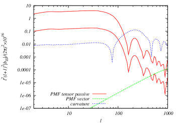
Figure 1: (color online). Absolute values of the normalized reduced CMB bispectra given by Eq. (21) for $\ell_{1}=\ell_{2}=\ell_{3}$. The lines correspond to the spectra of tensor passive modes (red solid lines), vector modes Shiraishi et al. (2010a) (green dashed line), and primordial non-Gaussianity with $f^{\rm local}_{\rm NL}=5$ Komatsu and Spergel (2001) (blue dotted line). The PMF parameters are fixed to $B_{1{\rm Mpc}}=4.7{\rm nG},n_{B}=-2.9$, and $\tau_{\nu}/\tau_{B}=10^{17}$ (upper line) and $10^{6}$ (lower line), and the other cosmological parameters are equal to the mean values limited from the Wilkinson Microwave Anisotropy Probe 7-yr data Komatsu et al. (2010).

In Fig. 2, we also show $b_{\ell_{1}\ell_{2}\ell_{3}}$ with respect to $\ell_{3}$ for $\ell_{1}=\ell_{2}$. From this figure, for $n_{B}=-2.9$, the normalized reduced bispectrum is evaluated as

$$\ell_{1}(\ell_{1}+1)\ell_{3}(\ell_{3}+1)|b_{\ell_{1}\ell_{2}\ell_{3}}|$$

$$\qquad\sim(130-6)\times 10^{-16}\left(\frac{B_{1\rm Mpc}}{4.7\rm nG}\right)^{6}~{},$$ (25)

where the factor $130$ corresponds to the $\tau_{\nu}/\tau_{B}=10^{17}$ case and $6$ corresponds to $10^{6}$. It is also clear that $b_{\ell_{1}\ell_{2}\ell_{3}}$ for $n_{B}\sim-3$ dominates in $\ell_{1}=\ell_{2}\gg\ell_{3}$. Comparing this with the approximate expression of the bispectrum of local-type primordial non-Gaussianity in curvature perturbations as Riotto (2008)

$$\ell_{1}(\ell_{1}+1)\ell_{3}(\ell_{3}+1)b_{\ell_{1}\ell_{2}\ell_{3}}\sim 4\times 10^{-18}f^{\rm local}_{\rm NL}~{},$$ (26)

the relation between the magnitudes of the PMF and the nonlinearity parameter of the local-type configuration $f^{\rm local}_{\rm NL}$ is derived as

$$\left(\frac{B_{1\rm Mpc}}{1\rm nG}\right)\sim(1.22-2.04)|f^{{\rm local}}_{\rm NL}|^{1/6}~{}.$$ (27)

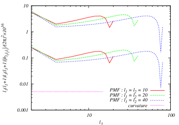
Figure 2: (color online). Absolute values of the normalized reduced CMB bispectra given by Eq. (21) and generated from primordial non-Gaussianity in curvature perturbations given by Eq. (26) as a function of $\ell_{3}$ with $\ell_{1}=\ell_{2}$. Each parameter is identical to the values defined in Fig. 1.

Using the above equation, we can obtain the upper bound on the PMF strength. As shown in Fig. 1, because the tensor bispectrum is highly damped for $\ell\gtrsim 100$, we should use an upper bound on $f^{\rm local}_{\rm NL}$ obtained by the current observational data for $\ell<100$, namely $f^{\rm local}_{\rm NL}<100$ Smith et al. (2009). This value is consistent with a simple prediction from the cosmic variance Komatsu and Spergel (2001). From this value, we derive $B_{1\rm Mpc}<2.6-4.4{\rm nG}$ These are $4-2$ times stronger than vector-modes bounds Shiraishi et al. (2010a).

In this paper, we study the CMB temperature bispectrum generated from the tensor anisotropic stresses of PMFs and find a new constraint on the magnetic field magnitude when the PMF spectrum is close to a scale-invariant shape. Although there is a touch of uncertainty in the production epoch of PMFs, this bound is tighter than ones obtained by the CMB power spectra Paoletti and Finelli (2010); Shaw and Lewis (2010a). Although this limit is weaker than a rough bound from only the scalar passive modes Trivedi et al. (2010) due to the rapid decay of the tensor bispectrum at small scales, the significant amplitude at large scales will have a drastic impact on the precise calculation of the limit on PMFs, including the scalar, vector, and tensor-mode contributions.

In our previous studies and the above analysis, we find that tensor (vector) modes dominate at large (small) scale, not only in the power spectrum but also in the bispectrum. It is also expected that the scalar mode dominates at the intermediate scale. Therefore, using this scale-dependent property, we will also constrain a spectral index of the PMF spectrum in addition to the magnetic strength. These reasonable bounds will be obtained by considering the CMB temperature and polarization bispectrum of autocorrelations and cross-correlations between scalar, vector, and tensor modes in the estimation of the signal-to-noise ratio.