A periodic representation of the interface for the volume of fluid method
Abstract
We extend the volume of fluid method for the computation of two-phase flow to a higher order accurate method in two dimensions. The interface reconstruction by the PLIC method is thereby replaced by a periodic interface reconstruction. The advection step is reformulated and extended to higher order in order to account for the present interface representation. This periodic interface reconstruction describes the interface in terms of higher order periodic B-splines. Numerical tests verify that the theoretical order of convergence is indeed exhibited by the present method.
keywords:
B-Splines , Two-phase Flow , VOF , High Order Accuracy1 Introduction
Two-phase flow can be found in many industrial applications.
A popular method for the computation of two-phase flow is
the volume of fluid method (VOF) [20, 2].
The volume fraction, the central object of the volume of fluid method,
denotes the ratio of the volume (area in 2D) occupied by one phase in
a cell of the computational domain to the cell volume (cell area in 2D).
The volume of fluid method can be subdivided into two steps: the
interface reconstruction step and the advection step. The interface
reconstruction step computes the interface position at time using the
volume fraction field at time . The advection step advects the volume
fraction field from time to time using the
reconstructed interface at time . The volume of fluid method
has its origins in the works of [7] and [14].
Substantial improvement of the interface reconstruction has been achieved
with the piecewise linear interface computation (PLIC) method by
Youngs
[26] in 1982. However, the resulting interface is
approximated by piecewise straight lines which makes it necessary to
estimate the curvature by additional approximation schemes,
for example the height function method
[6, 10, 9, 11].
In order to obtain a more smooth interface, Price et al. in 1998 [17] derived a method
replacing the straight lines by parabolas.
Due to the fact
that a numerical minimization has to be performed in each cell to find all the
coefficients of the interface parabola, the method enjoys less popularity. More
recently, in 2004, Lopez et al. [12]
used a parametric cubic spline interpolation
through the midpoints of the PLIC interface lines and obtained a smoother
description of the interface. However, although cubic splines are known to
interpolate a function with fourth order accuracy, their method inherits the
second order accuracy of the PLIC method for the test cases presented in
[12] since it is based on the same
approach. A further development of this interface reconstruction
using splines to improve the interface obtained by the piecewise lines
of the PLIC method has been presented in [8]
using quadratic splines. Both approaches are, however, based on the PLIC method
for reconstruction and advection and share therefore also the drawbacks of
the PLIC method. Another approach replacing this time the PLIC method has been
presented in [23, 22, 24],
where the interface is divided into segments and each segment is reconstructed
globally. This allowed for a more accurate description of the interface.
A drawback of this method is however the need to choose a division of the
interface into segments.
In the present discussion we shall modify the approach presented in
[23, 22, 24] by deriving a
periodic description of the interface separating two immiscible
liquids in two dimensions. The present method is, as the method in
[23, 22, 24],
a global method opposed to the PLIC method which uses only local information.
The interface in the present discussion
is represented indirectly by two functions depending on a periodic parameter.
The actual position or other quantities, such as the normal or
the local curvature at the interface, are then derived from these
two functions. The advection step is adapted to the present
interface representation.
The present discussion is organized as follows:
The present interface representation is derived in the next section,
section 2. Periodic B-splines are used to approximate
the interface, cf. section 3.
In section 4,
the advection step is presented. The numerical verification is done
in section 5. Finally, the present
discussion is concluded in section 6.
2 A periodic representation of the interface
In the present discussion we treat the case of a two dimensional drop of blue fluid enclosed in red fluid, cf. figure 1. The red fluid occupies the domain , whereas the blue fluid occupies the domain . These two domains are separated by a common boundary, the interface . The central problem of the volume of fluid method is to compute the temporal evolution of the interface when subjecting the fluids to a velocity field :
| (1) |
Since we are dealing with incompressible fluids, the velocity is solenoidal. In the present discussion we assume that the interface can be described by a periodic line . We exclude topological changes in the present discussion. In addition any third phase should not be present in order to avoid contact points. We also assume the line to be sufficiently regular. As for polygons, cf. [1], the area of a domain , enclosed by a line , can be computed by means of a function :
| (2) |
where is the position vector of a point. The divergence of (2) is unity, as can be verified straightforwardly. Having now a periodic parametrization of the line :
| (3) |
the area of can be expressed by:
| (4) |
where the periodicity of the line has, without loss of generality, been chosen to be . It is, in addition, implied that the tangential on points in counter clockwise direction. We now define two functions , resp. by:
| (5) | |||||
| (6) |
The derivatives of , resp. are then given by:
| (7) | |||||
| (8) |
Since the position of a point on the interface is periodic in , we conclude that the derivatives , resp. are also periodic in . The position of a point on the interface on the other hand can then be recovered by the following expressions:
| (9) | |||||
| (10) |
Integrating equations (9) and (10) with respect to gives us then the final result:
| (11) | |||||
| (12) |
where is the position of the interface for . In order for equations (9) and (10) to be well defined we have to choose a coordinate system having the region in the positive quadrant sufficiently far from the origin. The area included by the interface is then given by:
| (13) |
The strategy of the present method is to represent the interface of the drop by the functions , resp. and to obtain the position of the interface by formulae 11, resp. 12. A normal on the interface is then given by:
| (14) |
and the curvature can be found via
| (15) |

3 Interpolation by periodic B-Splines
As mentioned above, instead of representing the interface position directly by B-splines, as for instance done in [25] in the framework of front-tracking methods or in [12] for the volume of fluid method, we represent the interface by the two functions , resp. , equations (5) resp. (6), defined on the interval . We use a uniform discretization of the interval , meaning that we choose knots :
| (16) |
dividing the interval into sections of equal length. Periodic B-splines can actually handle more flexible discretizations, which could be used to distribute points to regions of interest. However, in the present discussion we restrict us to the uniform case. Having now the knots , , the periodic basis spline of order is obtained recursively by, see for instance [13, 15]:
| (17) | |||||
| (20) |
The basis spline has finite support . Therefore representing the function to interpolate as a linear combination of the periodic basis splines :
| (21) |
leads to a cyclic banddiagonal system with bandwidth for the unknown coefficients . In the present discussion we will only use odd order B-splines. The function values for interpolation are then taken at the knots [15]:
| (22) |
For the resulting interpolation we have the following bound, see for instance [13]. If and if and the interpolating spline of order are periodic on , the following bound holds:
| (23) |
where and the constant is given by:
| (24) |
This implies that if choosing B-splines of order the interpolation
will have an order of accuracy with respect to the grid spacing.
The cyclic banddiagonal system resulting from (21)
can be solved efficiently by means of a
banddiagonal solver in combination with the Woodbury formula
[16].
The function , equation (6), is periodic and can thus directly be interpolated by periodic B-splines. However, the function is not periodic but takes different values at the right and left boundary of the interval :
| (25) |
where is the area of the drop. The derivative is, however, periodic. In order to use periodic B-splines to interpolate the function , we define a periodic function by:
| (26) |
which is then interpolated using periodic B-splines. Once we have an approximation to the functions , resp. , equations (5) resp. (6), we evaluate the integrals
| (27) | |||||
| (28) |
from equations (9), resp. (10) by Gaussian quadrature [18], in order to compute the position by means of equations (11), resp. (12). This will, however, introduce additional numerical error. A consequence of this is that the integrals in equations (27), resp. (28), might numerically not evaluate to zero for and . Therefore we determine first the total quadrature error , resp. by
| (29) | |||||
| (30) |
where the symbol means taking the numerical quadrature of the integral , equation (27), from to . Since B-splines are discontinuous in the derivative across the knots , we perform a Gaussian quadrature on each subinterval . In order to assure that the position, given by equations (11), resp. (12) is itself a periodic function of we replace the argument , resp. of the integrals in equations (27), resp. (28) by and defined the following way:
| (32) | |||||
| (33) |
4 Advection step
Once we are given an interface at time represented
by the two functions and , equations (5),
resp. (6), we need to formulate an advection scheme which
allows to compute the interface at time .
Before going over to the actual derivation
we introduce the notions of flux and fluxing regions.
In the present discussion we assume that the flux
through a section with end points ,
resp. can be computed for arbitrary points
and . The
flux is given by
| (35) |
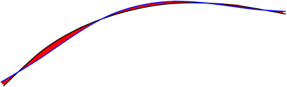
where is the volume flow and the stream function. In the present discussion the flux will be computed analytically, since we are given the analytical stream function for the benchmark tests in section 5. The flux has a geometrical interpretation, cf. figure 2. It can be seen as the signed area of the region of points passing through a line with end points , resp. from to , the fluxing region. This region is bounded by the line from to , its image at , when tracing the line back from to and the trajectories , resp. of the points , resp. . In order to trace a point from to we have to solve the following differential equation:
| (36) |
with initial condition , where is the velocity field, which is for the present benchmark tests, cf. section 5, given analytically. We solve equation (36) by the classical four stage Runge-Kutta method. For the present advection scheme it is necessary to approximate the trajectory from time to of a point . This is done by means of Lagrange polynomials on the Gauss Labatto Legendre (GLL) nodes, cf. for instance [18], on the interval . If is the number of nodes chosen, the interval is divided by the GLL nodes into sections , . Solving equation (36) successively for each point in time , will give us a set of interpolation points:
| (37) |
where . The trajectory can then be approximated by:
| (38) |
where is the Lagrange polynomial.
The advection step is sketched schematically in figure 3.
Having the interface at time represented by the
functions , resp. , equations (5), resp.
(6), we choose a sequence of points on the interface ,
as depicted in figure 3. Several criteria might be
possible according to which the points might be chosen
[4].
However, in the present discussion we take the points at the
parameter values , the nodes chosen for the discretization, equation
(16). The points are computed by equations (11),
resp. (12):
| (39) |
It is known that during simulation the points on the interface
can cluster in regions of the interface if always the same points on the
interface are traced forward [3]. However, in
the present discussion we will not treat this problem but instead focus
on the general method itself.
Now that we have chosen a sequence of points on the interface
at time ,
we trace forward in time from to by
solving (36), as depicted in figure 3, giving us
the point . In the following the point
at time will be written with a tilde to
indicate that this quantity is at time . Its image
at time will
be written without tilde .
Focusing now on two consecutive points
and at time ,
we know that the area bounded by the interface at time ,
by the trajectories and of the points , resp.
, and the interface at time
must equal , as depicted in figure 3.
The flux can thus be written as a sum of integrals
along the bounding lines of the fluxing region:
| (40) |
where is the integral along the interface from to ,
| (41) | |||||
| (42) |
since we are representing the interface by means of and , cf. equation (5), resp. (6). The integral on a trajectory is given by
| (43) |
Since is a polynomial of order in , Gaussian quadrature can be used to compute the integral (43) exactly. Finally the integral on the interface at time can be written as
| (44) | |||||
| (45) |
where is the unknown function representing the interface at time . We can solve equation (40) for :
| (46) | |||||
| (47) | |||||
| (48) |
since we have chosen .
A kind of similar idea is used for surface marker particles
in order to correct for area loss during advection, cf.
[25]. In the present method it is, however, not used
as a correction but as the principle behind the advection step.
The interpolation points
| (49) |
are then interpolated as mentioned in section 3 to give an interpolant of resp. for the interface at time . The area of the drop is conserved, since for all time steps. However, this conservation property should be understood in a less strict sense, since the quadrature errors , resp. in equations (29), resp. (30) will lead to the fact that the area bounded by the actual interface given by the points computed by equations (11) and (12) can be different from . In addition, errors can lead to the development of self intersections of the interface, cf. figure (4). Area conservation should rather be understood as the underlying principle of the method which is implemented through the function which, together with , can be seen as a kind of generating function for the position.


5 Numerical verification
The numerical verification of the present third order volume of fluid method is done by three classical benchmark tests, the reversed single vortex test by Rider and Kothe [19], Zalesak’s slotted disk test [27] and the deformation field test [21]. However, before going over to the numerical verification, we have a glance at the definition of the numerical error.
5.1 Numerical Error
The error norm in the present discussion measures the area difference between the numerical interface and the exact interface as depicted in figure 5. The error is computed using the position of the interface computed by means of equations (11), resp. (12) and not by means of the function , equation (5). The integration between the numerical solution and the exact interface in order to compute the area difference is done by means of Gaussian quadrature, where we ensured that the quadrature error is negligible compared to the numerical error of the method. The order of convergence between two resolutions and , is computed using :
| (50) |
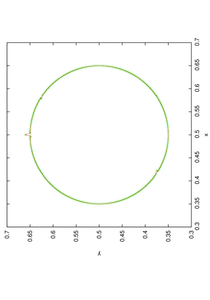
5.2 Numerical verification part 1
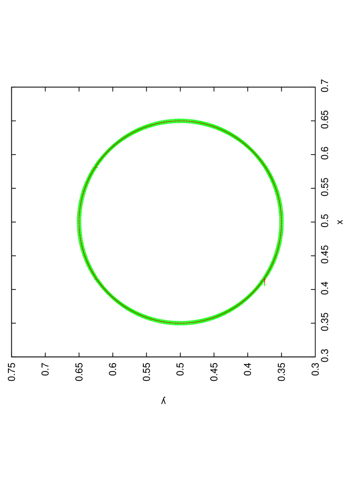
The setup of the reversed single-vortex test of Rider and Kothe [19] consists of a circular drop of radius placed at position in a unit square box. The velocity field is obtained by means of the following stream function :
| (51) |
where is the period at which the drop has returned to its initial position. Thereby its interface at time should match the initial circle. The discrepancy between the numerical interface at time and the exact circle serves as a measure of the numerical error. As initial condition we used
| (52) | |||||
| (53) |
where . As mentioned in section 3, we
divided into equidistant sections. We performed three
series of tests for , and .
The results of these tests are shown in figures
6, 7, 8,9,
10,11,12,
13,14,
15,16
and tables 1, 2,
3. For all simulations we chose for the
approximation of the trajectories for the advection step, cf. section
4. Depending on the order of the B-spline interpolation
we chose a different value for the time steps in order
to make the error contribution due to the advection step subdominant compared to
the error contribution of the interface Reconstruction. The advection step
itself can handle quite large time steps without displaying any sign of
instability. All simulations
were performed using B-splines of order . For the
time step was chosen , for , ,
and for , . The time step was kept fixed
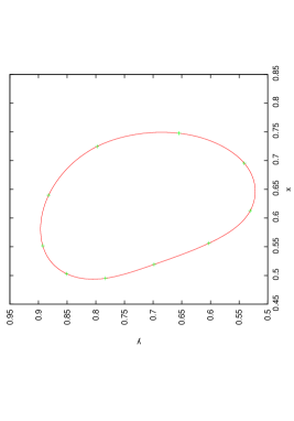
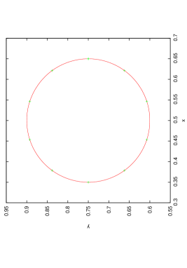
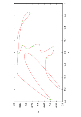
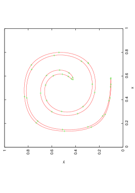
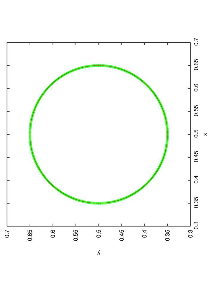
at these values even when going over to finer resolutions. In figure
6 the resulting position of the interface is shown for
and in the case , and
a resolution of . The interface is well resolved and does not
display any visual disturbances such as bumps or oscillations at maximum
deformation and when it has returned to its initial position at .
The same observation can be made for the
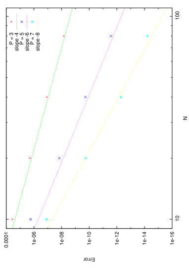
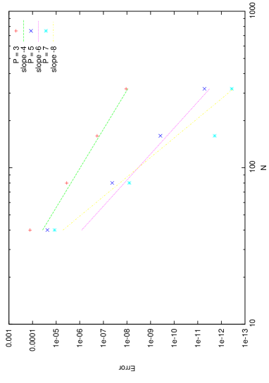
case , cf. figure 8. Concerning the convergence of the
method for these two cases, e.g. and , cf. figures
7, resp. 9 and
tables 1, resp. 2, we observe that the
order of convergence corresponds approximately to the theoretical value of
, cf. equation (23). For and fine
resolutions the error does not further decrease because of the round off limit.
In addition, for the case when going from to , we
observe a sudden jump in the convergence, cf. figure 9 and
table 2, for and . This phenomenon of
accelerated convergence is even more pronounced in the case , cf.
figure 12 and table 3. An explanation
for this sudden increase in convergence
might lie in a underresolution of the problem for coarse
resolutions , meaning that when increasing , keeping fixed at
a small value no important gain in accuracy is observed. However, if the
resolution is finer, i.e. large values of , increasing will
almost lead to spectral convergence, i.e. faster than algebraic. This points
to the eventuality of having insufficient sampling of the signal,
i.e. an aliasing error.
This is different to classical spectral methods such as methods based on
Chebyshev or Legendre polynomials for which increasing the approximation
order introduces an increase of spatial resolution by
increasing the number of Gauss points. Periodic
B-splines on the contrary offer the possibility of increasing and
independently with the consequence of having eventually a
persisting aliasing error when only increasing .
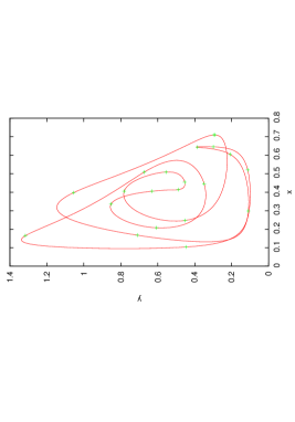
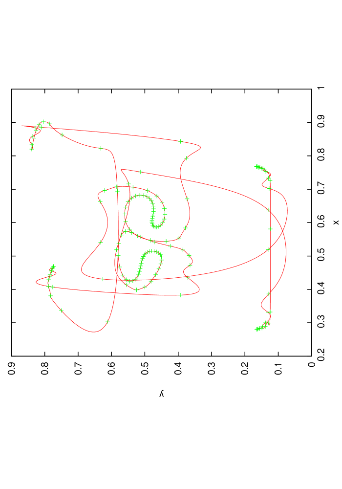
Even worse a
underresolved simulation can lead to an entirely wrong solution
by the present method,
as can be seen in figure 10. Here and
the resolution was fixed at 20 (). For still a
few structures of the correct solution are recognizable, however for
the picture has entirely deteriorated. If underresolved, the numerical solution
can display self intersections. This indicates that the present method is less
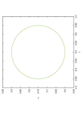
robust to underresolution. However, for well resolved cases, which for
the case start at only 40 knots, cf. figure
11, the present numerical scheme produces a very accurate
result.
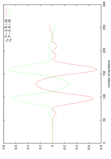
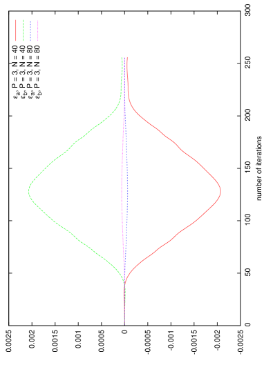
Concerning area conservation, we observe
from figure 13 that the value
is, apart from round off contributions, equal to the initial area of the
drop. However, the quadrature errors , resp. ,
equations (29), resp. (30), can become rather
important during simulation, as for instance for the
underresolved case , and , cf. figure
14, indicating a possible
discrepancy between the actual area of the drop and .
For well resolved cases the quadrature errors are smaller, cf.
figure 15, but seem to increase with
increasing deformation of the drop.
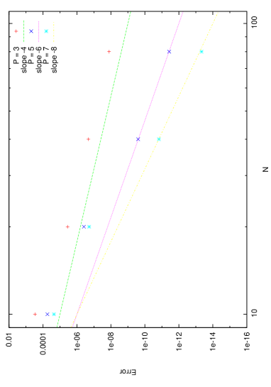
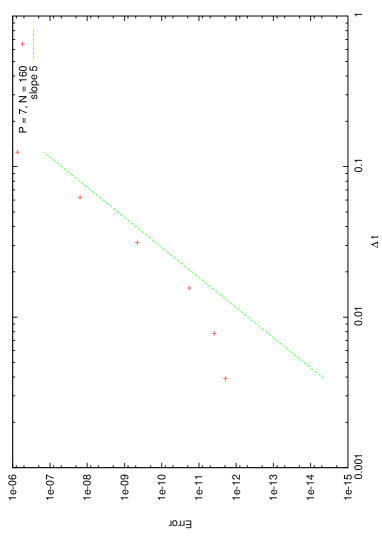
As a last numerical experiment we investigated the accuracy of the
advection scheme derived in section 4.
By fixing the number of Gauss Labatto Legendre nodes to ,
the interpolating polynomial has order 4 for which reason we
expect the advection scheme to converge with order
accuracy with respect to the time step .
In order to observe the error contribution by the advection
scheme, we chose a B-spline of order and a spatial
resolution of , such that the error contribution by
the interface representation is subdominant. Decreasing
the time step leads indeed to a fifth order
convergence of the numerical error up to the point at which
the error contribution by the interface representation
becomes dominant, cf. figure 16.


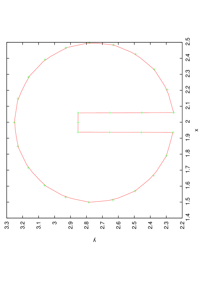
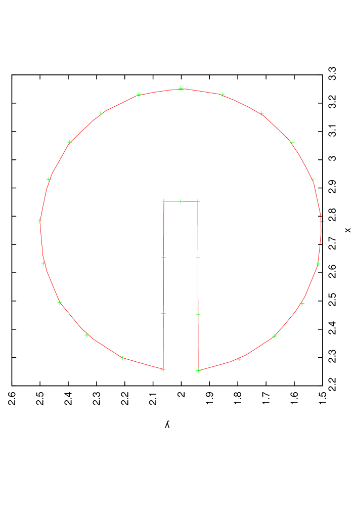
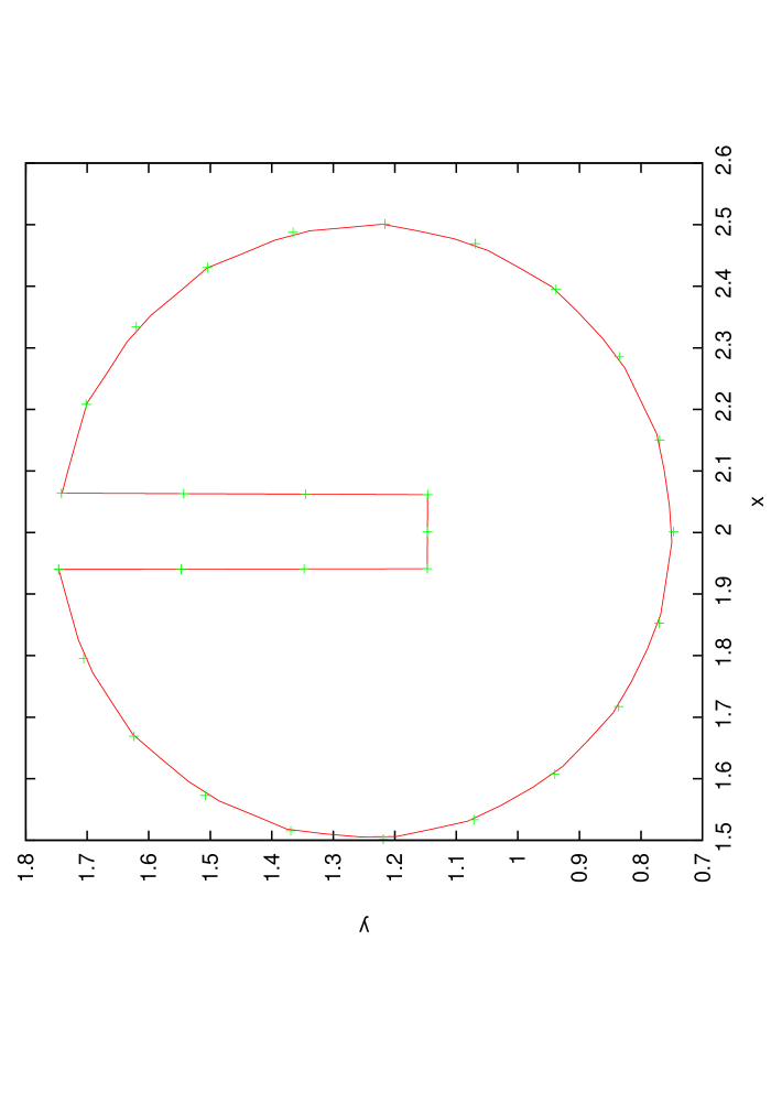
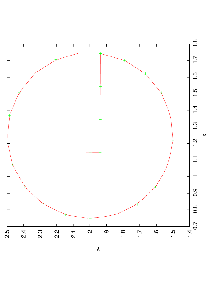
5.3 Numerical verification part 2
The slotted disk rotation test of Zalesak [27] uses a solid body rotation to advect a slotted disk. The stream function is given by
| (54) |
where is chosen in such a way as to allow a complete rotation of the drop in iterations. The computational box is four by four and the drop has a radius of . It is situated at . The coordinates of the four corners of the slot are given by:
| (55) | |||||
| (56) | |||||
| (57) | |||||
| (58) |
As an initial condition we chose a description of the initial interface by means of four functions , defined the following way:
| (59) | |||||
| (60) | |||||
| (61) | |||||
| (62) |
where and . The function is composed by means of these four functions.
| (64) |
The parameter takes values in the interval this time. We discretized this interval in such a way that the corner positions of the slot are at knots of the discretization. The function is then interpolated at these knots. The function is handled likewise, with given by:
| (65) |
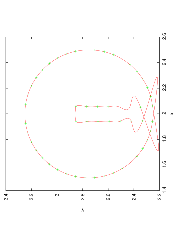
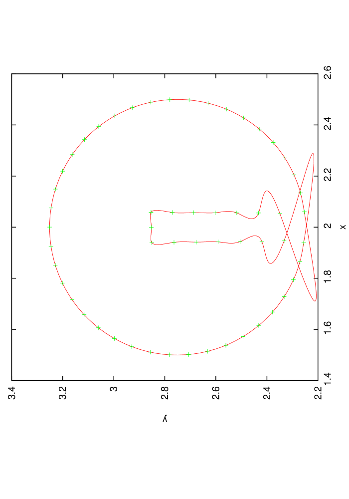
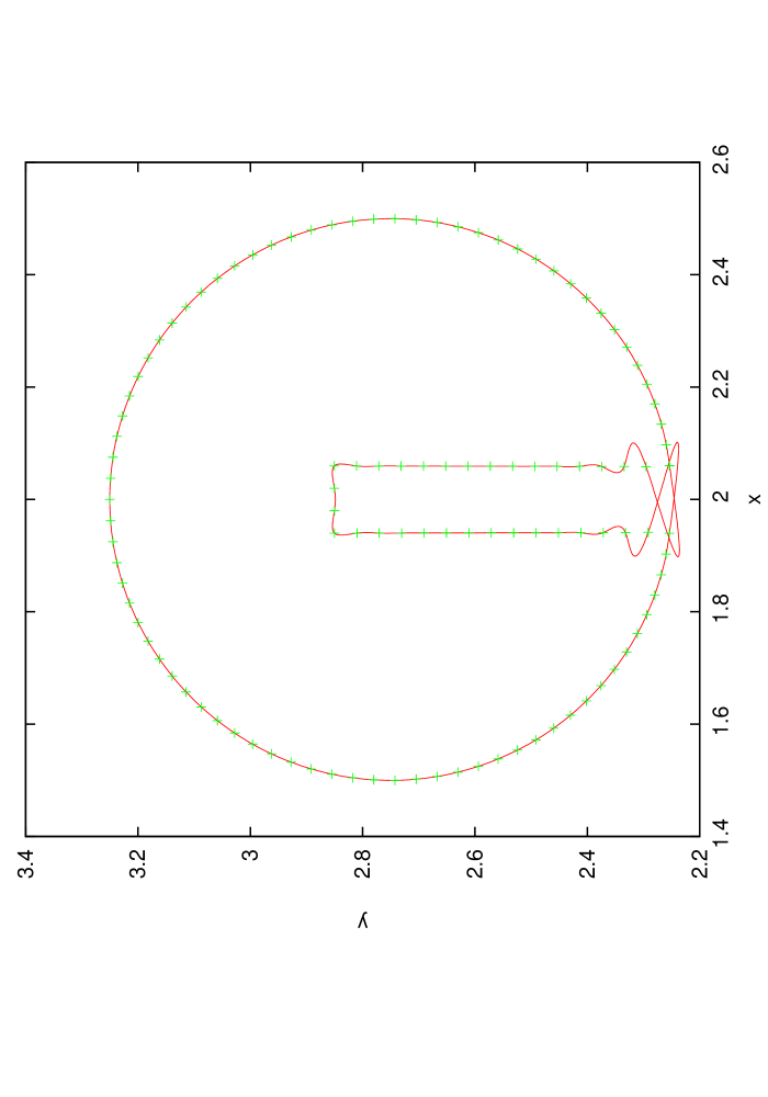
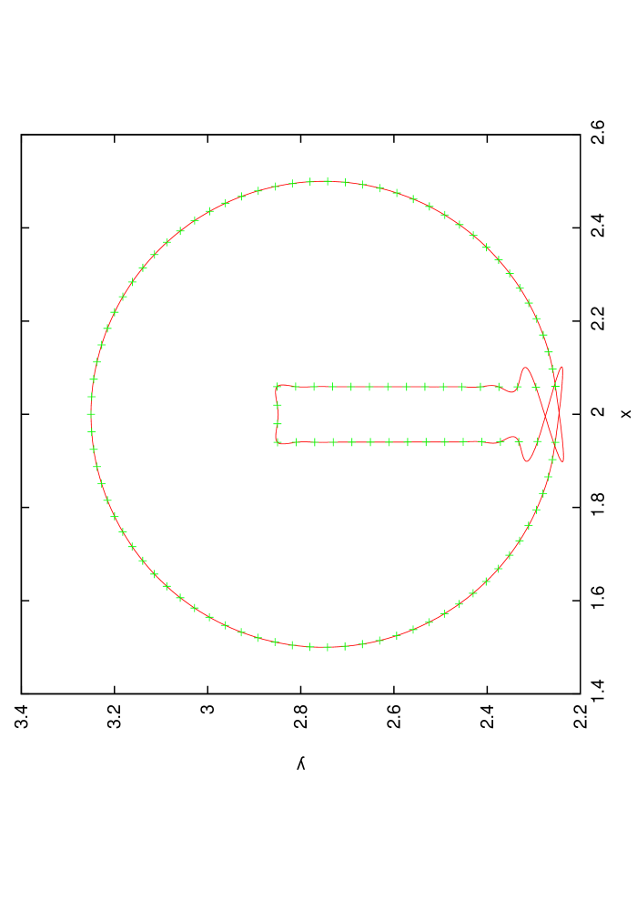
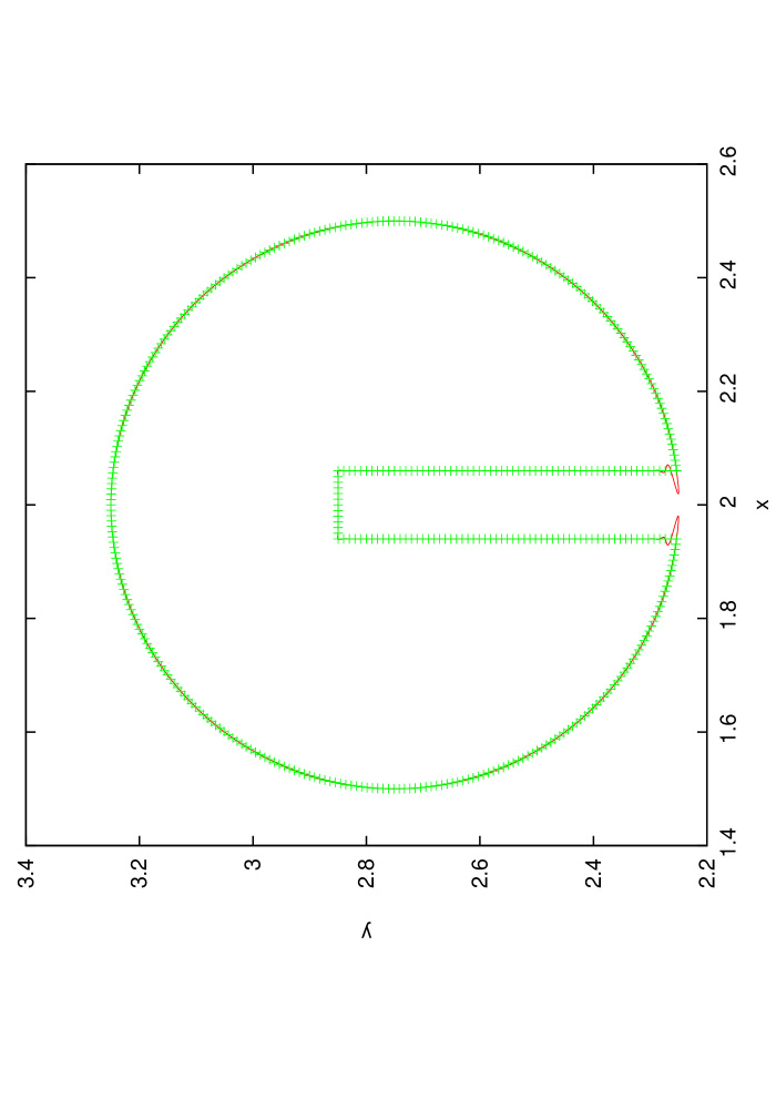
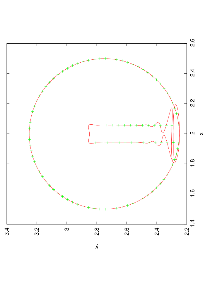
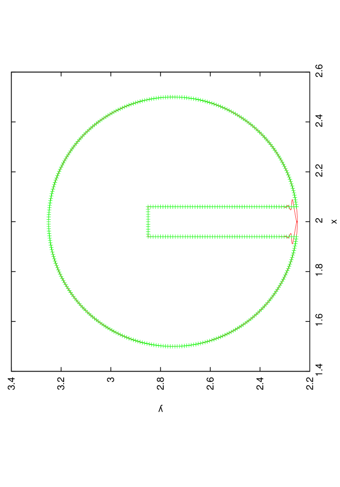
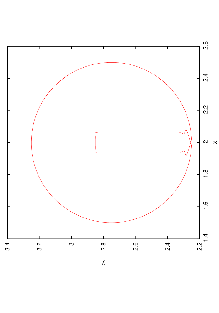
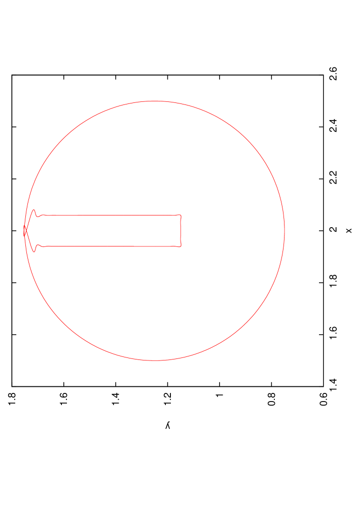
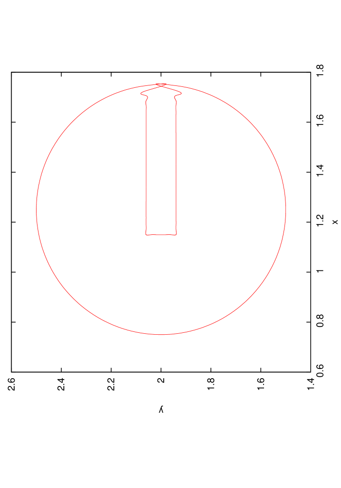
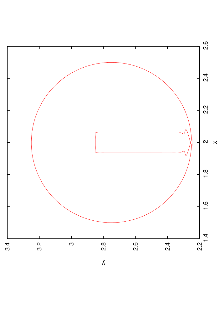
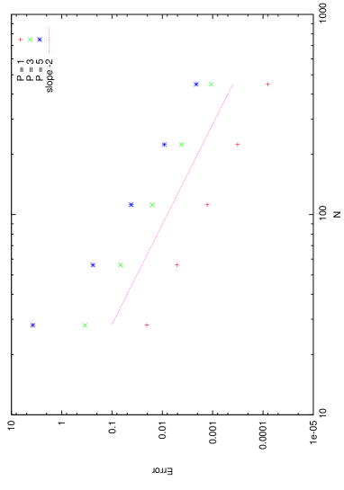
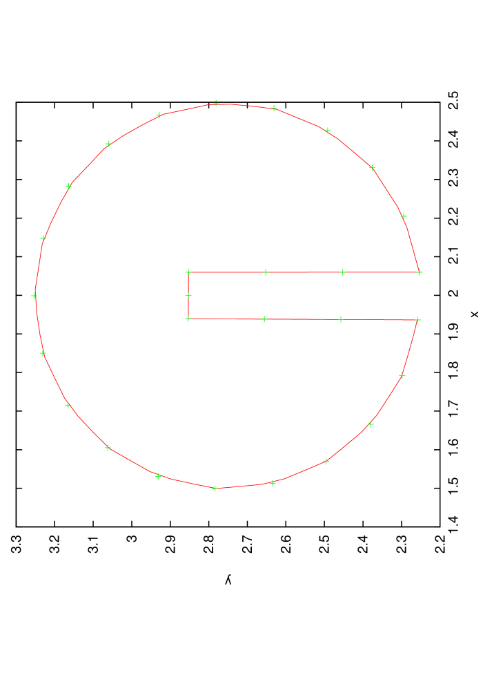
The initial condition is only because of the kinks at the corners of the slot. Although using high order periodic B-splines, we expect the convergence rate therefore to be of only second order at most. In addition, discontinuities can give rise to the development of spurious oscillations of the interpolant at these discontinuities, the so called Gibbs phenomenon [5]. The higher the order of the periodic B-splines the further these spurious oscillations spread along the interface, as can be seen when comparing figures 17 and 18, where we compare the interface position at time and , after one rotation, for different resolutions. Intermediate steps are shown for and in figure 19, indicating that the main contribution to the overall error does indeed not come from the advection but from the interpolation of a function with discontinuities in its first derivative. The order of convergence is reduced to second order no matter the order of the B-spline interpolation, cf. figure 20, resp. table 4. The absolute error is even larger for higher order B-spline interpolation, due to the larger spurious oscillations. We remark that choosing an order for the B-spline interpolation gives us a PLIC like description of the interface, which for the present benchmark test produces more accurate results since it only requires continuity of the function to be interpolated. This leads to the result that for the slot stays sharp during the entire simulation as can be seen in figure 21.
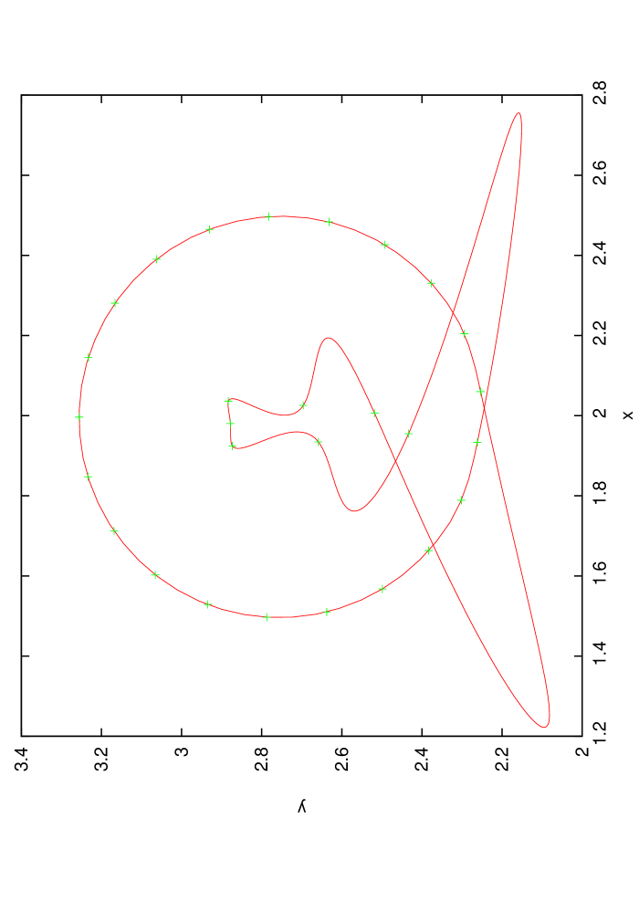
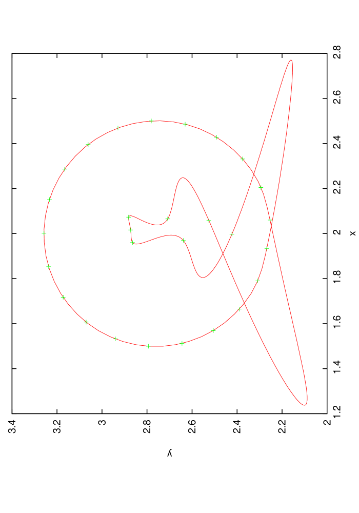


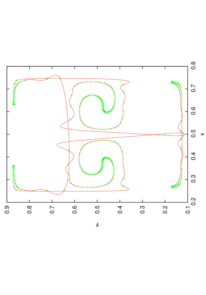
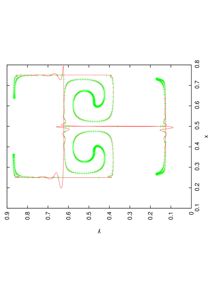
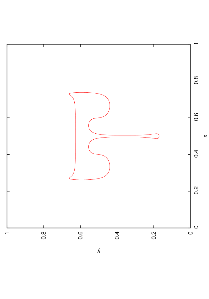
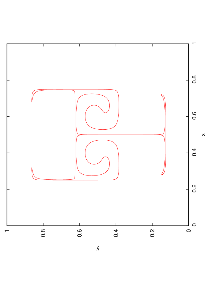
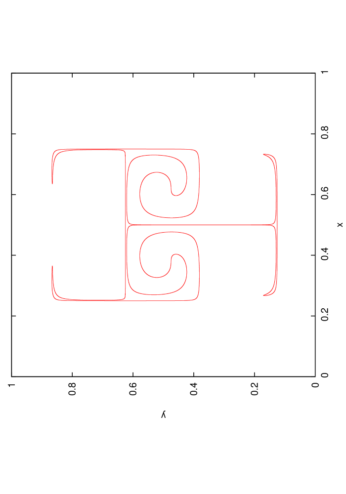
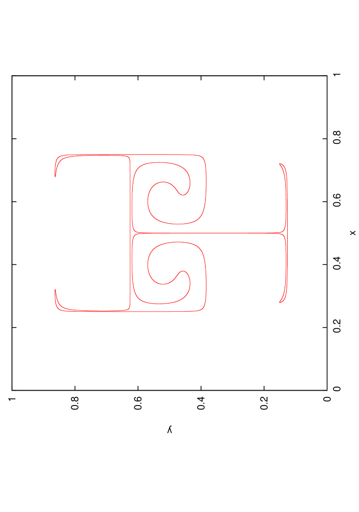
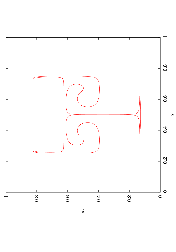
5.4 Numerical verification part 3
The deformation field test [21] uses the following stream function:
| (66) |
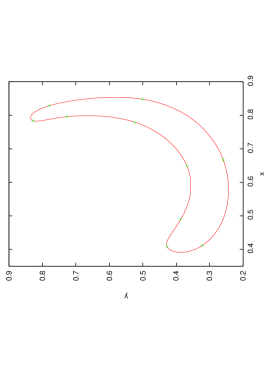
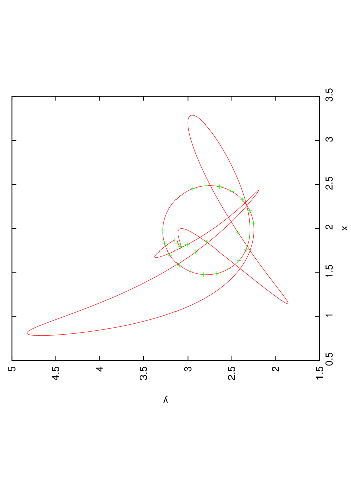
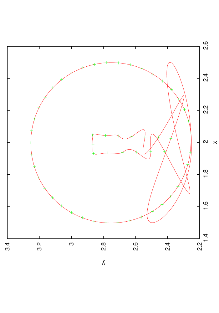
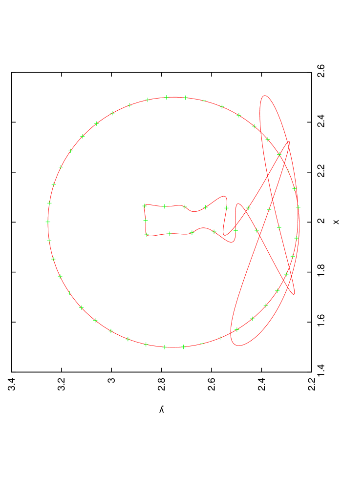
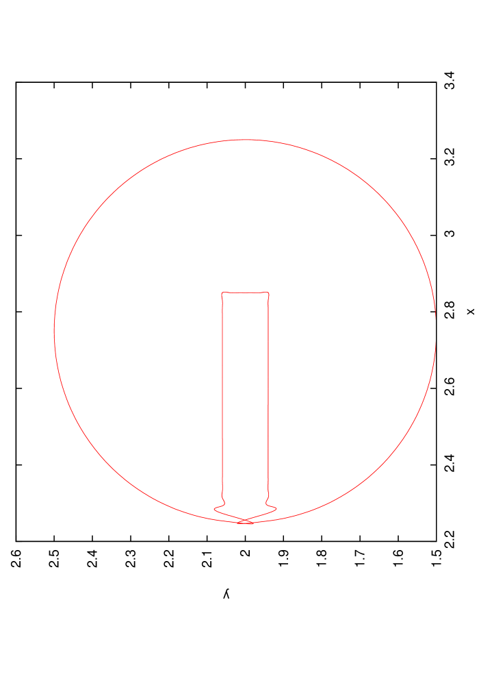
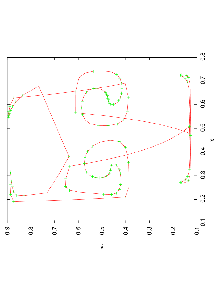
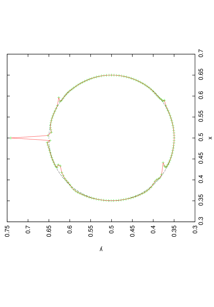
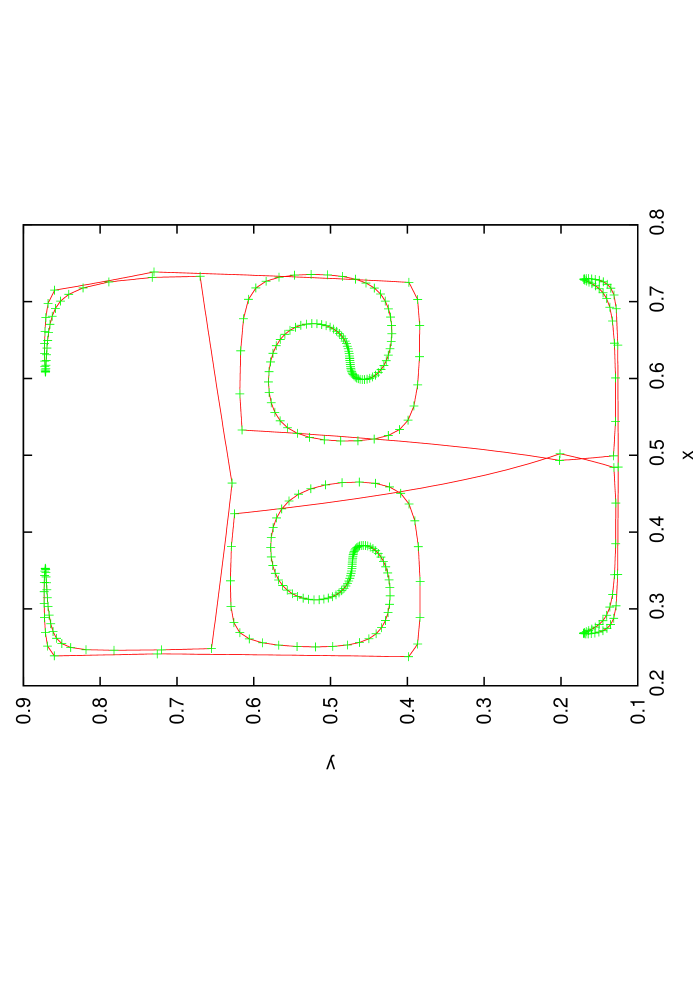
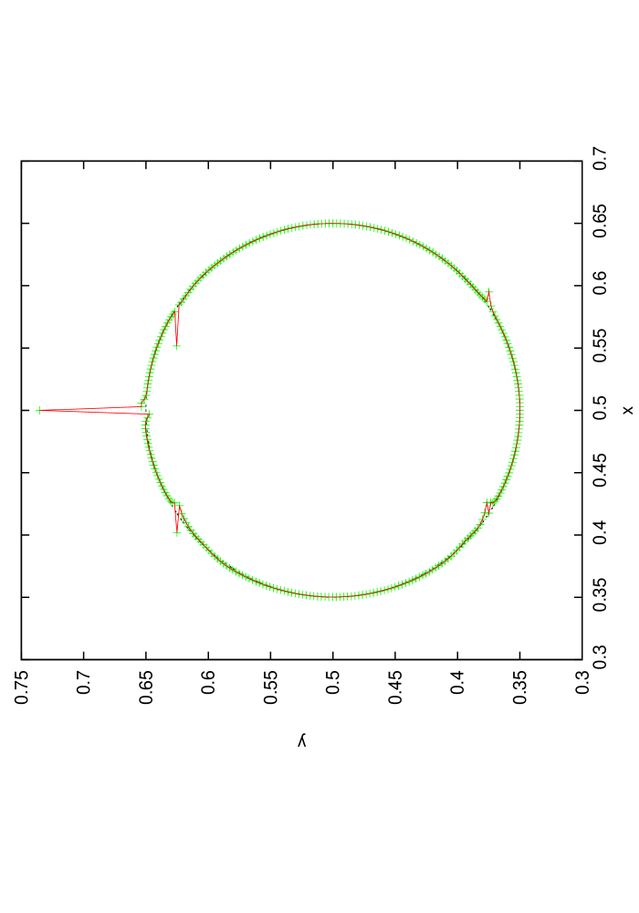
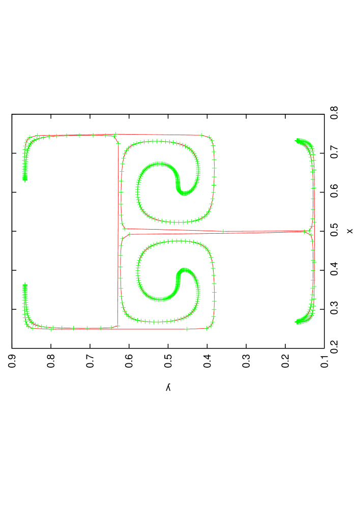
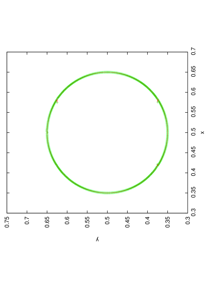
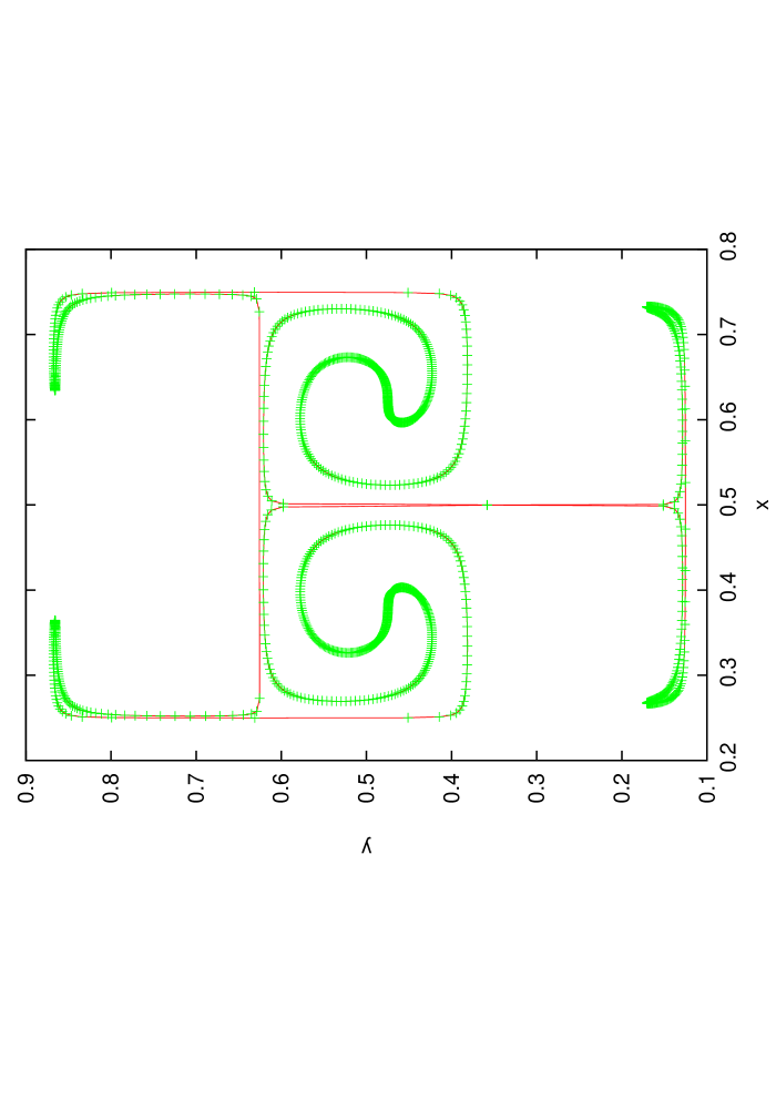
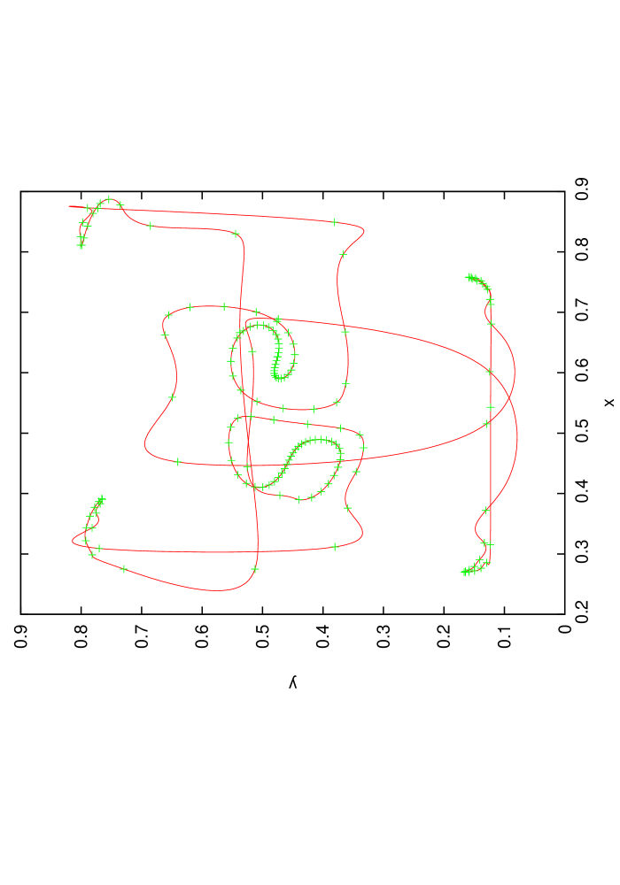
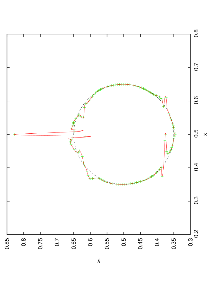
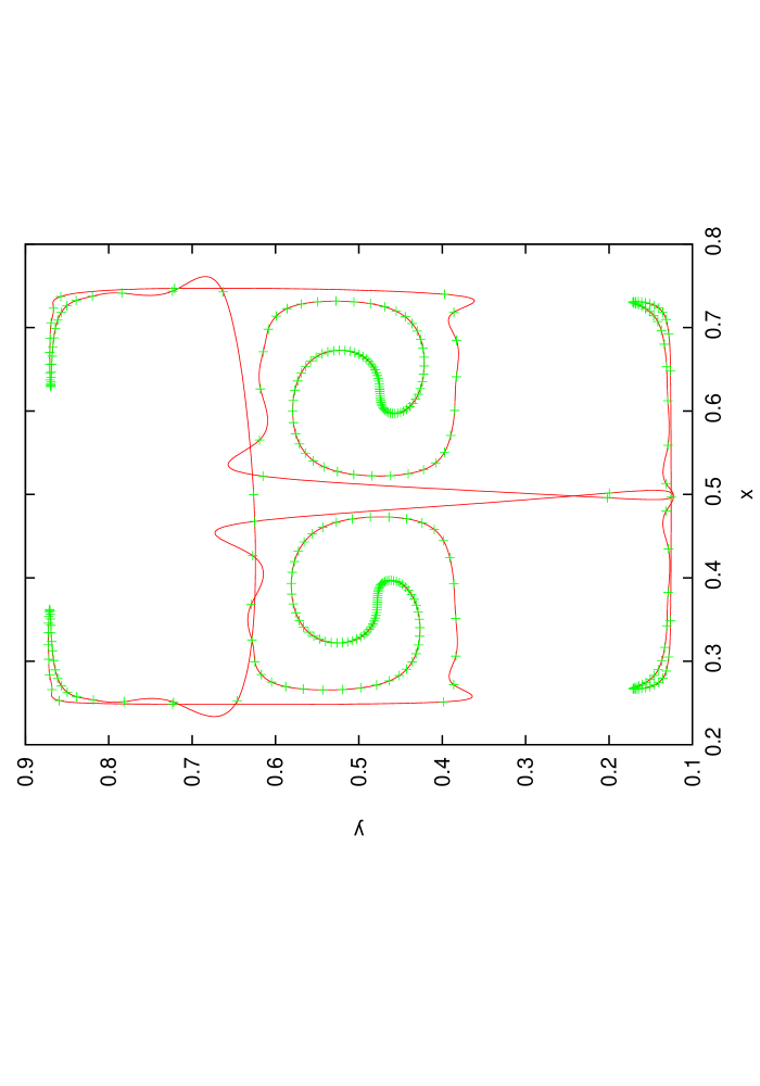
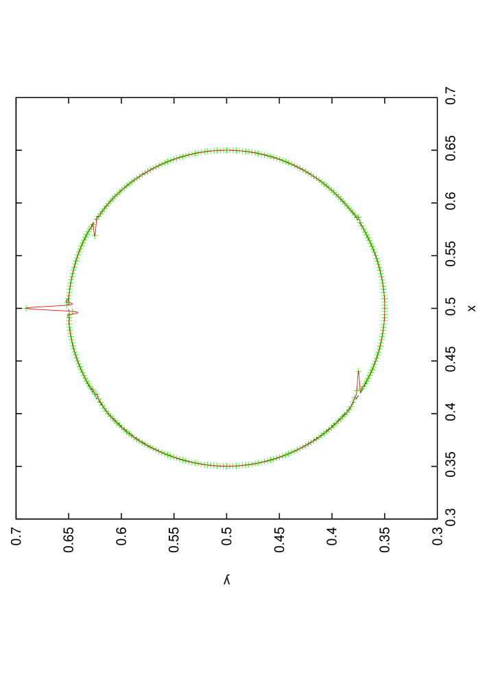
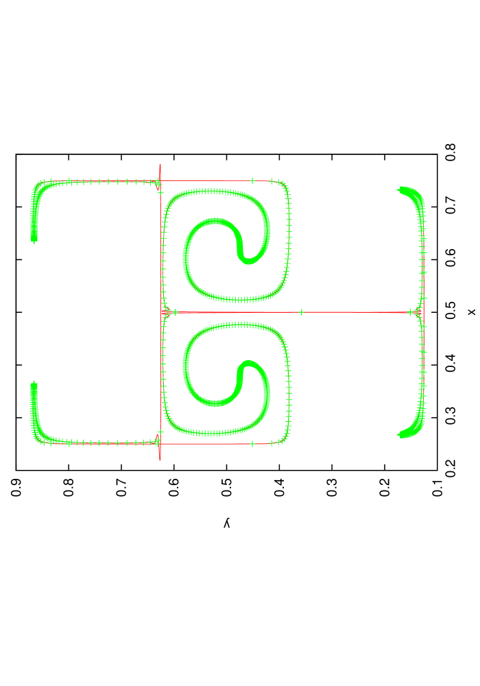
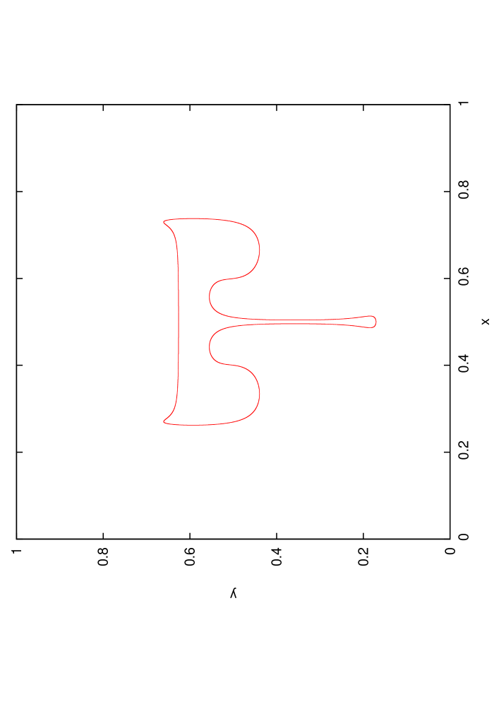
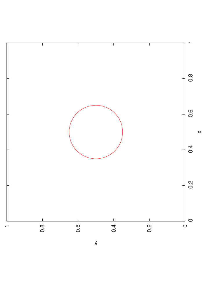
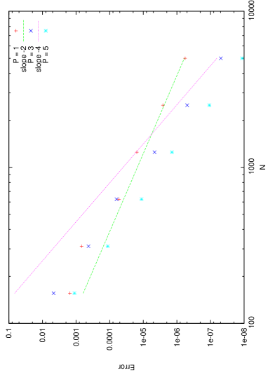
where is the number of vortexes in the computation domain and chosen to be to match the geometry used in [28, 24], as was the period with . The computational domain is a square box of side length one. A drop of radius has its center at at time . Since the flow is reversed after the drop returns to its initial position at assuming its initial shape. As initial condition we used the same functions , resp. , as for the Rider-Kothe single vortex test, equations (52-53). We performed a series of tests with , and . The time steps were chosen for and and for . This was, as before, done in order to make the error contribution by the advection step subdominant. This benchmark test is relatively difficult since the interface develops regions with very small local radii of curvature. In addition, at some parts the drop becomes very thin. The results of the present method applied on this benchmark test can be seen in figures 22 for , 23 for , and 24 for . In these figures we depicted the graph of the interface at maximum deformation and after the drop has returned to its initial position at for different resolutions. For low resolutions the graph at maximum deformation () does only capture the coarse features of the solution for all three orders , and . In addition, at regions were the resolution is low but the curvature high, the numerical solution seems to develop a kind of Gibbs phenomenon for and , as for Zalesak’s slotted disk rotation test. These oscillations become smaller as the resolution increases. When the drop has returned to its initial position we observe that the interface develops spikes at those regions where the resolution was low at maximum deformation. This is due to the fact that as the error is larger in these regions a point might fall into the wrong vortex and be traced to a different location. These spikes become smaller with increasing resolution and increasing order of the interpolating B-spline . For finer resolutions, , the final position is extremely close to the exact solution. However, at maximum deformation some wiggles can be observed for both and , indicating that measuring the error at maximum deformation might give a better estimate of the accuracy of the present method than measuring it at the final position. For and the wiggles have disappeared, as can be observed from figure 25. Concerning the order of convergence, cf. figure 26 and table 5, the present method seems to converge at a lower speed both for and for . This might have its origin in the spurious oscillations which might prevent the method from converging at the right rate. Grid adaptation or remeshing redistributing the points to regions were needed, as mentioned in section 3, might be advantageous for this benchmark test. Nevertheless, an order of convergence between three and four with respect to the spatial resolution for this benchmark test is quite acceptable.


6 Conclusions
In the present discussion we derived an alternative formulation for the interface representation for the volume of fluid method. The interface is represented in a periodic fashion by two functions and , from which the position of the interface can be calculated. These two functions are approximated by periodic B-spline interpolation which allows a systematic extension to higher order accuracy with respect to the grid spacing. The advection scheme has been simplified and extended to higher order accuracy with respect to the time step. Numerical verification indicates that the present scheme has indeed the order of convergence predicted by the theory. This allows for very accurate simulations with a limited number of knots. However, if the sampling rate is too small, the present scheme can break down, providing a numerical solution far away from the exact one. In addition, for discontinuities in the first derivatives at a point on the interface, or at regions of the interface with poor resolution and high curvature, the present method can display a kind of Gibbs phenomenon. Taking a lower order B-spline interpolation can in this case provide more appealing results. A remeshing or adaptive grid approach could increase the efficiency of the algorithm. In addition, such an approach might furnish a way to simulate topological changes such as coalescence or drop break up. The extension to three dimensions is also left for future research.
7 Acknowledgment
Thanks goes to Claudio Walker for interesting discussions. The author is grateful to Bernhard Müller for guidance and supervision.
References
- [1] J. Arvo, editor. Graphics Gems II. Morgan Kaufmann Academic Press, San Diego, 1991.
- [2] D. J. Benson. Volume of fluid interface reconstruction methods for multi-material problems. Applied Mechanical Review, 55(2):151–165, 2002.
- [3] T. Bjøntegaard and E. M. Rønquist. Accurate interface-tracking for arbitrary lagrangian-eulerian schemes. Journal of Computational Physics, 228:4379–4399, 2009.
- [4] T. Bjøntegaard, E. M. Rønquist, and Ø. Tråsdahl. High order interpolation of curves in the plane. submitted, 2009.
- [5] R. Courant and D. Hilbert. Methoden der Mathematischen Physik I. Springer-Verlag, Berlin, 1924.
- [6] S. J. Cummins, M. M. Francois, and D. B. Kothe. Estimating curvature from volume fractions. Computers and Structures, 83:425–434, 2005.
- [7] R. DeBar. Fundamentals of the kraken code. Technical Report UCIR-760, Lawrence Livermore Nat. Lab., 1974.
- [8] S. Diwarkar, S. K. Das, and T. Sundrarajan. A quadratic spline based interface (QUASI) reconstruction algorithm for tracking of two-phase flows. Journal of Computational Physics, 228:9107–9130, 2009.
- [9] P. A. Ferdowsi and M. Bussmann. Second-order accurate normals from height functions. Journal of Computational Physics, 227:9293–9302, 2008.
- [10] M. M. Francois, S. J. Cummins, E. D. Dendy, D. B. Kothe, J. M. Sicilian, and M. W. Williams. A balanced-force algorithm for continuous and sharp interfacial surface tension models within a volume tracking framework. Journal of Computational Physics, 213:141–173, 2006.
- [11] M. M. Francois and B. Swartz. Interface curvature via volume fractions, heights, and mean values on nonuniform rectangular grids. Journal of Computational Physics, 229:527–540, 2010.
- [12] J. López, J. Hernández, P. Gómez, and F. Faura. A volume of fluid method based on multidimensional advection and spline interface reconstruction. Journal of Computational Physics, 195:718–742, 2004.
- [13] G. Micula and S. Micula. Handbook of Splines. Kluwer Academic Publishers, 1999.
- [14] W. Noh and P. Woodward. Slic (simple line interface calculation). In Proceedings of the 5th International Conference on Fluid Dynamics, volume 59, pages 330–340, 1976.
- [15] G. M. Phillips. Interpolation and Approximation by Polynomials. Springer Verlag, New York, 2003.
- [16] W. H. Press, S. A. Teukolsky, W. T. Vetterling, and B. P. Flannery. Numerical Recepies in C++. Cambridge University Press, second edition, 2002.
- [17] G. Price, G. Reader, R. Rowe, and J. Bugg. A piecewise parabolic interface calculation for volume tracking. In Proceedings of 6th Annual Conference of the Computational Fluid Dynamics Society of Canada, Victoria, British Columbia, 1998. University of Victoria.
- [18] A. Quarteroni, R. Sacco, and F. Saleri. Numerische Mathmatik 2. Springer Verlag, Berlin Heidelberg, 2002.
- [19] W. J. Rider and D. B. Kothe. Reconstructing volume tracking. Journal of Computational Physics, 141:112–152, 1998.
- [20] R. Scardovelli and S. Zaleski. Direct numerical simulation of free surface and interface flow. Annual Review of Fluid Mechanics, 31:567, 1999.
- [21] P. Smolarkiewicz. The multi-dimensional crowley advection scheme. Month. Weather Rev., 110:1968–1983, 1982.
- [22] J. C. Verschaeve. Segment patching of the high order interface reconstruction for the volume of fluid method. In Proceedings of the Fifth European Conference on Computational Fluid Dynamics, 2010.
- [23] J. C. Verschaeve. High order interface reconstruction for the volume of fluid method. Computers and Fluids, in press.
- [24] J. C. Verschaeve. A third order accurate volume of fluid method. submitted.
- [25] T. Ye, W. Shyy, and J. N. Chung. A fixed-grid, sharp-interface method for bubble dynamics and phase change. Journal of Computational Physics, 174:781–815, 2001.
- [26] D. L. Youngs. Time dependent multi-material flow with large fluid distortion. Numerical Methods for Fluid Dynamics, pages 273–285, 1982.
- [27] S. Zalesak. Fully multi-dimensional flux corrected transport algorithms for fluid flow. Journal of Computational Physics, 31:335–362, 1979.
- [28] Q. Zhang and P. L.-F. Liu. A new interface tracking method: The polygonal area mapping method. Journal of Computational Physics, 227:4063–4088, 2008.