Energy Spectrum and Exact Cover in an Extended Quantum Ising Model

Abstract

We investigate an extended version of the quantum Ising model which includes beyond-nearest neighbour interactions and an additional site-dependent longitudinal magnetic field. Treating the interaction exactly and using perturbation theory in the longitudinal field, we calculate the energy spectrum and find that the presence of beyond-nearest-neighbour interactions enhances the minimum gap between the ground state and the first excited state, irrespective of the nature of decay of these interactions along the chain. The longitudinal field adds a correction to this gap that is independent of the number of qubits. We discuss the application of our model to implementing specific instances of 3-satisfiability problems (Exact Cover) and make a connection to a chain of flux qubits.

I Introduction

One of the main motivations for developing scalable quantum processors is the realization that carefully constructed quantum algorithms running on such processors can solve certain problems that cannot be solved by classical computers shor97 . In practice, however, the implementation of quantum algorithms using actual qubits - for example solid-state qubits such as spin qubits hans07 or superconducting circuits wend05 - will be hampered by the presence of decoherence, which destroys the interference properties on which succesful execution of these algorithms relies. In order to try to avoid decoherence effects, Farhi et al. proposed in 2001 a method of implementing quantum algorithms which relies on the adiabatic theorem farh01 . The basic idea behind this method, now commonly known as adiabatic quantum computation, is to construct a Hamiltonian $H_{\rm final}$ whose (unknown) ground state encodes the solution to the problem to be solved. By initializing the qubit system in the known ground state of a well-chosen initial Hamiltonian $H_{\rm initial}$ and letting $H_{\rm initial}$ evolve sufficiently slowly into $H_{\rm final}$, e.g. using

$$H(t)=\left(1-\frac{t}{T}\right)\,H_{\rm initial}+\frac{t}{T}\,H_{\rm final},$$ (1)

the system will end up at $t=T$ in the ground state of $H_{\rm final}$. Reading out this state then provides the sought-for solution of the problem.

Since the original proposal of Farhi et al., who numerically investigated the required running time of adiabatic evolution towards a system whose ground state encodes the solution of Exact Cover 3 (a NP-complete NP problem which belongs to the class of 3-satisfiability problems), a lot of research has been done on adiabatic quantum computation. The efficiency of adiabatic quantum computation has been investigated for well-known spin models such as the quantum Ising model and the Heisenberg model murg04 ; amin082 and the occupation of the ground state has been predicted to be quite robust against decoherence (at sufficiently low temperatures and for weak coupling of the qubit to the environment) chil01 ; amin08 ; lloy08 . The relation between adiabatic quantum evolution and quantum phase transitions is an ongoing topic of research schu06 ; amin09 . Also, recently the statistics and scaling of energy gaps between the ground state and excited states - which form the limiting factor for the efficiency of adiabatic quantum computation as well as the role played by the choice of $H_{\rm final}$ have been investigated alts09 ; knys10 ; choi10 .

So far, theoretical proposals for the implementation of adiabatic quantum computing have considered mostly generic spin models, such as the quantum Ising model murg04 ; lieb61 . These models by themselves cannot be used to encode the solution to one of the hard NP-complete problems and also in general do not directly correspond to experimental qubit systems, which are often described by more complex versions of these spin models maje05 .

In this paper we present a first step towards bridging the gap between well-understood generic spin models and the more complex spin models required for implementing adiabatic quantum computing protocols. Specifically, we consider an extended version of the quantum Ising model, which differs from the standard quantum Ising model in two ways: it allows not only for nearest-neighbour, but also for next-nearest-neighbour and beyond-next-nearest-neighbour interactions, and it includes an additional site-dependent longitudinal magnetic field. Building on a general exact expression for the energy spectrum of this extended quantum Ising model for uniform beyond-nearest-neighbour interactions we include the longitudinal field using perturbation theory. We analyze the scaling of the energy gap between the ground state and first excited states as a function of the number of beyond-nearest-neighbour interactions $M$ and show that the gap increases with $M$ both for interactions which decay linearly as a function of the distance between two qubits along the chain and interactions which decay exponentially. We then investigate how our model could be used to implement and test particular instances of Exact Cover 3 that are characterized by limited distance between the bits in each clause (corresponding to the maximum number of beyond-nearest-neighbours taken into account). We estimate that the probability of errors to occur is reasonably low ($<$ 10 %) provided enough neighbours are taken into account and enough clauses are defined. We also discuss the feasibility and prospects of implementing the extended quantum Ising model using a chain of superconducting flux qubits.

The paper is organized as follows. In Sec. II the problem of Exact Cover 3 is introduced, followed by the presentation of our model in Sec. III. Sec. IV contains the main calculations: the diagonalization of the quantum Ising model with beyond-nearest-neighbour interactions (Sec. IV.1), the modification of the resulting energy spectrum by an additional longitudinal field (Sec. IV.2), and the scaling behavior of the gap (Sec. IV.3). We then discuss in Sec. V how our model can be used to test particular instances of Exact Cover 3 and make a connection to chains of superconducting flux qubits. Conclusions are presented in Sec. VI.

II Exact Cover 3

Exact Cover 3 belongs to the class of satisfiability problems that are NP-complete NP . The problem is the following: a string of $N$ bits $x_{1}\ldots x_{N}$, which take values 0 or 1, has to satisfy $M$ constraints called clauses. Each clause applies to three bits, say $x_{\alpha}$, $x_{\beta}$ and $x_{\gamma}$ with $\alpha$, $\beta$, $\gamma$ $\in\{1,\ldots,N\}$ and is satisfied if and only if one of the bits is 1 and the other two are 0:

$$x_{\alpha}+x_{\beta}+x_{\gamma}=1.$$ (2)

The solution of Exact Cover 3, if it exists, consists of an assignment of the bits which satisfies all of the $M$ clauses. Of particular interest are instances of Exact Cover with a unique solutionfarh01 .

In the literature two types of $H_{\rm final}$ (see Eq. (1)) have been considered for Exact Cover problems. One involves three-qubit interactions farh01 and the other two-qubit interactions banu06 ; schu06 . In both cases, $H_{\rm final}$ is constructed by associating each violated clause with a fixed energy penalty using the ”cost function” $\sum_{\rm all\ clauses}(x_{\alpha}+x_{\beta}+x_{\gamma}-1)^{2}$. In case of two-qubit interactions, $H_{\rm final}$ is obtained by replacing $x_{\alpha}$ by the Ising variables $\sigma^{\alpha}_{x}=1-2x_{\alpha}=\pm 1$ and substituting $\sigma^{\alpha}_{x}$ by the Pauli operators $\hat{\sigma}^{\alpha}_{x}$. This yields (omitting an irrelevant constant) schu06

$$H_{\rm final}=\frac{1}{4}\sum_{\alpha,\beta=1}^{N}M_{\alpha\beta}\sigma^{\alpha}_{x}\sigma^{\beta}_{x}-\frac{1}{2}\sum_{\alpha=1}^{N}N_{\alpha}\sigma^{\alpha}_{x},$$ (3)

where $\sigma^{\alpha}_{x}$ denotes the Pauli matrix for qubit $\alpha$ (omitting the hat), $N_{\alpha}$ represents the number of clauses involving qubit $\alpha$ and $M_{\alpha\beta}$ denotes the number of clauses which involve both qubit $\alpha$ and qubit $\beta$.

From an experimental point of view, both the Hamiltonian involving three-qubit interactions from Ref. farh01 and the Hamiltonian (3) are not easy to realize. In existing solid-state qubit systems so far three-qubit interactions have not been realized yet. Common potentially scalable qubit systems, e.g. electron spin qubits hans07 or superconducting qubits wend05 involve two-qubit interactions whose strength is a function of the distance between the qubits rather than dictated by the clauses (as in Hamiltonian (3)). All in all, theoretical predictions of Exact Cover 3 and other 3-satisfiability problems still seem somewhat removed from experimental verification. The aim of this paper is to provide a first step towards bridging this gap between theory and experiment, by analyzing the model Hamiltonian (an extended version of the quantum Ising model) that is introduced in the next section.

III Model

Our starting point is the time-dependent spin-chain Hamiltonian

$$H(t)=f(t)\,\Delta\sum_{i=1}^{N}\sigma_{z}^{i}+g(t)\left(\sum_{i,j=1}^{N}J_{ij}\sigma_{x}^{i}\sigma_{x}^{j}+\sum_{i=1}^{N}h_{i}\sigma_{x}^{i}\right).$$ (4)

Here $N$ denotes the number of qubits along the chain, $J_{ij}$ represents the Ising interaction between qubit $i$ and qubit $j$, $\Delta$ denotes a transverse magnetic field and $h_{i}$ is a site-dependent longitudinal field. The functions $f(t)$ and $g(t)$ model the time evolution from $t=0$ to $t=T$. In most of this paper we choose $f(t)=C-t/T$, with $C$ a constant, and $g(t)=t/T$. When we deviate from this time dependence, this is indicated in the text. For any $0\leq t\leq T$ the instantaneous Hamiltonian (4) represents an extended quantum Ising model which includes a site-dependent longitudinal field $h_{i}$ and whose interaction term not only allows for nearest-neighbour interaction $J_{i,i+1}$ but also for next-nearest-neighbour interactions and beyond. A similar model was recently considered by Amin and Choi amin09 , who investigated the occurrence of first order quantum phase transitions in an inhomogeneous version of the Hamiltonian (4). The standard quantum Ising model $H_{\rm Ising}=J\sum_{i=1}^{N}\sigma_{z}^{i}\sigma_{z}^{i+1}+\Delta\sum_{i=1}^{N}\sigma_{x}^{i}$ with fixed nearest-neighbour interactions is a well-known and exactly solvable spin model lieb61 which has been studied extensively for more than 50 years. In the context of adiabatic quantum computing, Murg and Cirac murg04 have investigated adiabatic evolution in the quantum Ising model using the ratio $\Delta/J$ as the time-dependent parameter and calculated the excitation probability from the ground state to higher-energy states. More recently the robustness of adiabatic passage against noise was studied fubi07 .

Eq. (4) represents a chain of qubits which initially at $t=0$ is described by the Hamiltonian

$$H_{\rm initial}\equiv\tilde{\Gamma}\sum_{i=1}^{N}\sigma_{z}^{i}$$ (5)

and has evolved after time $t=T$ into the Hamiltonian

$$H_{\rm final}\equiv\Gamma\sum_{i=1}^{N}\sigma_{z}^{i}+\sum_{i,j=1}^{N}J_{ij}\sigma_{x}^{i}\sigma_{x}^{j}+\sum_{i=1}^{N}h_{i}\sigma_{x}^{i},$$ (6)

with $\tilde{\Gamma}\equiv C\Delta$ and $\Gamma\equiv(C-1)\Delta$. The initial Hamiltonian Eq. (5) describes a chain of spins in a magnetic field directed along the $z$-axis, whose ferromagnetic ground state consists of a large superposition of states. The final Hamiltonian Eq. (6) reduces to the Hamiltonian (3) for $\Gamma=0$ (i.e. $C=1$) and thus encodes the solution of a particular instance of Exact Cover 3 if $h_{i}$ ($J_{ij}$) is interpreted as the number of clauses containing bit $i$ (both bit $i$ and bit $j$). For $J_{ij}\equiv J$ and $h_{i}\equiv h$ $\forall i,j$ site-independent, the Hamiltonian Eq. (6) reduces to a quantum Ising model in an additional uniform longitudinal field $h$. Using perturbation theory in $h$, the ground state of this Hamiltonian and the scaling behavior of the gap has been studied in Ref. ovch03 .

IV Calculations

In this section we first diagonalize the Hamiltonian (6) in absence of the longitudinal field $h_{i}$, assuming uniform nearest-neighbour interactions and uniform next-nearest-neighbour three-qubit interactions threequbit . From the energy spectrum we calculate the energy gap between the ground state and the first exited state and derive the condition for this gap to be minimal. In Sec. IV.2 we then include the site-independent longitudinal field $h_{i}$ and calculate the corrections to the energy spectrum due to this field up to second order in perturbation theory. In Sec. IV.3 we use this modified spectrum to analyze the scaling behavior of the gap as a function of the coupling strengths $\lambda_{j}$.

IV.1 Diagonalization

Our starting point is the Hamiltonian:

$$H_{0}=\Gamma\sum_{i=1}^{N}\sigma_{z}^{i}+\sum_{i=1}^{N}\left(J_{1}\,\sigma_{x}^{i}\sigma_{x}^{i+1}+J_{2}\,\sigma_{x}^{i}\sigma_{z}^{i+1}\sigma_{x}^{i+2}\right).$$ (7)

$H_{0}$ originates from the Hamiltonian $H_{\rm final}$ [Eq. (6)] by taking $h_{i}=0\;\;\forall i$, defining $J_{1}\equiv J_{i,i+1}$, $J_{2}\equiv J_{i,i+2}\;\;\forall i$, taking $J_{i,j}=0$ otherwise and adding the third-qubit interaction in the $J_{2}$-term. By applying a Jordan-Wigner transformation to $H_{0}$, Eq. (7) can be rewritten in bilinear form as (omitting an overall minus-sign) suzu71

$$H_{0} = \frac{\Gamma N}{2}-\Gamma\sum_{i=1}^{N}c_{i}^{\dagger}c_{i}-\frac{J_{1}}{4}\sum_{i=1}^{N}(c_{i}^{\dagger}-c_{i})(c_{i+1}^{\dagger}+c_{i+1})$$ (8)

$$+ \frac{J_{2}}{4}\sum_{i=1}^{N}(c_{i}^{\dagger}-c_{i})(c_{i+2}^{\dagger}+c_{i+2})$$

$$+ \frac{J_{1}}{4}(c_{N}^{\dagger}-c_{N})(c_{1}^{\dagger}+c_{1})\,(e^{i\pi L}+1)$$

$$- \frac{J_{2}}{4}(c_{N}^{\dagger}-c_{N})(c_{2}^{\dagger}+c_{2})\,(e^{i\pi L}+1)$$

$$- \frac{J_{2}}{4}(c_{N-1}^{\dagger}-c_{N-1})(c_{1}^{\dagger}+c_{1})\,(e^{i\pi L}+1).$$

Here $c_{i}^{\dagger}$ and $c_{i}$ denote fermionic raising and lowering operators and $L\equiv\sum_{j=1}^{N}c_{j}^{\dagger}c_{j}$ as in Ref. pfeu70 . The last three terms are absent in case of periodic boundary conditions, and can be neglected for $N\gg 1$. Diagonalizing (8) using Pfeuty’s method pfeu70 yields:

$$\frac{H_{0}}{\Gamma}=\sum_{k}\Lambda_{k}\eta_{k}^{\dagger}\eta_{k}-\frac{1}{2}\sum_{k}\Lambda_{k},$$ (9)

with the fermionic operators

$$\eta_{k}=\sum_{i=1}^{N}\left\{\left(\frac{\phi_{ki}+\psi_{ki}}{2}\right)c_{i}+\left(\frac{\phi_{ki}-\psi_{ki}}{2}\right)c_{i}^{\dagger}\right\}.$$ (10)

For $N$ even, the sums over $k$ in Eq. (9) run from $-N/2$ to $(N-2)/2$. For $N$ odd the sums run from $(1-N)/2$ to $(N-1)/2$. Defining $\lambda_{j}\equiv J_{j}/(2\Gamma)$, the functions $\phi_{ki}$ and $\psi_{ki}$ are given by

$$\phi_{ki} = \begin{cases}\sqrt{\frac{2}{N}}\sin\left(\frac{2\pi ik}{N}\right)\;\;\;\;\;\textrm{for}\;\;k>0\\ \sqrt{\frac{2}{N}}\cos\left(\frac{2\pi ik}{N}\right)\;\;\;\;\;\textrm{for}\;\;k\leq 0\end{cases}$$ (11a)

$$\psi_{ki} = -\frac{1}{\Lambda_{k}}\left\{\left[1+\lambda_{1}\cos\left(\frac{2\pi k}{N}\right)-\lambda_{2}\cos\left(\frac{4\pi k}{N}\right)\right]\phi_{ki}\right.$$ (11b)

$$+\left.\left[\lambda_{1}\sin\left(\frac{2\pi k}{N}\right)-\lambda_{2}\sin\left(\frac{4\pi k}{N}\right)\right]\phi_{(-k)i}\right\}$$

and the energy eigenvalues are

$$\Lambda_{k}^{2} = \left[1+\lambda_{1}\cos\left(\frac{2\pi k}{N}\right)-\lambda_{2}\cos\left(\frac{4\pi k}{N}\right)\right]^{2}+$$ (12)

$$\left[\lambda_{1}\sin\left(\frac{2\pi k}{N}\right)-\lambda_{2}\sin\left(\frac{4\pi k}{N}\right)\right]^{2}$$

$$= 1+\lambda_{1}^{2}+\lambda_{2}^{2}+2\lambda_{1}(1-\lambda_{2})\cos\left(\frac{2\pi k}{N}\right)$$

$$-2\lambda_{2}\cos\left(\frac{4\pi k}{N}\right).$$

The diagonalization procedure leading to the energy spectrum (12) can be generalized for higher $\lambda_{j}$, $j=3,4,\ldots$ (i.e. including interactions between qubits that are farther apart) by adding terms

$$(-1)^{j+1}\lambda_{j}\cos\left(\frac{2\pi jk}{N}\right)\;\;\textrm{and}\;\;(-1)^{j+1}\lambda_{j}\sin\left(\frac{2\pi jk}{N}\right)$$

inside the square brackets in the expressions for $\psi_{ki}$ and $\Lambda_{k}^{2}$. However, one should keep the number $M$ of neighbours included much smaller than $N/2$, in order to be able to neglect the boundary terms in Eq. (8). The full expression for the energy spectrum now reads suzu71

$$\Lambda_{k}^{2} = \left[1+\sum_{j=1}^{M}(-1)^{j+1}\lambda_{j}\cos\left(\frac{2\pi jk}{N}\right)\right]^{2}+$$ (13)

$$\left[\sum_{j=1}^{M}(-1)^{j+1}\lambda_{j}\sin\left(\frac{2\pi jk}{N}\right)\right]^{2}.$$

Note that when $N$ is even, $k=-N/2$, and $\sum_{j=1}^{M}\lambda_{j}=1$ we obtain from Eq. (13) that $\Lambda_{k}=0$. In that case the groundstate and first excited state are degenerate and the concept of adiabatic transport no longer applies pfeu702 . After the inclusion of the longitudinal field (see Eq. (6)) term in the Hamiltonian $H_{0}$ this degeneracy is lifted, as we show below in Section IV.2. For now, however, we restrict ourselves to the case $N$ odd. From Eq. (9) we obtain that the ground state energy of the system is given by

$$E_{g}=-\frac{\Gamma}{2}\,\sum_{k}\Lambda_{k}.$$ (14)

The energy difference between the ground state and the excited single $k$-fermion state is $\Lambda_{k}$ for $k$ running from $-(N-1)/2$ to $(N-1)/2$. The minimum gap $\Delta_{\rm eg,min}$ between the ground state and the first excited state is then derived by minimizing $\Lambda_{k}$ with respect to a continuous variable $k$. Including up to next-nearest-neighbour interactions, the minimum is attained at $k=\pm(N-1)/2$ for $\lambda_{2}<1$ and at $k=0$ for $\lambda_{2}>1$. In what follows, we proceed with the case $\lambda_{2}<1$, which corresponds to the most physical situation. Including nearest-neighbours only, the energy gap $\Delta_{\rm eg}$ is then given by:

$$\Delta_{\rm eg}\!\!\!\!\! = \!\!\!\!\!\Gamma\sqrt{1+\lambda_{1}^{2}+\lambda_{2}^{2}-2\lambda_{1}(1-\lambda_{2})\cos\!\left(\!\frac{\pi}{N}\!\right)-2\lambda_{2}\cos\!\left(\!\frac{2\pi}{N}\!\right)},$$ (15)

$$\stackrel{{\scriptstyle N\gg 1}}{{\approx}} \!\!\Gamma\sqrt{(\lambda_{1}+\lambda_{2}-1)^{2}+(\lambda_{1}-\lambda_{1}\lambda_{2}+4\lambda_{2})\left(\frac{\pi}{N}\right)^{2}}.$$

This gap is minimal for $\lambda_{1}+\lambda_{2}=1$, and then equals

$$\Delta_{\rm eg,min}\!=\!\frac{\pi\Gamma}{N}\,\sqrt{\lambda_{1}-\lambda_{1}\lambda_{2}+4\lambda_{2}}=\!\frac{\pi\Gamma}{N}\,(1+\lambda_{2}).$$ (16)

For coupling with more neighbours while keeping $N\gg M$, Eq. (16) generalizes to

$$\Delta_{\rm eg,min}(M)=\frac{\pi\Gamma}{N}\,\sum_{j=1}^{M}j\lambda_{j},\ \ \rm with\ \sum_{j=1}^{M}\lambda_{j}=1.$$ (17)

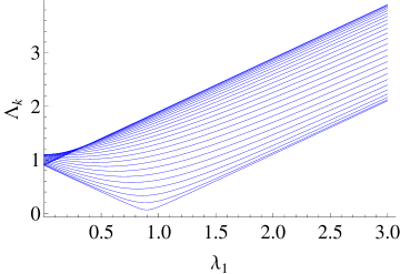
Figure 1: (color online) Plot of the single-fermion energy levels $\Lambda_{k}$ [Eq. (12)] as a function of $\lambda_{1}$ for $N=51$, $\lambda_{2}=0.1$ and $k$ ranging from 0 to $\pm$ 25. The lowest graph represents $k=\pm 25$. From top to bottom (on the right hand side of the plot) the graphs are ordered from lowest ($k=0$) to highest ranging ($k=\pm 25$) values.

The minimum gap $\Delta_{\rm eg,min}(M)$ is thus inversely proportional to the number of qubits murg2 , irrespective of the number of nearest-neighbour interactions $M$. From Eq. (17) we obtain that adding beyond-nearest-neighbour interactions increases the minimum gap by

$$\Delta_{\rm eg,min}(M)-\Delta_{\rm eg,min}(M-1) = \frac{\pi\Gamma}{N}\,\left(1-\sum_{j=1}^{M-1}\lambda_{j}\right)$$ (18)

$$= \frac{\pi\Gamma\lambda_{M}}{N}>0.$$

In Fig. 1 the energy levels for the single-fermion excited states (12) are plotted as a function of $\lambda_{1}$ for fixed $\lambda_{2}$. The minimum gap indeed occurs for $\lambda_{1}+\lambda_{2}=1$.

IV.2 Perturbation theory in the longitudinal field

We now apply perturbation theory to calculate the effect of the longitudinal field $h_{i}$ [the third term in Eq. (6) which we denote by $H_{3}$] on the level spectrum (13). In terms of the fermionic operators $\eta_{k}^{\dagger}$ and $\eta_{k}$ in Eq. (10), $H_{3}$ is written as:

$$\frac{H_{3}}{\Gamma} = -\sum_{i=1}^{N}\frac{h_{i}}{2\Gamma}(-1)^{N_{f}}\left(c_{i}^{\dagger}+c_{i}\right)$$ (19)

$$= -\sum_{k}r_{k}\left(\eta_{k}^{\dagger}+\eta_{k}\right),$$

with

$$r_{k}\equiv\sum_{i=1}^{N}\frac{h_{i}}{2\Gamma}(-1)^{N_{f}}\phi^{-1}_{ik},$$ (20)

$N_{f}$ the total number of $c$-fermions and $\phi^{-1}_{ik}$ given by Eq. (26). We denote the vacuum state by $|0\rangle$ and the state with one $\eta$-fermion by $|\theta_{p}\rangle$. For more $\eta$ fermions we use more indices, for example $|\theta_{p,q,r}\rangle$. To first order in $h_{i}$, the correction of the energy of the vacuum state is given by

$$\delta E_{0}^{(1)}=\left\langle 0\left|H_{3}\right|0\right\rangle\;\;=\;\;0.$$ (21)

Analogously, the first-order correction of the energy corresponding to state $|\theta_{m}\rangle$ is given by ovch03 :

$$\delta E_{m}^{(1)} = \left\langle\theta_{m}\left|H_{3}\right|\theta_{m}\right\rangle$$

$$= -\Gamma\langle\theta_{m}|\sum_{k}r_{k}\left(\eta_{k}^{\dagger}+\eta_{k}\right)|\theta_{m}\rangle$$

$$= -\Gamma\left(\sum_{k\neq m}r_{k}\langle\theta_{m}|\theta_{k,m}\rangle+r_{m}\langle\theta_{m}|0\rangle\right)$$

$$= 0.$$

This line of reasoning can be extended to all odd-order corrections of the energy levels, see Appendix A. The lowest nonzero correction to the energy spectrum is thus the second-order correction. For the ground state $|0\rangle$ this is given by:

$$\delta E_{0}^{(2)} = \Gamma^{2}\sum_{k}\frac{\bigg{|}\langle 0|\sum_{l}r_{l}\left(\eta_{l}^{\dagger}+\eta_{l}\right)|\theta_{k}\rangle\bigg{|}^{2}}{E_{0}-E_{k}}$$ (22)

$$= -\Gamma\sum_{k}\frac{r_{k}^{2}}{\Lambda_{k}}.$$

To second order the corrections to the energies of the single fermion states $|\theta_{m}\rangle$ are given by:

$$\delta E_{m}^{(2)} = \Gamma^{2}\left[\frac{|\langle\theta_{m}|r_{m}\eta_{m}^{\dagger}|0\rangle|^{2}}{E_{m}-E_{0}}+\sum_{k\neq m}\frac{|\langle\theta_{m}|r_{k}\eta_{k}|\theta_{m,k}\rangle|^{2}}{E_{m}-E_{mk}}\right]$$ (23)

$$= \Gamma\left[2\frac{r_{m}^{2}}{\Lambda_{m}}-\sum_{k}\left(\frac{r_{k}^{2}}{\Lambda_{k}}\right)\right].$$

Higher-order corrections and a discussion of the validity of perturbation theory are given in Appendix A. For a site-independent longitudinal field $h_{i}\equiv h\;\forall i$ we obtain from Eq. (20):

$$r_{k} = \begin{cases}\begin{array}[]{lll}\frac{h}{2\Gamma}\sqrt{\frac{2}{N}}\tan\left(\frac{k\pi}{N}\right)&\textrm{for}&k>0\\ \frac{h}{4\Gamma}\sqrt{\frac{2}{N}}&\textrm{for}&k=0\\ \frac{h}{2\Gamma}\sqrt{\frac{2}{N}}&\textrm{for}&k<0\end{array}\end{cases}$$ (24)

Here we have used the inverse of the functions $\phi_{ki}$ and $\psi_{ki}$ [Eqns. (11)], that are defined by

$$\sum_{k}\phi^{-1}_{ik}\phi_{ki}=\sum_{k}\psi^{-1}_{ik}\psi_{ki}=1\;\;\forall i,$$ (25)

and are given by (for arbitrary $N$)

$$\phi^{-1}_{ik} = \left(1-\frac{1}{2}\delta_{0k}-\frac{1}{2}\delta_{\frac{N}{2}k}\right)\phi_{ki}$$

$$\psi^{-1}_{ik} = -\left[1+\lambda_{1}\cos\left(\frac{2\pi k}{N}\right)-\lambda_{2}\cos\left(\frac{4\pi k}{N}\right)\right]\frac{\phi^{-1}_{ik}}{\Lambda_{k}}$$ (26)

$$-\left[\lambda_{1}\sin\left(\frac{2\pi k}{N}\right)-\lambda_{2}\sin\left(\frac{4\pi k}{N}\right)\right]\frac{\phi^{-1}_{i(-k)}}{\Lambda_{k}}\;\;\;$$

Finally, we note that Eq. (20) can also be used to calculate $r_{k}$ if the longitudinal field is site-dependent. For example, if $h_{i}$ has a given statistical distribution, Eq. (20) can be used to calculate the corresponding distribution and average of $r_{k}$.

IV.3 Scaling behavior of the gap

Using Eqns. (22) and (23) we now investigate the second-order correction of the gap $\delta\Delta_{eg,m}^{(2)}$ between the ground state and the $m^{th}$ single-fermion state:

$$\delta\Delta_{{\rm eg},m}^{(2)} \equiv \delta E_{m}^{(2)}-\delta E_{0}^{(2)}$$ (30)

$$= 2\,\Gamma\frac{r_{m}^{2}}{\Lambda_{m}}$$

$$= \frac{h^{2}}{\Gamma N}\left\{\begin{array}[]{ll}\frac{\tan^{2}\left(\frac{m\pi}{N}\right)}{\Lambda_{m}}&m>0\\ \frac{1}{4\Lambda_{0}}&m=0.\\ \frac{1}{\Lambda_{m}}&m<0\end{array}\right.$$

From Sec. IV.1 we know that the minimum gap in the absence of the longitudinal field occurs for $m=\pm\frac{N-1}{2}$ and $\sum_{j=1}^{M}\lambda_{j}=1$. The longitudinal field lifts the degenracy of the $\pm(\frac{N-1}{2}$)-fermion levels. Using Eq. (30) we then obtain for the corresponding corrections of the gap (at $\sum_{j=1}^{M}\lambda_{j}=1$):

$$\delta\Delta_{{\rm eg},\frac{N-1}{2}}^{(2)} = \frac{h^{2}}{\Gamma N}\,\frac{\tan^{2}\left(\frac{\pi}{2}-\frac{\pi}{2N}\right)}{\Lambda_{\frac{N-1}{2}}}$$ (31a)

$$\approx \frac{4h^{2}N}{\pi\Gamma}\,\frac{1}{\Lambda_{\frac{N-1}{2}}}$$

$$\delta\Delta_{{\rm eg},-\frac{N-1}{2}}^{(2)} = \frac{h^{2}}{\Gamma N}\,\frac{1}{\Lambda_{\frac{N-1}{2}}}<\delta\Delta_{{\rm eg},\frac{N-1}{2}}^{(2)}.$$

Substituting Eq. (13) for $k=\frac{N-1}{2}$ into Eq. (LABEL:corrmingap), the second-order correction to the minimum gap is thus given by:

$$\delta\Delta_{\rm eg,min}^{(2)}(M)=\frac{h^{2}}{\pi\Gamma}\,\frac{1}{\sum_{j=1}^{M}j\lambda_{j}}.$$ (32)

Combining Eqns. (17) and (32) we then obtain for the minimum gap, up to second order in the longitudinal field $h$,

$$\Delta_{\rm eg,min}(M)=\frac{\pi\Gamma}{N}\sum_{j=1}^{M}j\lambda_{j}+\frac{h^{2}}{\pi\Gamma}\,\frac{1}{\sum_{j=1}^{M}j\lambda_{j}},$$ (33)

with $\sum_{j=1}^{M}\lambda_{j}=1$. Eq. (33) is the main result of our paper. We see that the presence of the longitudinal field leads to an increase of the gap by a factor that is independent of the number of qubits $N$. Although the $h$-dependent correction term Eq. (32) decreases when adding beyond-nearest-neighbour interactions (scaling as $\delta\Delta^{(2)}_{\rm eg,min}(M)-\delta\Delta^{(2)}_{\rm eg,min}(M-1)\sim-h^{2}\lambda_{M}/(\pi\Gamma)<0$) the minimum gap itself increases with $M$ since the first, unperturbed, term increases with $\lambda_{M}$.

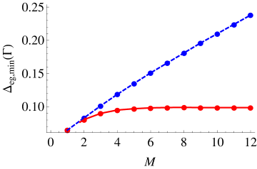
Figure 2: (color online) Plot of the minimum gap $\Delta_{\rm eg,min}$ [Eq. (33)] in units of $\Gamma$ as a function of $M$ for $h/\Gamma=0.1$ and $N=51$. The blue dashed line represents linear ($\lambda_{j}=\textrm{const}/j$) and the red solid line represents exponential ($\lambda_{j}=\textrm{const}\cdot\exp{(-j)}$) decay of the interaction strength with distance between the bits. The constant is determined by the condition $\sum_{j=1}^{M}\lambda_{j}=1$.

Fig. 2 depicts $\Delta_{eg,min}$ in units of $\Gamma$ as a function of the number of neighbouring interactions $M$. We consider both interactions which decay linearly as a function of the distance between two qubits along the chain and interactions which decay exponentially. For both types of decay (although more strongly for linear than exponential decay) the minimum gap is enhanced by including coupling with more neighbours. Since the required running time of an adiabatic algorithm is inversely proportional to the square of the energy gap murg04 , the enhancement of the gap implies that a qubit system with beyond-nearest-neighbour interactions may be advantageous for implementing adiabatic quantum algorithms.

V Relation to Exact Cover 3

In this section we investigate how the extended quantum Ising model from the previous section with uniform beyond-nearest-neighbour interactions can be used to simulate specific instances of Exact Cover 3. In particular, we numerically estimate the probability for obtaining the correct solution of instances of Exact Cover 3 that are characterized by a maximum distance between bits in a clause as a function of the number $M$ of beyond-nearest-neighbour interactions that are included. At the end of the section we make a connection to an actual experimental system (a chain of flux qubits).

We consider a system of $N$ bits with coupling to $M$ nearest neighbours. Since each bit is coupled to $M$ bits on either side, the maximum distance between two bits that appear in the same clause is $2M$ (see also Eq. (3)). Out of the set of all possible clauses, we restrict ourselves to clauses that satisfy this property, i.e. contain bits which are at most a distance $2M$ along the chain apart. We refer to this subset as the set of ”restricted clauses”. Clauses in which no maximum distance between the bits is defined, are called ”unrestricted clauses”. For clauses $\{\alpha,\beta,\gamma\}$ with $\alpha<\beta<\gamma$ we only allow restricted clauses that satisfy $\gamma-\alpha\leq 2M$ or $(\alpha+N)-\beta\leq 2M$ or $(\beta+N)-\gamma\leq 2M$ and in order to avoid boundary effects we consider a cyclic chain of bits. The question that we raise is the following: what is the probability that a particular solution of Exact Cover 3, represented by a random bit chain (in which each bit independently has a probability $p$ for taking value $1$) can be reconstructed using $K$ restricted clauses? In our simulations the restricted clauses for given $K$ are selected from a large group of unrestricted clauses that are uniformly distributed over the $N$ bits in the qubit chain meza02 . For some limits the answer to this question is obvious: in particular, for $p$ close to $0$ or $1$ there are too many bits with the same value, and no restricted set of clauses, or indeed unrestricted set of clauses, can be found that gives a uniquely satisfying assignment.

We now describe our simulations. For specific values of $N$, $M$, $p$, and $K$ we generate $100$ random bit strings bitstrings . For each of these we randomly generate $500$ clauses (or more if needed) that are satisfied by the given bit string. Out of these we randomly select $K$ clauses that satisfy the $M$-nearest-neighbour restriction condition. Then we check whether the original bit string is the unique solution of the restricted set of clauses. If each bit is covered by at least one clause, the solution is usually unique. Out of $100$ runs we deduce a probability $p_{E}$ that an error will occur, meaning that at least one other bit string also satisfies the assignment of $K$ clauses. Our goal is to determine at which point $p_{E}$ makes a transition from large ($p_{E}\approx 1$) to small ($p_{E}\approx 0$) as a function of the parameters $p$ and $M$. In the table below, we keep $N$ and $K$ fixed at $N=12$ and $K=20$, and calculate $p_{E}$ as a function of $K$ for various probabilities $p$. The ratio $K/N$ is chosen large enough that once the bits allow a uniquely satisfying assignment of restricted clauses for a given $p$, this is also formed in the simulations with high probability.

$M$	1	2	3	4	5	6	7	8
$p_{E}$ for $p=0.2$	1.00	0.64	0.36	0.22	0.14	0.14	0.10	0.09
$p_{E}$ for $p=0.3$	1.00	0.43	0.22	0.11	0.10	0.10	0.09	0.05
$p_{E}$ for $p=0.4$	1.00	0.51	0.26	0.18	0.16	0.10	0.10	0.09
$p_{E}$ for $p=0.5$	1.00	0.67	0.34	0.23	0.22	0.18	0.17	0.13

Table 1: The probability $p_{E}$ for errors to occur as a function of the number $M$ of beyond-nearest-neighbour interactions for $p=0.2,0.3,0.4,$ and $0.5$.

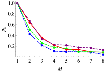
Figure 3: (color online) The probability $p_{E}$ from Table 1 as a function of $M$ for $p=0.2$ (red, solid), $p=0.3$ (blue, dot-dashed), $p=0.4$ (green, dashed), and $p=0.5$ (purple, dotted).

From Table 1 we see that for all values of $p$ a transition from large to small error probability takes places for $M$ ranging from $1$ to $8$. For $p=0.3$ the probability of errors to occur for a given value of $M$ is smallest, which can be explained from the optimal ratio of bitvalues $0$ and $1$ for finding clauses. Fig. 3 shows a graphic representation of Table 1. We see that the probability for an error to occur during simulation of restricted instances of Exact Cover 3 decreases approximately exponentially with increasing $M$.

Our simulations did not take into account the fact that the interaction strength $\lambda_{n}$ between qubits $i$ and $i+n$ - which translates into the number of clauses that contain both bit $i$ and bit $i+n$, see Eq. (3) - in practice decreases as a function of the distance $n$ between the qubits. In order to make a connection to the Exact Cover Hamiltonian (3) we in principle thus need to further restrict the sets of ”restricted clauses” to sets in which the number of clauses containing nearby qubits is larger than the number of clauses containing bits that are farther apart. Although we did not investigate this in depth, back-of-the-envelope estimates indicate that in order to reach the same success probability a factor of $2$ more clauses need to be included in the simulations.

In order to simulate Exact Cover 3 in practice, one needs to use adiabatic evolution of the Hamiltonian (4), whose final ground state at time $T$ encodes the solution of the Exact Cover problem. In their general form, the Hamiltonians (4) and (7) are still far from experimental realization. The closest analogy between (4) and an actual experimental qubit system is probably a chain of coupled flux qubits, which can be described by the Hamiltonian maje05 ; dica09

$$H_{\rm fluxchain}=\sum_{i=1}^{N}\Delta_{i}\sigma_{x}^{i}+\sum_{i=1}^{N}K_{i,i+1}\sigma_{z}^{i}\sigma_{z}^{i+1}+\sum_{i=1}^{N}\epsilon_{i}\sigma_{z}^{i}.$$ (34)

Here $\epsilon_{i}$ denotes the magnetic energy, $\Delta_{i}$ the tunnel coupling energy of individual qubits and $K_{i,i+1}\sim M_{i,i+1}I_{p}^{i}I_{p}^{i+1}$ with $M_{i,i+1}$ the mutual inductance between the persistent currents $I_{p}^{i}$ and $I_{p}^{i+1}$ of qubits $i$ and $i+1$, respectively. In practice, local (in situ) tuning of the parameters $\Delta_{i}$, $K_{i,i+1}$ and $\epsilon_{i}$, as required by adiabatic evolution of Eq. (4), is challenging, but promising progress is being made paau09 ; dica09 . This gives hope for achieving control over individual qubits in chain and array-like qubit geometries and thereby brings experimental simulation of adiabatic quantum algorithms such as Exact Cover 3 closer.

VI Conclusion

In conclusion, we have calculated the energy level spectrum of the quantum Ising model in the presence of uniform beyond-nearest-neighbour interactions and an additional longitudinal field. We found that the gap between the ground state and the lowest-lying excited state increases with increasing number $M$ of neighbouring interactions (provided $M$ remains much smaller than the total number of qubits along the chain) and is approximately linearly proportional to $M$ for linearly decreasing interaction strength between the qubits along the chain. The increase of this gap with $M$, which persists in the presence of the additional weak longitudinal field, gives hope that the extended quantum Ising model is suitable for numerical - and in the future hopefully also experimental - simulation of quantum algorithms such as Exact Cover 3.

Appendix A

In this Appendix we investigate the validity of the perturbative approach that we used in Sec. IV.2 and derive a criterion for the application of perturbation theory in terms of the number of qubits ($N$) and the number of nearest neighbours included ($M$). We first demonstrate that all odd-order corrections to the single-fermion energy levels are zero and then investigate even-order corrections. Our starting point is the third-order correction, which in general form is given by:

$$\delta E_{p}^{(3)} = \sum_{q\neq p}\sum_{r\neq p}\frac{\langle\theta_{p}|H_{3}|\theta_{q}\rangle\langle\theta_{q}|H_{3}|\theta_{r}\rangle\langle\theta_{r}|H_{3}|\theta_{p}\rangle}{\left(E_{p}-E_{q}\right)\left(E_{p}-E_{r}\right)}$$ (35)

$$-\langle\theta_{p}|H_{3}|\theta_{p}\rangle\sum_{q\neq p}\frac{|\langle\theta_{p}|H_{3}|\theta_{q}\rangle|^{2}}{\left(E_{p}-E_{q}\right)^{2}}.$$

It can be seen immediately that the second term is zero since it contains the matrix element $\langle\theta_{p}|H_{3}|\theta_{p}\rangle$, which is zero (see Eq. (IV.2)). The first term in Eq. (35) contains three separate matrix elements. Let us assume that in the first product $\theta_{p}$ is an even-fermion state, which is then coupled to odd-fermion states $\theta_{q}$ by $H_{3}$. This in turn restricts $\theta_{r}$ to the even fermion subspace. Applying the same reasoning to the last inner product we see that for this product to be non-zero $\theta_{p}$ should be an odd-fermion state. This is a contradiction with our starting assumption. Hence there is no combination of states that gives a non-zero outcome. This observation can be extended to all odd-order energy corrections and we conclude that these are therefore all zero ovch03 .

We now investigate even-order corrections to the energy of the ground state and single-fermion states and use these to derive a criterion for the validity of perturbation theory. Our starting point is the second-order correction of the ground state, which can be found by inserting Eqns. (13) and (24) into Eq. (22). This yields:

$$\delta E_{0}^{(2)}=-\frac{h^{2}}{2N\Gamma}\left[\frac{1}{4\Lambda_{0}}+\sum_{k=1}^{(N-1)/2}\left(\frac{1+\tan^{2}\left(\frac{\pi k}{N}\right)}{\Lambda_{k}}\right)\right].$$ (36)

After defining $\tilde{M}\equiv\sum_{j=1}^{M}j\lambda_{j}$, rewriting the sum using $m=N-2k$ and expanding around $m=0$ (which yields the largest contribution to the sum), Eq. (36) reduces to

$$\delta E_{0}^{(2)} \approx \frac{h^{2}}{2N\Gamma}\sum_{\begin{subarray}{c}m=1\\ m\;\textrm{odd}\end{subarray}}^{N-1}\frac{1+\left(\frac{2N}{m\pi}\right)^{2}}{\tilde{M}\left(\frac{m\pi}{N}\right)}$$ (37)

$$\approx -0.068\,\frac{h^{2}N^{2}}{\Gamma\tilde{M}}.$$

Analogously we obtain for the fourth-order correction:

$$\delta E_{0}^{(4)} = \Gamma\sum_{k,l}\left(\frac{r_{k}}{2}\right)^{2}\left(\frac{r_{l}}{2}\right)^{2}\left[\Lambda_{k}^{2}\left(\Lambda_{k}+\Lambda_{l}\right)\right]^{-1}$$ (38)

$$\approx \frac{4}{\pi^{5}}\,\frac{h^{4}N^{5}}{(\Gamma\tilde{M})^{3}}\sum_{\begin{subarray}{c}m=1\\ m\;\textrm{odd}\end{subarray}}^{N-1}\sum_{\begin{subarray}{c}n=1\\ n\;\textrm{odd}\end{subarray}}^{N-1}\frac{m^{-4}n^{-2}}{m+n}$$

$$\approx 0.0071\,\frac{h^{4}N^{5}}{(\Gamma\tilde{M})^{3}}.$$

We are interested in the energy gap between the ground state and the first excited states ($N-2k\ll N$), which in the absence of the longitudinal field $h$ is given by

$$\Delta_{eg,k}\equiv E_{k}^{(0)}-E_{0}^{(0)}=\Gamma\Lambda_{k}=\frac{\pi}{N}\Gamma\tilde{M}(N-2k),$$ (39)

and reduces to Eq. (17) for the lowest-lying excited state (given by $k=(N-1)/2$). The second-order corrections to this gap between the ground state and the lowest-lying excited states ($N-2k\ll N$) are given by (see Eq. (30))

$$\delta E_{k}^{(2)}-\delta E_{0}^{(2)}=2\Gamma\frac{(r_{k})^{2}}{\Lambda_{k}}=\frac{4}{\pi^{3}}\frac{h^{2}}{\Gamma}\frac{N^{2}}{\tilde{M}(N-2k)}.$$ (40)

For the general $(2n)^{th}$-order correction to the gap we find

$$\delta E_{k}^{(2n)}-\delta E_{0}^{(2n)}\propto\frac{h^{2n}N^{3n-1}}{(\Gamma\tilde{M})^{2n-1}}.$$ (41)

It follows from Eq. (41) that perturbation theory is valid for

$$\frac{h}{\Gamma}\ll\frac{\tilde{M}}{N^{3/2}}.$$ (42)

Fig. 2 in the main text shows a plot of $\Delta_{eg,min}$, which is directly proportional to $\tilde{M}$, as a function of the number of neighbouring interactions $M$. For exponential decay the value of $\tilde{M}$ converges for $M$ large (but still much smaller than $N$), but for linear coupling $\tilde{M}$ scales almost linear with $M$. For a given number of qubits $N$ and linear decay of interaction strength along the chain adding more nearest-neighbours thus enhances the range of validity of perturbation theory.

References

- (1) P.W. Shor, SIAM J. Comput. 26, 1484 (1997); L.K. Grover, Phys. Rev. Lett. 79, 325 (1997); see also M.A. Nielsen and I.L. Chuang, Quantum Computation and Quantum Information, (Cambridge University Press, Cambridge, 2000).
- (2) R. Hanson, L.P Kouwenhoven, J.R. Petta, S. Tarucha, and L.M.K. Vandersypen, Rev. Mod. Phys. 79, 1217 (2007).
- (3) G. Wendin and V.S. Shumeiko, in Handbook of Theoretical and Computational Nanotechnology, Vol. 3, Ed. M. Rieth and W. Schommers, (American Scientific Publishers, Los Angeles, 2006); See also ArXiv:cond-mat/0508729
- (4) E. Farhi, J. Goldstone, S. Gutmann, J. Lapan, A. Lundgren, and D. Preda, Science 292, 472 (2001).
- (5) NP stands for non-polynomial, see for example the book by Nielsen and Chuang shor97 for further explanation.
- (6) V. Murg and J.I. Cirac, Phys. Rev. A 69, 042320 (2004).
- (7) M.H.S. Amin, Phys. Rev. Lett. 100, 130503 (2008).
- (8) A.M. Childs, E. Farhi and J. Preskill, Phys. Rev. A 65, 012322 (2001); M.S. Sarandy and D.A. Lidar, Phys. Rev. Lett. 95, 250503 (2005); J. Roland and N.J. Cerf, Phys. Rev. A 71, 032330 (2005); S. Ashhab, J.R. Johansson, and F. Nori, ibid. 74, 052330 (2006); M. Tiersch and R. Schützhold, ibid. 75, 062313 (2007).
- (9) M.H.S. Amin, P.J. Love and C.J.S. Truncik, Phys. Rev. Lett. 100, 060503 (2008); M.H.S. Amin, D.V. Averin, and J.A. Nesteroff, Phys. Rev. A 79, 022107 (2009); M.H.S. Amin, C.J.S. Truncik, and D.V. Averin, ibid. 80, 022303 (2009).
- (10) S. Lloyd, ArXiv:0805.2757.
- (11) R. Schützhold and G. Schaller, Phys. Rev. A 74, 060304(R) (2006).
- (12) M.H.S. Amin and V. Choi, Phys. Rev. A 80, 062326 (2009).
- (13) B. Altshuler, H. Krovi and J. Roland, Proc. Natl. Acad. Sci. 107, 12446 (2010).
- (14) A.P. Young, S. Knysh and V.N. Smelyanskiy, Phys. Rev. Lett. 101, 170503 (2008); A.P. Young, S. Knysh, and V.N. Smelyanskiy, ibid. 104, 020502 (2010); I. Hen and A.P. Young, ArXiv:1109.6872.
- (15) V. Choi, Proc. Natl. Acad. Sci. 108, E19 (2011); See also the discussion and overview by N.G. Dickson and M.H.S. Amin, Phys. Rev. Lett. 106, 050502 (2011).
- (16) E. Lieb, T. Schultz, and D. Mattis, Ann. Phys. 16, 407 (1961).
- (17) See e.g. the flux qubit chains described in F.G. Paauw, PhD Thesis (Delft University of Technology, 2009); J.B. Majer, F.G. Paauw, A.C.J. ter Haar, C.J.P.M Harmans, and J.E. Mooij, Phys. Rev. Lett. 94, 090501 (2005).
- (18) M.C. Bañuls, R. Orús, J.I. Latorre, A. Pérez, and P. Ruiz-Femenía, Phys. Rev. A 73, 022344 (2006).
- (19) A. Fubini, G. Falci, and Andreas Osterloh, New J. Phys. 9, 134 (2007).
- (20) A.A. Ovchinnikov, D.V. Dmitriev, V.Ya. Krivnov and V.O. Cheranovskii, Phys. Rev. B 68, 214406 (2003).
- (21) This corresponds to an exactly solvable spin-chain model commonly denoted as the XXZ model, see Ref. suzu71 . In practice, three-qubit interactions can in principle be realized for e.g. superconducting qubits by extending the cavity bus coupling method that was pioneered by Majer et al., Nature 449, 443 (2007).
- (22) S. Suzuki, Phys. Lett. A 34, 338 (1971); S. Suzuki, Prog. Theor. Phys. 46, 1337 (1971).
- (23) P. Pfeuty, Ann. Phys. 57, 79 (1970).
- (24) This is the generalization of the situation encountered for even and when only nearest neighbour coupling is included. murg04 ; pfeu70
- (25) This has been noted before for the quantum Ising model with nearest-neighbour interactions only, see e.g. Ref. murg04 .
- (26) For unrestricted clauses M. Mézard and R. Zecchina [Phys. Rev. E 66, 056126 (2002)] have calculated the critical values (with ) for which solutions of 3-satisfiability problems such as Exact Cover 3 become clustered, and for which solutions become unique. Although it is beyond the scope of this paper, it would be interesting to investigate the same question for the restricted clauses used in Sec. V.
- (27) We verified that adding more instances only changes in the 4 decimal (or smaller).
- (28) See e.g. L. DiCarlo et al., Nature 460, 240 (2009); R. Harris et al., Phys. Rev. B 82, 024511 (2010).
- (29) F.G. Paauw, A. Fedorov, C.J.P.M. Harmans, and J.E. Mooij, Phys. Rev. Lett. 102, 090501 (2009).