Entangling two distant nanocavities via a waveguide

Abstract

In this paper, we investigate the generation of continuous variable entanglement between two spatially-separate nanocavities mediated by a coupled resonator optical waveguide in photonic crystals. By solving the exact dynamics of the cavity system coupled to the waveguide, the entanglement and purity of the two-mode cavity state are discussed in detail for the initially separated squeezing inputs. It is found that the stable and pure entangled state of the two distant nanocavities can be achieved with the requirement of only a weak cavity-waveguide coupling when the cavities are resonant with the band center of the waveguide. The strong couplings between the cavities and the waveguide lead to the entanglement sudden death and sudden birth. When the frequencies of the cavities lie outside the band of the waveguide, the waveguide-induced cross frequency shift between the cavities can optimize the achievable entanglement. It is also shown that the entanglement can be easily manipulated through the changes of the cavity frequencies within the waveguide band.

I Introduction

Entanglement of electromagnetic field with continuous variables Braunstein1 , which embodies quantum correlations in amplitude and phase quadratures of the field, has been proven to be very important for building up continuous variable quantum communication network Braunstein3 ; jia ; Che09214538 ; shen and quantum computation oneway ; error ; gate . Generally, continuous variable entanglement is generated via nondegenerate optical parametric oscillation jia ; shen ; lett ; guman ; li or beam splitters incorporating with squeezed light beams Braunstein3 ; ch .

Based on recent achievements in the light manipulation with highly controllable photonic crystals notomi1 , we investigate in this paper the generation of continuous variable entanglement between two spatially-separated nanocavities mediated by a coupled-resonator optical waveguide (CROW) in photonic crystals. As we know, the long-distance entanglement is an essential ingredient for transmitting quantum information over long distances in quantum communication networks duan ; kimble . Very recently, the distant entanglement between two qubits mediated by a plasmic waveguide tudela or two vibrating trapped ions assisted by a phononic reservoir wolf has just been studied. Here we shall focus on the distant continuous variable entanglement between two nanocavity fields. The main merits of the present scheme are as follows. The nanocavity could be a point defect created in photonic crystals and its frequency can be simply controlled just by changing the size or the shape of the defect noda . While the waveguide, as the mediator of the two cavities as well as the output channel, can be considered as a set of linearly coupled defects in photonic crystals in which light propagates due to the coupling between the adjacent defects yariv ; notomi2 . The transmission properties of the CROW can also be easily manipulated by changing the modes of the resonators and the coupling configuration baba . Furthermore, the coupling of the cavity to the waveguide is also controllable through the change of the distance between the corresponding defects fan . Besides the above flexible controllability, the possibility of miniaturizing the entanglement setup with solid-state photonic structures is highly desirable for scalable and on-chip photonic quantum information processing brien ; linda . Obviously, the bulk setups for producing continuous variable entangled light in Refs.Braunstein3 ; jia ; shen ; oneway ; error ; gate ; lett ; guman ; li ; ch are not suitable for integration. In addition, compared to qubit or phononic entanglement proposed in Refs.tudela ; wolf , optical entanglement with continuous variables can be easily detected and manipulated experimentally, which can make it very promising for the implementation of continuous variable quantum protocols Braunstein3 ; jia ; Che09214538 ; shen ; oneway ; error ; gate .

The effects of various environments on continuous variable entanglement of optical fields or harmonic oscillators have been extensively investigated, where one is mainly interested in the non-Markovian decoherence dynamics of the entanglement bm1 ; An ; so2 ; so3 ; so4 . For the present system of two spatially-separated nanocavities mediated by a waveguide, the waveguide actually serves as a structured reservoir which is highly controllable in experiments. We therefore are interested in the entanglement generation and its manipulation through the controls of the waveguide as well as the nanocavity properties. We shall study the exact entanglement dynamics solved from the exact master equation of the nanocavity system coupled to the waveguides that we developed very recently xiong ; wu ; tan ; lei . The temporal behavior of the entanglement and purity of the two-mode cavity state is discussed in detail for initially separated squeezing inputs. We find that when the cavity frequencies are resonant with the band center of the waveguide, a stable and pure entangled state of the two distant cavities can be generated with a requirement of only a very weak coupling between the cavities and the waveguide. It shows that the strong cavity-waveguide coupling will lead to the entanglement sudden death and sudden birth yu . When the frequencies of the cavities locate outside the waveguide band, the cross frequency shift of the nanocavities induced by the waveguide can optimize the achievable entanglement. In addition, it is also shown that the entanglement can be easily manipulated by changing the cavity frequencies within the waveguide band.

The rest of the paper is organized as follows. In Sec. II, we formulate the entanglement dynamics of two spatially-separated nanocavities coupled to a waveguide within the framework of the exact master equation and the correlation matrix, the later determines the continuous variable entanglement of the two nanocavities through the measure of logarithmic negativity. In Sec. III, the properties of the entanglement and the corresponding purity are investigated in detail. Finally, a conclusion is given in Sec. IV.

II Hamiltonian and entanglement measure

Figure 1: A schematic plot of two spatially-separated nanocavities coupled to a CROW structure at the sites $n_{i}~{}(i=1,2)$ in photonic crystals.

As schematically shown in Fig. 1, we consider two single-mode nanocavities coupled with a coupled resonator optical waveguide (CROW) in photonic crystals at different sites. Each cavity is formed by a point defect created in photonic crystals, with the cavity frequency tunable by changing the geometrical parameters of the defect. The waveguide in photonic crystals consists of a series of coupled point defects in which light propagates due to the coupling between the adjacent defects. Experimentally, the large-scale CROW consisting of more than one hundred coupled resonators has been successfully fabricated noda . To be specific, let the cavity 1 be coupled to the waveguide at the site $n_{1}$ and the cavity 2 coupled to the waveguide at the site $n_{2}$, as shown in Fig. 1. By treating the waveguide as a tight-binding model, the Hamiltonian of the whole system is given by wu

$$H= \sum_{i=1,2}\omega_{i}a_{i}^{\dagger}a_{i}+\sum_{k}\omega_{k}b_{k}^{\dagger}b_{k}+\sum_{i,k}V_{ik}(a_{i}b_{k}^{\dagger}+b_{k}a_{i}^{\dagger}),$$ (1)

where

$$\omega_{k}=\omega_{0}-2\xi_{0}\cos k,\ ~{}~{}V_{ik}=\sqrt{\frac{2}{\pi}}\xi_{i}\sin(n_{i}k),$$ (2)

with $0\leq k\leq\pi$. The operators $a_{i}$ and $a_{i}^{\dagger}$ are the annihilation and creation operators of the cavity fields with frequencies $\omega_{i}$. The annihilation and creation operators $b_{k}$ and $b_{k}^{\dagger}$ describe the Bloch modes $\omega_{k}$ of the waveguide with $\omega_{0}$ being the identical frequency of each resonator in the waveguide. The frequencies $\omega_{i}$ and $\omega_{0}$ are tunable by adjusting the geometrical parameters of the corresponding defects. The strength $\xi_{0}$ characterizes the photon hopping between two adjacent resonators in the waveguide and is controllable by changing the corresponding distance between the two defects. The controllable coupling strength $\xi_{i}$ is the coupling of the $i$th cavity to the waveguide at the sites $n_{i}$. We should point out that the frequencies of the two cavities and the waveguide band considered in the above system should lie inside the photonic band gap of the photonic crystals. Then the photon loss into the photonic crystals is totally negligible Notomi .

We will investigate the generation of the entanglement between the two spatially-separated cavity fields through the controllable waveguide, where the two nanocavities are initially prepared in a separated two-mode Gaussian state. For a two-mode Gaussian state, its quantum statistical property is fully determined by the $4\times 4$ correlation matrix $\bm{\chi}$ which is defined by

$$\chi_{ij}=\frac{1}{2}\langle x_{i}x_{j}+x_{j}x_{i}\rangle,$$ (3)

where the vector $x=(X_{1},Y_{1},X_{2},Y_{2})$ and the quadrature operators $X_{j}=(a_{j}+a_{j}^{\dagger})/\sqrt{2}$ and $Y_{j}=-i(a_{j}-a_{j}^{\dagger})/\sqrt{2}$. With the correlation matrix $\bm{\chi}$, the continuous variable entanglement between the two cavity fields can be well quantified with the measure of logarithmic negativity. By re-expressing the correlation matrix $\bm{\chi}$ in terms of three $2\times 2$ matrices $\bm{\varrho}_{1}$, $\bm{\varrho}_{2}$, and $\bm{\varrho}_{3}$,

$$\bm{\chi}=\begin{pmatrix}\bm{\varrho}_{1}&\bm{\varrho}_{3}\\ \bm{\varrho}_{3}^{T}&\bm{\varrho}_{2}\end{pmatrix},$$ (4)

the logarithmic negativity $E_{N}(\bm{\chi})$ is defined as vidal

$$E_{N}(\bm{\chi})=\textrm{max}[0,-\textrm{ln}(2\lambda)],$$ (5)

where

$$\lambda=\frac{\sqrt{\Delta-\sqrt{\Delta^{2}-4~{}\textrm{Det}\bm{\chi}}}}{\sqrt{2}},$$ (6)

and $\Delta=\textrm{Det}\bm{\varrho}_{1}+\textrm{Det}\bm{\varrho}_{2}-2~{}\textrm{Det}\bm{\varrho}_{3}$. Thus, the entanglement between the two cavity fields occurs for $E_{N}(\bm{\chi})>0$, i.e., for $\lambda>\frac{1}{2}$. From the definitions of Eqs. (3) and (4), we see that the matrix elements of $\bm{\chi}$ are a linear function of the second-order quantities

$$n_{ij}(t)=\langle a^{\dagger}_{i}(t)a_{j}(t)\rangle,~{}~{}s_{ij}(t)=\langle a_{i}(t)a_{j}(t)\rangle$$ (7)

plus its hermitian conjugate. The entanglement dynamics between the two cavity fields at any time is then completely determined by these time-dependent second-order quantities.

On the other hand, the Hamiltonian of Eq. (1) describes effectively the two spatially-separated nanocavities coupled to a common reservoir with a controllable spectral structure. In other words, the waveguide plays a role of a structured reservoir as a mediator between two nanocavities. We can use the exact master equation we developed recently for nanocavities coupled to waveguides in photonic crystals wu ; tan ; lei to investigate the exact entanglement dynamics of the two nanocavities coupled to the waveguide in photonic crystals. By assuming that two nanocavities are initially uncorrelated to the structured reservoir (i.e., the waveguide) and the waveguide is initially in vacuum, the exact master equation for the density operator $\rho(t)$ of the cavity system can be obtained through the Feynman-Vernon influence functional approach Fey in the framework of coherent state path-integral representation Zhang2 . The resulting exact master equation is given by

$$\frac{d\rho(t)}{dt}=-i[H_{\textrm{eff}}(t),\rho(t)]$$

$$~{}~{}+\sum_{ij}\gamma_{ij}(t)[2a_{j}\rho(t)a_{i}^{\dagger}-a_{i}^{\dagger}a_{j}\rho(t)-\rho(t)a_{i}^{\dagger}a_{j}],$$ (8)

where $H_{\textrm{eff}}(t)=\omega_{ij}(t)a_{i}^{\dagger}a_{j}$ is the effective Hamiltonian of the cavity fields with the time-dependent renormalized frequencies $\omega_{ij}(t)$, which is resulted from the back-reaction of the the waveguide to the cavity system. The time-dependent coefficients $\bm{\gamma}(t)$ describe the dissipation of the cavity system due to the coupling to the waveguide. The coefficients $\omega_{ij}(t)$ and $\bm{\gamma}(t)$ are non-perturbatively determined by

$$\omega_{ij}(t) =\frac{i}{2}[\dot{\bm{\mu}}(t)\bm{\mu}^{-1}(t)-h.c.]_{ij},$$ (9a)

$$\gamma_{ij}(t) =-\frac{1}{2}[\dot{\bm{\mu}}(t)\bm{\mu}^{-1}(t)+h.c.]_{ij},$$ (9b)

where $\bm{\mu}(t)$ is the cavity photon propagating function which obeys the integrodifferential equation of motion

$$\frac{d}{dt}\bm{\mu}(t)=-i\bar{\bm{\omega}}\bm{\mu}(t)-\int_{t_{0}}^{t}\bm{g}(t-\tau)\bm{\mu}(\tau)d\tau,$$ (10)

with the initial condition $\bm{\mu}(t_{0})=1$. Here, the frequency matrix $\bar{\bm{\omega}}=\textrm{Diag}[\omega_{1},\omega_{2}]$ is a diagonal frequency matrix of the two cavities. The integral kernel in Eq.(10) involves the time-correlation function $\bm{g}(\tau-\tau^{\prime})$, which non-perturbatively characterizes the non-Markovian memory structure between the cavity system and the waveguide.

By introducing the spectral densities of the waveguide: $J_{ij}(\omega)=2\pi\sum_{k}V_{ik}V_{jk}\delta(\omega-\omega_{k})$, the time-correlation function can be expressed as

$$g_{ij}(\tau-\tau^{\prime}) =\int\frac{d\omega}{2\pi}J_{ij}(\omega)e^{-i\omega(\tau-\tau^{\prime})}.$$ (11a)

Since the waveguide in photonic crystals has a narrow but continuous band structure, the spectral densities becomes $J_{ij}(\omega)=2\pi\varrho(\omega)V_{i}(\omega)V_{j}(\omega)$, where $\varrho(\omega)$ is the density of states in the waveguide determined by Eq. (2). Explicitly, we have

$$\varrho(\omega)=\frac{1}{\sqrt{4\xi_{0}^{2}-(\omega-\omega_{0})^{2}}},$$ (12a)

$$V_{i}(\omega)=\sqrt{\frac{2}{\pi}} \xi_{i}\sin[n_{i}\arcsin(\frac{\sqrt{4\xi_{0}^{2}-(\omega-\omega_{0})^{2}}}{2\xi_{0}})],$$ (12b)

where $\omega_{0}-2\xi_{0}\leq\omega\leq\omega_{0}+2\xi_{0}$ is the band of the waveguide. In Fig. 2, the spectral densities $J_{11}(\omega)=J_{22}(\omega)$ and $J_{12}(\omega)=J_{21}(\omega)$ are plotted as a function of $\omega$ with different distances between the two cavities, for the case of the equal cavity frequencies $\omega_{1}=\omega_{2}=\omega_{c}$ and the equal cavity-waveguide couplings $\xi_{1}=\xi_{2}=\xi_{c}$. As we will show later in the next section, the entanglement characteristics depend heavily on the spectral structures.

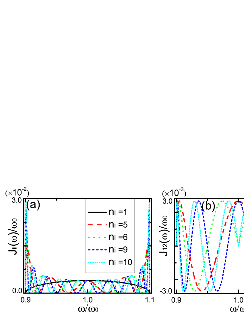
Figure 2: (a) The spectral density $J_{ii}(\omega)$ for the cavities at different locations $n_{i}$. (b) The spectral density $J_{12}(\omega)$ for the different sites $n_{2}$ of the second cavity and the first cavity location $n_{1}=1$. Here the two cavity frequencies are taken to be equal and also equal to the resonator frequency in the waveguides: $\omega_{1}=\omega_{2}=\omega_{0}$. The cavity-waveguide coupling $\xi_{1}=\xi_{2}=0.2\xi_{0}$, and the hopping rate in the waveguide $\xi_{0}=0.05\omega_{0}$.

In fact, it is the back-action through the off-diagonal matrix element $J_{12}(\omega)$ of the spectral density that induces an effective coupling between the two separated nanocavities which leads to the entanglement generation. The environment-assisted continuous variable entanglement has been investigated in the literature so2 ; s1 ; s2 . However, the entanglement in these investigations is uncontrollable. Here, the waveguide (a structured reservoir)-induced entanglement between two spatially-separated nanocavities in photonic crystals is fully controllable and is promising for quantum information processing in all-optical circuits.

Now, the exact temporal behavior of the second-order quantities of Eq. (7) can be completely determined by the exact master equation. Explicitly, from the exact master equation (8), it is not too difficult to find that the second-order quantities obey the following equations

$$\frac{d}{dt}\bm{n}(t) =[\dot{\bm{\mu}}(t)\bm{\mu}^{-1}(t)]\bm{n}(t)+\bm{n}(t)[\dot{\bm{\mu}}(t)\bm{\mu}^{-1}(t)]^{\dagger},$$ (13a)

$$\frac{d}{dt}\bm{s}(t) =[\dot{\bm{\mu}}(t)\bm{\mu}^{-1}(t)]\bm{s}(t)+\bm{s}(t)[\dot{\bm{\mu}}(t)\bm{\mu}^{-1}(t)]^{T}.$$ (13b)

The exact solutions of the above equations are found to be

$$\bm{n}(t)=\bm{\mu}(t)\bm{n}(0)\bm{\mu}^{\dagger}(t)~{},~{}~{}\bm{s}(t)=\bm{\mu}(t)\bm{s}(0)\bm{\mu}^{T}(t),$$ (14)

where $\bm{n}(0)$ and $\bm{s}(0)$ are the initial second-order quantities. Thus, once the photon propagating function $\bm{\mu}(t)$ is solved from the integrodifferential equations of motion (10), the above exact solution allows us investigate the entanglement generation of the two separated nanocavities. Meantime, the temporal evolution of the entanglement measure subjected to the non-Markovian dissipation and fluctuation from the structured reservoir can be fully taken into account.

III Results and discussion

Now we are ready to investigate the entanglement generation between the two cavity fields and its temporal evolution for a given initially-separated state. We assume that the two cavity fields are initially prepared in a single-mode squeezed state, respectively, i.e.,

$$|\psi_{a_{i}}(0)\rangle=\exp(-\frac{r_{i}}{2}a_{i}^{2}+\frac{r_{i}}{2}a_{i}^{{\dagger}2})|0_{i}\rangle,~{}~{}i=1,2$$ (15)

where the squeezing parameter $r_{i}$ is controllable as an input. The preparation of the initial squeezed states can be well accomplished by injecting into the nanocavities squeezed radiation fields produced via degenerate parametric oscillation b1 . For the initial states of Eq. (15), the initial average photon numbers and two-photon correlations are given by

$$n_{ij}(0)=\sinh^{2}(r_{i})\delta_{ij},~{}~{}s_{ij}(0)=\sinh(r_{i})\cosh(r_{i})\delta_{ij}.$$ (16)

With the help of the above initial conditions, we can analyze the temporal behavior of the correlation matrix $\bm{\chi}$ in Eq. (3), and then the logarithmic negativity $E_{N}$ given by Eq. (5). In the following, we will discuss the entanglement in three cases: (i) the cavity frequency $\omega_{c}$ is resonant with the band center $\omega_{0}$ ($\omega_{c}=\omega_{0}$); (ii) the cavity frequency $\omega_{c}$ stays the outside of the waveguide band ($|\omega_{c}-\omega_{0}|\geq 2\xi_{0}$); and (iii) the cavity frequency $\omega_{c}$ lies within the waveguide band ($|\omega_{c}-\omega_{0}|<2\xi_{0}$).

III.1 $\omega_{c}=\omega_{0}$

At first, we consider the situation that the frequency $\omega_{c}$ of the two cavities is resonant with the band center $\omega_{0}$ of the waveguide. In this case, the steady-state average values in Eq. (14) in the weak cavity-waveguide coupling can be analytically obtained from Eq. (22) as

$$\langle a_{1}^{\dagger}a_{1}\rangle_{s}=\frac{\gamma_{22}\sinh^{2}r}{\gamma_{11}+\gamma_{22}},~{}~{}~{}\langle a_{2}^{\dagger}a_{2}\rangle_{s}=\frac{\gamma_{11}\sinh^{2}r}{\gamma_{11}+\gamma_{22}},$$ (17a)

$$\langle a_{1}^{2}\rangle_{s}=\frac{\gamma_{22}^{\prime}\sinh 2r}{2(\gamma_{11}+\gamma_{22})},~{}~{}~{}\langle a_{2}^{2}\rangle_{s}=\frac{\gamma_{11}^{\prime}\sinh 2r}{2(\gamma_{11}+\gamma_{22})},$$ (17b)

$$\langle a_{1}a_{2}\rangle_{s}=-\frac{\gamma_{12}^{\prime}\sinh 2r}{2(\gamma_{11}+\gamma_{22})},~{}~{}\langle a_{1}^{\dagger}a_{2}\rangle_{s}=-\frac{\gamma_{12}\sinh^{2}r}{\gamma_{11}+\gamma_{22}},$$ (17c)

where the subscript ”s” denotes the steady state, $\gamma_{ii^{\prime}}^{\prime}=\gamma_{ii^{\prime}}\textrm{e}^{-2i\omega_{c}t}$, and the initial squeezing $r_{1}=r_{2}=r$ is also assumed. From the above results, the expression of the stationary logarithmic negativity $E_{N}^{s}$ can be obtained and the result is rather cumbersome so that we do not give it here explicitly. Nevertheless, it can be seen from Eq. (17) that the waveguide-induced collective effect between the two cavities (characterized by the cross damping factor $\gamma_{12}$ in Eq. (17c)) is crucial for generating the entanglement. Since the cross damping rate $\gamma_{12}=\sqrt{\gamma_{11}\gamma_{22}}$ with $\gamma_{ii}=(\frac{2\xi_{i}^{2}}{\xi_{0}})\sin^{2}(\frac{n_{i}\pi}{2})$ in the weak coupling region, the stationary entanglement cannot be generated if any one (or both) of the sites $n_{1}$ and $n_{2}$ of the two cavities is even. Only when $n_{1}$ and $n_{2}$ are both odd numbers, can the cross damping rate not vanish. For the equal couplings $\xi_{1}=\xi_{2}=\xi_{c}$, we have $\gamma_{11}=\gamma_{22}=2\xi_{c}^{2}/\xi_{0}$. Then, the steady-state logarithmic negativity $E_{N}^{s}$ is reduced to

$$E_{N}^{s}=r.$$ (18)

This shows that the entanglement degree between the two spatially-separated nanocavities can be controlled by the input initial squeezing parameter in the resonant case. Furthermore, from the definition of the purity $P=\textrm{Tr}(\rho^{2})=\frac{1}{4\sqrt{\textrm{Det}\bm{\chi}}}$, it is also not difficult to find that the steady purity $P_{s}=1$ for the steady state of Eq. (17). This can be clearly understood by performing an unbalanced beam-splitter transformation $d_{1}=\sin\theta a_{1}+\cos\theta a_{2}$ and $d_{2}=\cos\theta a_{1}-\sin\theta a_{2}$ on the Hamiltonian in Eq. (1), where $\sin\theta=V_{1k}/\sqrt{V_{1k}^{2}+V_{2k}^{2}}$. Then the whole Hamiltonian of Eq. (1) is reduced to $H=\sum_{i}\omega_{c}d_{i}^{\dagger}d_{i}+\sqrt{V_{1k}^{2}+V_{2k}^{2}}(d_{1}b_{k}^{\dagger}+b_{k}d_{1}^{\dagger})$. It shows that the waveguide only couples to the collective mode $d_{1}$, while the other collective mode $d_{2}$ is totally decoupled from the waveguide. Therefore, the collective mode $d_{2}$ of the two cavities forms a decoherence-free subspace, which does not subject to any dissipation due to the presence of the structured reservoir. This results in the steady and pure entangled state between the two distant nanocavities, as shown in Fig. 3

Figure 3: The temporal behavior of the logarithmic negativity $E_{N}$ and the entanglement state purity $P$ for different values of the coupling $\eta$ and the site $n_{2}$ the second cavity located. The cavity frequency $\omega_{c}=\omega_{0}$, the hopping rate $\xi_{0}=0.05\omega_{0}$, the squeezing parameter $r=1.0$, and the site of the first cavity $n_{1}=1$.

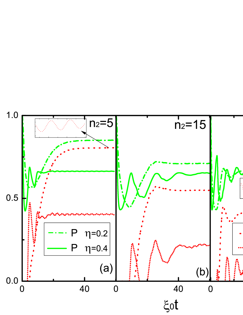
Figure 4: The temporal behavior of the logarithmic negativity $E_{N}$ (red lines) and the entanglement state purity $P$ (blue lines) for different values of the coupling $\eta$ and the site $n_{2}$ the second cavity located. The other parameters are the same as in Fig. 3.

In Fig. 3, the exact temporal evolution of the logarithmic negativity $E_{N}$ and the purity $P$ of the two-mode cavity field are plotted. From it, we see that the stationary logarithmic negativity $E_{N}^{s}=r\simeq 1.0$ and the purity $P_{s}\simeq 1$ for all the cases in which the first cavity siting at $n_{1}=1$ and the second cavity siting at $n_{2}=5,9,15$ with the coupling $\eta=\xi_{c}/\xi_{0}=0.08,0.05,0.01$, respectively. It also shows that with the increase of the distance between the two cavities, properly decreasing the cavity-waveguide coupling $\eta$ leads to the same steady and pure entangled state. This is because the oscillating profile of the spectral density $J_{ii}(\omega)$, as shown in Fig. 2, becomes narrower around the band center $\omega_{0}$ as the site $n_{2}$ increases. This in turn requires longer time for achieving the steady states as the coupling decreases. Thus, a proper choose of the cavity-waveguide coupling strength can yield the same entanglement degree and purity in the resonant case for the different distances between the two cavities, as shown in Fig. 3.

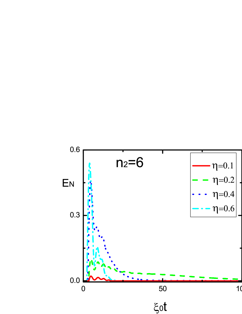
Figure 5: The temporal behavior of the logarithmic negativity $E_{N}$. The other parameters are the same as in Fig. 3.

In Fig. 4, the entanglement and purity are plotted for the enhanced cavity-waveguide couplings $\eta=0.2$ and $0.4$, with the different locations of the second cavity $n_{2}=5,15$ and $25$. It shows that as the cavity-waveguide coupling increases, the entanglement decreases by accompanying with some oscillations in the time evolution. The oscillation comes from the non-Markovian effect due to the back-action between the cavity and the waveguide when the cavity-waveguide coupling increases. Besides, one can also see that the entanglement sudden death and sudden birth occurs in the short-time regime with a relatively large cavity-waveguide coupling ($\eta=0.4$) and also a relatively long distance between the two cavities, see Fig. 4(b) and (c). In addition, as we see, the resulting entangled states become usually a mixed state as the cavity-waveguide coupling increases. By comparing Fig. 4 (a)-(c), one can also find that the entanglement decreases as the increase of the distance between the cavities as well as the cavity-waveguide coupling. Therefore, to maintain the high entanglement for the two distant cavities, a small cavity-waveguide coupling is more favorable in the resonant case.

Furthermore, as shown in Fig. 5 the entanglement appears in the case of the first cavity siting at $n_{1}=1$ and the second cavity siting at a even number of $n_{2}$. The exact numerical result shows that the entanglement between the two cavities can be generated under the relatively large coupling in a short time scale, but as the time goes the entanglement soon decays to zero. This is consistent with the analytical solution given by Eq. (17), where it is pointed out that the steady-state entanglement in this case can not exist if any one (or both) of the sites $n_{1}$ and $n_{2}$ of the two cavities is even.

III.2 $|\omega_{c}-\omega_{0}|\geq 2\xi_{0}$

To further investigate the controllability of the entanglement generation of the two spatially-separated nanocavities, we consider next the entanglement behavior for the cavity frequency $\omega_{c}$ outside the waveguide band, i.e., $|\omega_{c}-\omega_{0}|\geq 2\xi_{0}$. Let the first cavity site at $n_{1}=1$ and the second cavity locates at different sites. The temporal behaviors of the entanglement and the purity with different values of the cavity-waveguide coupling are plotted in Fig. 6. It shows that the entanglement exhibits a very regular oscillation with a even stronger entanglement degree $E_{N}^{\textrm{max}}>1$ for the input squeezing $r=1$. For example, the maximal entanglement $E_{N}^{\textrm{max}}\approx 1.94$ for the coupling $\eta=0.2$ in the present case, see Fig. 6(a). When the coupling is increased, the entanglement degree oscillates faster but the maximal entanglement is degraded a little bit only.

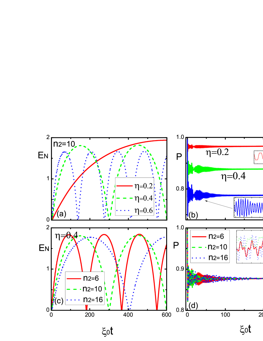
Figure 6: The temporal behavior of the logarithmic negativity $E_{N}$ and the purity $P$ for the different values of the coupling $\eta$ and the site $n_{2}$, while the cavity frequency $\omega_{c}=1.2\omega_{0}$ which stays the outside of the waveguide band. The other parameters are the same as in Fig. 3.

The above phenomenon can be understood as follows: in the weak coupling region, the damping rates $\gamma_{ij}=0$ since the spectral densities $J_{ij}(\omega_{c})=0$ when the frequency $\omega_{c}$ of the cavities lies outside the band of the waveguide. However, the cavity frequency shift, $\delta\bm{\omega}={\cal P}\int d\omega\frac{\bm{J}(\omega)}{\omega-\omega_{c}}$ does not vanish in this case. As a result, the reduced density matrix is purely determined by the effective Hamiltonian $H_{\textrm{eff}}=\sum_{i}(\omega_{c}+\delta\omega_{ii})a_{i}^{\dagger}a_{i}+\delta\omega_{12}(a_{1}^{\dagger}a_{2}+a_{2}^{\dagger}a_{1})$. In other words, an effective beam-splitter-type coupling (determined by the cross frequency shift $\delta\omega_{12}$) between the two cavities is induced by the waveguide, which results in the entanglement for the separated squeezing inputs. With the weak coupling solution of the propagating function $\bm{\mu}_{bm}(t)$ given in the Appendix, we have explicitly $\mu_{\textrm{bm},ii}=\cos(\delta\omega_{12}t)\textrm{e}^{-i\tilde{\omega}_{c}t}$ and $\mu_{\textrm{bm},12}=-i\sin{\delta\omega_{12}t}\textrm{e}^{-i\tilde{\omega}_{c}t}$, where $\tilde{\omega}_{c}=\omega_{c}+\delta\omega_{11}$ and $\delta\omega_{22}\approx\delta\omega_{11}$. The average values in Eq. (14) reduce to $\langle a_{i}^{\dagger}a_{i}\rangle=\sinh^{2}r$, $\langle a_{i}^{2}\rangle=\sinh r\cosh r\cos(2\delta\omega_{12}t)\textrm{e}^{-2i\tilde{\omega}_{c}t}$, $\langle a_{1}a_{2}\rangle=-i\sinh r\cosh r\sin(2\delta\omega_{12}t)\textrm{e}^{-2i\tilde{\omega}_{c}t}$, and $\langle a_{1}^{\dagger}a_{2}\rangle=0$. Thus, unlike the resonant case, the entanglement in this case is purely determined by the cross frequency shift $\delta\omega_{12}$. At the times when $\cos(2\delta\omega_{12}t)=0$, we have the nonzero average values $\langle a_{i}^{\dagger}a_{i}\rangle=\sinh^{2}r$ and $|\langle a_{1}a_{2}\rangle|=\sinh r\cosh r$, which corresponds to a pure two-mode squeezed vacuum state with the squeezing parameter $r$ gx . Accordingly, the entanglement degree at these times becomes optimal with the maximal logarithmic negativity

$$E_{N}^{\textrm{m}ax}=2r.$$ (19)

Fig. 6(a) shows that the maximal entanglement approaches the limit $2r$ when the coupling becomes sufficiently weak and the weak coupling solution given in Appendix is almost exact. With the cavity-waveguide coupling increase, the maximal entanglement is decreased a little bit, as shown in Fig. 6(a).

Fig. 6(b) depicts the corresponding purity of the entangled state. Since the damping rate vanishes in the weak coupling limit when the frequency of the cavities lies outside the waveguide band, the entangled state should be a pure state. Fig. 6(b) shows that for $\eta=0.2$, the exact numerical solution gives the purity $P\approx 0.97$ which is consistent with the weak coupling solution. When the cavity-waveguide coupling is increased, the purity of the waveguide-generated entanglement is decreased. Fig. 6(c) and (d) show further the dependence of the entanglement degree and the purity on the distance between the two nanocavities. Similar behavior of the oscillating entanglement is obtained as the cavity distance changes. This is due to the cross frequency shift $\delta\omega_{12}$ again, which is determined by the cross spectral density $J_{12}(\omega)$ that decreases slightly as $n_{2}$ increases for the fixed $n_{1}=1$. Besides, it is also found that the maximal entanglement and purity in the long-time region do not change obviously with the changes of the distance between the two nanocavities.

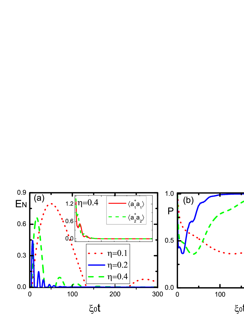
Figure 7: The temporal behavior of the logarithmic negativity $E_{N}$ and the purity $P$ for the cavity frequency within the waveguide band. Here we take $\omega_{c}=1.03\omega_{0}$ and the site $n_{2}=5$. The insert in the figure depicts the average photon numbers $\langle a_{i}^{\dagger}a_{i}\rangle$ of the two cavities. The other parameters are the same as in Fig. 3.

III.3 $|\omega_{c}-\omega_{0}|<2\xi_{0}$

Finally, we shall consider the case that the cavity frequency $\omega_{c}$ is not resonant with the band center but it still lies inside the waveguide band. In Fig.7 (a), the entanglement and the purity are plotted for the cavity sites $n_{1}=1$ and $n_{2}=5$ with the cavity frequency $\omega_{c}=1.03\omega_{0}$ at which the spectral density $J_{22}(\omega)=0$ for $\omega=\omega_{c}$ (see the red-dashed line in Fig. 2). In this case, the phenomenon of entanglement sudden death and sudden birth occurs in the weak coupling region. The existence of the entanglement sudden death and sudden birth originates from the fact that the damping $\gamma_{22}\approx 0$ and also $\gamma_{12}\approx 0$ for $\omega_{c}=1.03\omega_{0}$ so that the entanglement is purely governed by the cross frequency shift $\delta\omega_{12}$, which leads to the entanglement oscillation. In the long time limit, the entanglement is destroyed through the damping channel $\gamma_{11}\neq 0$. When the cavity-waveguide coupling increases, the entanglement only exists in a very short time and then quickly decay to zero significantly, which is quite different from the resonant case shown in Fig. 4. The insert in Fig. 7(a) is the intracavity average photon numbers $\langle a_{j}^{\dagger}a_{j}\rangle$ which approach to zero in the long-time limit. It tells that the cavity evolves asymptotically into a vacuum state. This is why the entanglement in the steady-state vanishes. The purity shown in Fig. 7(b) approaches to one in the steady-state limit because the steady state is just a trivial vacuum state.

In Fig. 8, we plot the entanglement for the cavity frequency $\omega_{c}=1.06\omega_{0}$, while the spectral density $J_{ii}(\omega)\neq 0~{}(i=1,2)$ at $\omega=\omega_{c}$. Then, both the decay channels $\gamma_{11}$ and $\gamma_{22}$ become active, and the entanglement is a combination effect of the the non-zero cross damping $\gamma_{12}$ and the non-zero cross frequency shift $\delta\omega_{12}$. Compared to that in Fig. 7(a), the entanglement here is enhanced significantly in the long-time regime. The phenomenon of the entanglement sudden death and sudden birth disappears in this case. As a result, we see that the entanglement generation can be easily controlled by changing the cavity frequency within the band of the waveguide.

Figure 8: The temporal behavior of the logarithmic negativity $E_{N}$ for the cavity frequency $\omega_{c}=1.06\omega_{0}$ and the second cavity locating at the site $n_{2}=5$. The other parameters are the same as in Fig. 3.

IV Conclusions

In conclusions, the generation of continuous variable entanglement between two spatially-separated nanocavities mediated by a CROW in photonic crystals is investigated. By solving the exact master equation for the cavity system coupled to the waveguide as a structured reservoir, the entanglement and the purity of the two-mode cavity field is analyzed in details for the initially-separated squeezing inputs. We found that the steady and pure entangled state of the two distant cavities can be generated for a weak cavity-waveguide coupling when the cavities is resonant with the band center of the waveguide. It also shows that the strong coupling of the cavities to the waveguide can lead to the phenomenon of entanglement sudden death and sudden birth. When the cavity frequencies lie outside the waveguide band, the optimal entanglement can be achieved by the cross frequency shift between the two cavities, which is induced by the waveguide. When the cavity frequencies are not resonant with the band center but still within the waveguide band, the entanglement can also exhibit the phenomenon of sudden death and sudden birth even for a weak cavity-waveguide coupling. By changing the cavity frequencies within the band of the waveguide, the entanglement and the occurrence of entanglement sudden death and birth can be easily controlled. These interesting results show that the waveguide, as a controllable structured reservoir, can be used to entangle efficiently the two spatially-separated nanocavities. More importantly, only a weak cavity-waveguide coupling is required for achieving the optimal entanglement. We expect that these interesting features can be realized in experiments and find its application in continuous variable quantum communication networks.

Appendix A A weak-coupling analytical solution

It should be pointed out that the master equation of Eq. (8) is exact, far beyond the Born-Markovian approximation and valid for arbitrary cavity-waveguide coupling. The back-action between the cavities and the waveguide is embedded into the time-dependent coefficients $\omega_{ij}(t)$ and $\bm{\gamma}(t)$ of Eq. (9), which are in turn determined completely by the propagating function $\bm{\mu}(t)$ of Eq. (10). Generally, it is not easy to obtain the analytical propagating function $\bm{\mu}(t)$. However, for a weak coupling, the analytical solution of the photon propagating function can be found as

$$\bm{\mu}_{bm}(t) =\textrm{e}^{-(\bm{\gamma}+i\bm{\bar{\omega}})t},$$ (20)

where the damping rate becomes time-independent: $\bm{\gamma}=\bm{J}(\omega_{c})/2$, and the waveguide-induced renormalized frequency is given by $\bm{\bar{\omega}}=\omega_{c}I+\bm{\delta\omega}$ with

$$\bm{\delta\omega}=\mathcal{P}\int\frac{d\omega}{2\pi}\frac{\bm{J}(\omega)}{\omega-\omega_{c}}.$$ (21)

Here $\mathcal{P}$ denotes the principle value of the integral. When the cavity frequency $\omega_{c}$ is resonant with the band center $\omega_{0}$ of the waveguide ($\omega_{c}=\omega_{0}$), the frequency shift $\bm{\delta\omega}=0$, and the explicit propagating function $\bm{\mu}_{bm}(t)$ in the weak-coupling limit is then given by

$$\mu_{\textrm{bm},11} =\frac{1}{\gamma_{11}+\gamma_{22}}[\gamma_{22}+\gamma_{11}\textrm{e}^{-(\gamma_{11}+\gamma_{22})t}]\textrm{e}^{-i\omega_{c}t},$$ (22a)

$$\mu_{\textrm{bm},22} =\frac{1}{\gamma_{11}+\gamma_{22}}[\gamma_{11}+\gamma_{22}\textrm{e}^{-(\gamma_{11}+\gamma_{22})t}]\textrm{e}^{-i\omega_{c}t},$$ (22b)

$$\mu_{\textrm{bm},12} =\mu_{\textrm{ bm},21}=-\frac{\gamma_{12}}{\gamma_{11}+\gamma_{22}}[1-\textrm{e}^{-(\gamma_{11}+\gamma_{22})t}]\textrm{e}^{-i\omega_{c}t},$$ (22c)

where the damping rates $\gamma_{ii}=(\frac{2\xi_{i}^{2}}{\xi_{0}})\sin^{2}(\frac{n_{i}\pi}{2})$ and the collective damping $\gamma_{12}=\sqrt{\gamma_{11}\gamma_{22}}$.

References

- (1) S. L. Braunstein and A. K. Pati, Quantum Information with Continuous Variables (Kluwer Academic, Dordrecht, 2003).
- (2) P. van Loock and S. L. Braunstein, Phys. Rev. Lett. 84, 3482 (2000).
- (3) X. Jia, X. Su, Q. Pan, J. Gao, C. Xie, and K. Peng, Phys. Rev. Lett. 93, 250503 (2004); J. Jing et al., Phys. Rev. Lett. 90, 167903 (2003); J. Zhang, G. Adesso, C. Xie, and K. Peng, Phys. Rev. Lett. 103, 070501(2009).
- (4) M. Y. Chen, M. W. Y. Tu and W. M. Zhang, Phys. Rev. B 80, 214538 (2009).
- (5) H. Shen, X. Su, X. Jia, and C. Xie, Phys. Rev. A 80, 042320. (2009).
- (6) N. C. Menicucci, S. T. Flammia, and O. Pfister, Phys. Rev. Lett. 101, 130501 (2008).
- (7) T. Aoki et al., Nat. Phys. 5, 541 (2009).
- (8) Y. Miwa et al., Phys. Rev. A 80, 050303 (R) (2009).
- (9) A. M. Marino, R. C. Pooser, V. Boyer, P. D. Lett, Nature 457, 859 (2009).
- (10) S. Pielawa, G. Morigi, D. Vitali, and L. Davidovich, Phys. Rev. Lett. 98, 240401 (2007).
- (11) G. X. Li, H. T. Tan, and M. Macovei, Phys. Rev. A 76, 053827 (2007); H. T. Tan, H. X. Xia, and G. X. Li, Phys. Rev. A 79, 063805 (2009).
- (12) Ch. Silberhorn et al., Phys. Rev. Lett. 86, 4267 (2001).
- (13) M. Notomi, Rep. Prog. Phys. 73, 096501 (2010).
- (14) L. M. Duan, M. D. Lukin, J. I. Cirac, and P. Zoller, Nature 414, 413 (2001).
- (15) H. J. Kimble, Nature 453, 1023 (2008).
- (16) A. Tudela, D. Cano, E. Moreno, L. Moreno, C. Tejedor, and F. Vidal, Phys. Rev. Lett. 106, 020501 (2011); Y. Yang, J. Xu, H. Chen, and S. Y. Zhu, Phys. Rev. A 82, 030304 (2010).
- (17) A. Wolf, G. D. Chiara, E. Kajari, E. Lutz, and G. Morigi, arXiv:1102.1838.
- (18) S. Noda, A. Chutinan, and M. Imada, Nature 407, 608 (2000);Y. Akahane, T. Asano, B. S. Song, and S. Noda, Nature, 425, 944 (2003).
- (19) A. Yariv, Y. Xu, R. K. Lee, and A. Scherer, Opt. Lett. 24, 711 (1999); M. Bayindir, B. Temelkuran, and E. Ozbay, Phys. Rev. Lett. 84, 2140 (2000).
- (20) M. Notomi, E. Kuramochi, and T. Tanabe, Nat. Photon. 2, 741 (2008).
- (21) T. Baba, Nat. Photon. 2, 465 (2008).
- (22) Y. Liu, Z. Wang, M. Han, S. Fan, and R. Dutton, Opt. Express 13, 4539 (2005).
- (23) A. Politi, M. J. Cryan, J. G. Rarity, S. Yu and J. L. O’Brien, Science 320 646 (2008); J. L. O’Brien1, A. Furusawa, and J. Vuckovic, Nat. Photon. 3, 687 (2009).
- (24) L. Sansoni et al., Phys. Rev. Lett. 105, 200503 (2010).
- (25) J. S. Prauzner-Bechcicki, J. Phys. A 37, 173 (2004).
- (26) J. H. An, and W. M. Zhang, Phys. Rev. A 76, 042127 (2007); J. H. An, M. Feng, and W. M. Zhang, Quantum Inf. Comput. 9, 0317 (2009).
- (27) J. P. Paz and A. J. Roncaglia, Phys. Rev. Lett. 100, 220401 (20080); Phy. Rev. A 79 032102 (2009).
- (28) S. Maniscalco, S. Olivares, and M. G. A. Paris, Phys. Rev. A 75, 062119 (2007).
- (29) G. X. Li, L. Sun, and Z. Ficek, J. Phys. B 43, 135501 (2010).
- (30) H. N. Xiong, W. M. Zhang, X. G. Wang, and M. H. Wu, Phys. Rev. A 82, 012105 (2010).
- (31) M. H. Wu, C. U. Lei, W. M. Zhang, and H. N. Xiong, Opt. Express 18, 18407 (2010).
- (32) H. T. Tan and W. M. Zhang, Phys. Rev. A 83, 032102 (2011).
- (33) C. U. Lei and W. M. Zhang, arXiv:1011.4570.
- (34) T. Yu, J. H. Eberly, Phys. Rev. Lett. 93, 140404 (2004).
- (35) M. Notomi, Rep. Prog. Phys. 73, 096501 (2010).
- (36) G. Vidal and R. F. Werner, Phys. Rev. A 65, 032314 (2002).
- (37) R. P. Feynman and F. L. Vernon, Ann. Phys. (NY) 24, 118 (1963).
- (38) W. M. Zhang, D. H. Feng, and R. Gilmore, Rev. Mod. Phys. 62, 867 (1990).
- (39) S. H. Xiang, B. Shao, and K. H. Song, Phys. Rev. A 78, 052313 (2008).
- (40) C. Hörhammer and H. Büttner, Phys. Rev. A 77, 042305 (2008).
- (41) M. O. Scully and M. S. Zubairy, Quantum Optics (Cambridge University Press, Cambridge, UK, 1997).
- (42) G. X. Li, H. T. Tan, and S. S. Ke, Phys. Rev. A 74, 012304 (2006).