Abstract

Historical linguistics aims at inferring the most likely language phylogenetic tree starting from information concerning the evolutionary relatedness of languages. The available information are typically lists of homologous (lexical, phonological, syntactic) features or characters for many different languages: a set of parallel corpora whose compilation represents a paramount achievement in linguistics.

From this perspective the reconstruction of language trees is an example of inverse problems: starting from present, incomplete and often noisy, information, one aims at inferring the most likely past evolutionary history. A fundamental issue in inverse problems is the evaluation of the inference made. A standard way of dealing with this question is to generate data with artificial models in order to have full access to the evolutionary process one is going to infer. This procedure presents an intrinsic limitation: when dealing with real data sets, one typically does not know which model of evolution is the most suitable for them. A possible way out is to compare algorithmic inference with expert classifications. This is the point of view we take here by conducting a thorough survey of the accuracy of reconstruction methods as compared with the Ethnologue expert classifications. We focus in particular on state-of-the-art distance-based methods for phylogeny reconstruction using worldwide linguistic databases.

In order to assess the accuracy of the inferred trees we introduce and characterize two generalizations of standard definitions of distances between trees. Based on these scores we quantify the relative performances of the distance-based algorithms considered. Further we quantify how the completeness and the coverage of the available databases affect the accuracy of the reconstruction. Finally we draw some conclusions about where the accuracy of the reconstructions in historical linguistics stands and about the leading directions to improve it.

Introduction

The last few years have seen a wave of computational approaches devoted to historical linguistics [1, 2, 3], mainly centred around phylogenetic methods. While the first aim of phylogeny reconstruction is that of classifying a set of species (viruses, biological species, languages, texts), the information embodied in the inferred trees goes beyond a simple classification knowledge. Statistical tools [4, 5, 6, 7, 8, 9], for instance, permit to assign time weights to the edges of a phylogenetic tree, giving the opportunity to gather information about the past history of the whole evolutionary process. These techniques have been successfully employed to investigate features of human prehistory [10, 11, 12, 13, 14, 15].

The application of computational tools in historical linguistics is not a novel one, since it dates back to the 50’s, when Swadesh [16, 17] first proposed an approach to comparative linguistics that involved the quantitative comparison of lexical cognates, an approach named lexicostatistics. The most important element here is the compilation, for each language being considered, of lists of universally used meanings (hand, mouth, sky, I, ..). The initial set of meanings included $200$ items which were then reduced down to $100$, including some new terms which were not in his original list. Each language is represented by its specific list and different languages can be compared exploiting the similarity of their lists. The similarity is assessed by estimating the level of cognacy between pairs of words. The higher the proportion of cognacy the closer the languages are related. Though originally cognacy decisions was solely based on the work of trained and experienced linguists, automated methods have been progressively introduced (see [18] and for a recent overview  [19]) that exploit the notion of Edit Distance (or Levenshtein Distance) [20] between words, considered as strings of characters. The computation of the Edit Distance between all the pairs of homologous words in pairs of languages leads to the computation of a “distance” between pairs of languages. This value is entered into a $N\times N$ table of distances, where $N$ is the number of languages being compared. This distance matrix can then be submitted to distance-based algorithms for the purpose of generating trees showing relationships among languages.

The construction of the distance matrix is of course a crucial step since the reliability of the reconstruction of the evolutionary history, i.e., the outcome of a phylogenetic reconstruction method, strongly depends on the properties of the distance matrix. In particular if the matrix features the property of being additive, there are algorithms that guarantee the reconstruction of the unique true tree (see [21] for a recent overview). A distance matrix is said to be additive if it can be constructed as the sum of a tree’s branch lengths. When considering experimental data, additivity is almost always violated. Violations of additivity can arise both from experimental noise and from properties of the evolutionary process underlying the data. One of the possible sources of violation of additivity is the so-called back-mutation: in old phylogenies a single character can experience multiple mutations. In this case the distances between taxa are no longer proportional to their evolutionary distances. In historical linguistics this would happen if one was considering meanings that change very rapidly. For this reason linguists are typically interested in removing from the lists all the fast-evolving meanings. Of course this is not an easy task, bringing inextricably with itself a fair amount of arbitrariness in the choice. Along the same lines another crucial difficulty in lexicostatistics concerns the rate of change of the individual meanings. Different meanings, represented in each language by different words, evolve with different rates of change. In a biological parallel one would say that the mutation rate, i.e., the rate over which specific words undergo morphological, phonetic or semantic changes, are meaning dependent. This effect again is not easily cured and again different choices of the list composition could lead to different reconstructions. Finally another source of deviations from additivity is the so-called horizontal-transfer. The reconstruction of a phylogeny from data underlies the assumption that information flows vertically from ancestors to offspring. However, in many processes information also flows horizontally. In historical linguistics borrowings represent a well-known confounding factor for a correct phylogenetic inference.

All the fore-mentioned difficulties in the reconstruction of phylogenetic trees strongly call for reliable methods to evaluate the reconstructed phylogenies. Along with this it comes the need of valid benchmarks for determining the reliability of the different methods used to reconstruct phylogenetic trees. The standard way of testing the proposed algorithms is the construction of models to generate artificial phylogenies [21, 22, 23], so that the algorithmic results can be directly compared with the true, known, observables of interest. However, in doing that, one makes inevitable assumptions on the evolutionary processes of interest, which can in turn influence the reconstruction performance. To overcome this problem, we consider here an application of phylogenetic tools to historical linguistics. This field offers a good reference point, since classifications made with phylogenetic tools can be compared with catalogues of languages made by experts. We focus in particular on the Ethnologue classification. The Ethnologue can be described as a comprehensive catalogue of the known languages spoken in the world [24], organized by continent and country, being thus a valid reference point to evaluate trees inferred using phylogenetic algorithms (see section Data for details).

Here we evaluate trees reconstructed using distance-based phylogenetic methods against the Ethnologue trees. To this end it is important to set the tools to compare expert Ethnologue trees and phylogenetically inferred trees. There are several standard ways of measuring the distance between two phylogenetic trees. Here we take into account two of them, the Robinson-Foulds (RF) distance [25], which counts the number of bipartitions on which the two trees differ, and the Quartet Distance (QD) [26], which counts the number of subset of four taxa on which the two trees differ.

A technical problem when comparing Ethnologue classifications and inferred trees is that typically Ethnologue trees are not binary while all the inferred trees are. In order to overcome this difficulty we introduce two incompatibilities scores, which are two generalizations of both the Robinson-Foulds [25] and the Quartet Distance measures [26]. We present results obtained on a wide range of language families. This allows to compare different definitions of distances as well as different reconstruction algorithms.

The outline of the paper is as follows. We first introduce the Ethnologue [24] project and both the Automated Similarity Judgement Program (ASJP)[27] and the Austronesian Basic Vocabulary Database (ABVD) [28] database we used in our analysis, pointing out some structural and statistical features that will be relevant in our discussion. Next we introduce some mathematical tools. We define both the Levenshtein Normalized Distance (LDN) and the Levenshtein Divided Normalized Distance(LDND) [19] to compute a “distance” between lists of word. The quantification of the accuracy of the inference of language trees we present is achieved with the Robinson-Foulds distance (RF) [25] and the Quartet Distance (QD) [26]. These are two standard definitions of distances between trees. We introduce and characterize such mathematical tools and we also present generalizations of these two scores, in order to adapt them for the comparison of binary (inferred) and non-binary (classifications) trees. We then present the results of the comparisons between the Ethnologue classifications and the language trees inferred based on the ASJP database. We first consider the ASJP database in order to perform a worldwide, i.e., large-scale, analysis. Finally we point out how some of the properties of word-lists, such as the completeness and the coverage, affect the accuracy of the reconstruction. To this end we present a comparative analysis on the inference of the Austronesian family, making use of both the ASJP and the ABVD database. The Supporting Information provides an extensive account of the whole set of results we obtained.

Materials and Methods

Data

The Ethnologue can be described as a comprehensive catalogue of the known languages spoken in the world [24]. The Ethnologue was founded by R.S. Pittman in 1951 as a way to communicate with colleagues about language development projects. Its first edition was a ten-page informal list of $46$ language and language group names. As of its sixteenth edition, Ethnologue has grown into a comprehensive database that is constantly being updated as new information arrives. As of now it contains close to $7000$ language descriptions, organized by continent and country, which can be represented as a tree. As already mentioned, this tree is not always fully specified since it contains a lot of non-binary structures, in which the details of the phylogeny are not given due to a lack of certain information. Figure 1 illustrates geographically how the Ethnologue classifications deviate from being purely binary.

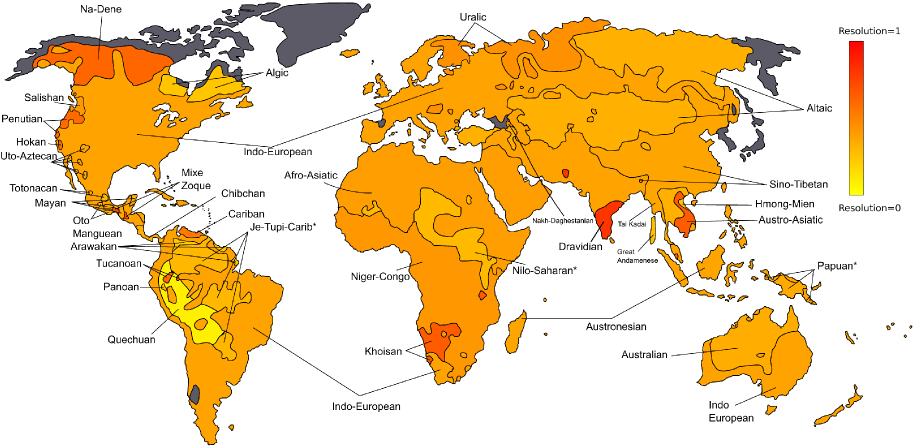
Figure 1: Ethnologue resolution power. This map represents the Ethnologue resolution power in the different world locations. Red areas corresponds to regions where the Ethnologue classification is completely binary, i.e., correspond to a tree in which each internal node has exactly two child nodes. Yellow areas corresponds to fully unspecified trees, featuring only a star structure. Grey areas are those for which no data are present in the databases we consider to reconstruct language trees. Asterisks are for regions which include more than one language family (we report in the Supporting Information the list of such families).

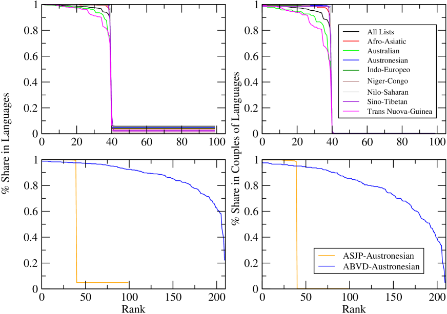
Figure 2: Top: Statistics of the ASJP database. (left panel) Fraction-rank plot: for each word in the lists of words of the Automated Similarity Judgement Project (ASJP), we measured the fraction of languages containing it. The plot reports this fraction vs. its rank. In the $100$-items lists in the ASJP database, only $40$ meanings are shared by almost $100\%$ of the languages for each family. (right panel) Ranked fraction of pairs of languages sharing each specific word vs. rank. Again only $40$ meanings are shared by almost $100\%$ of the pairs of languages. Bottom: Statistical measures on the ABVD database. (left panel) Fraction-rank plot: for each word in the lists of words of the Austronesian Basic Vocabulary Database (ABVD), we measured the fraction of languages containing it. The plot reports this fraction vs. its rank. (right panel) Ranked fraction of pairs of languages sharing each specific word vs. rank. For sake of a rough comparison we also reported the same quantities measured on the Austronesian family of the ASJP database. The ASJP includes $40$ words up to a maximum of almost $100\%$ of the languages, whereas in the ABVD the percentage of coverage is at least of $50\%$ for almost all the words in the list. Limited to the $40$ most shared words the ASJP database features a slightly larger coverage than the ABVD database.

The Automated Similarity Judgement Program (ASJP)[27] includes $100$-items word lists of about 50 families of languages throughout the world. These lists are written in a standardized orthography (ASJP code) which employs only symbols of the standard QWERTY keyboard, defining vowels, consonants and phonological features. The full database is available at http://email.eva.mpg.de/~wichmann/ASJPHomePage.htm. Figure 2 (top) reports two statistical measures on the database to quantify its completeness. In particular we report the ranked fraction of languages containing a word for a specific meaning vs. the rank (left panel) and the ranked fraction of pairs of languages sharing a word (not necessarily a cognate) for a specific meaning vs. the rank (right panel). The second measure helps in understanding how accurate, from a statistical point of view, the computation of the distance between two languages averaging the Levenshtein distances of all the words for homologous meanings. Evidently the database is very complete up to $40$ meanings.

The Austronesian Basic Vocabulary Database (ABVD) [28] contains lexical items from $737$ languages (as of January 2011) spoken throughout the Pacific region. Most of these languages belong to the Austronesian language family, which is the largest family in the world. Due to the extended and phonetic characters used for the lexical orthography, all the information is encoded in the Unicode format UTF-8. The web site of the database is http://language.psy.auckland.ac.nz/austronesian/ and we downloaded it on October, the 4th 2010. We focused in particular on a subset of $305$ languages that are present both in the ASJP database and in the Ethnologue classification. Figure 2 (bottom) reports the same quantities of Figure 2 (top) for the ABVD database. It is evident how, limited to the Austronesian family, the ABVD database features an overall larger (with respect to the ASJP database) number of meanings across all the languages considered. The level of coverage decreases progressively as one increases the number of meanings. A word of caution is in order. It is of course not possible to compare the completeness of the ASJP and the ABVD databases since they refer to two completely different projects with different aims: ASJP aiming at a full coverage of the Swadesh lists on all the world languages and ABVD being focused only on the Austronesian languages. It is nevertheless interesting to compare them only as for the Austronesian family is concerned. We shall come back on this point when we shall compare the accuracy of the reconstructed trees using different databases.

Distance between languages

In our studies we represent a language by its list of words for the different meanings. The distance between two languages is based on the distance between pairs of words corresponding to homologous meanings in the two lists. The distance between two words is computed by means of the Levenshtein distance (LD). The LD is a metric to quantify the difference between two sequences and it is defined as the minimum number of edit operations needed to transform one string into the other, the allowable edit operations being insertion of a character, deletion of a character and substitution of a single character.

Once the distance between pairs of words is specified, two different definitions of distances between languages have been introduced [29, 30, 31, 19]: the Levenshtein Distance Normalized (LDN) and a revised interpretation of it named Levenshtein Distance Normalized Divided (LDND). Both these definitions have been introduced to correctly define distances between languages, instead of simply considering an average of the LD distance between words corresponding to homologous meanings in the lists.

According to LDN definition [29, 30], given two words $\alpha_{i}$ and $\beta_{j}$, their distance is given by:

$$LDN(\alpha_{i},\beta_{j})=\frac{LD(\alpha_{i},\beta_{j})}{l(\alpha_{i},\beta_{j})}$$ (1)

where $LD(\alpha_{i},\beta_{j})$ is the LD between the two words and $l(\alpha_{i},\beta_{j})$ is the number of characters of the longest of the two words $\alpha_{i}$ and $\beta_{j}$ . This normalization has been introduced in order to avoid biases due to long words, giving in this way the same weight to all the words in the lists. Starting from this definition, let us now assume that the number of languages is $N$ and the list of meanings for each language contains $M$ items. Each language in the group is labelled by a Greek letter (say $\alpha$) and each word of that language by $\alpha_{i}$, with $1\leq i\leq M$. Then, two words $\alpha_{i}$ and $\beta_{j}$ in the languages $\alpha$ and $\beta$ have the same meaning (they correspond to the same meaning) if $i=j$ . The LDN between the two languages is thus:

$$LDN(\alpha,\beta)=\frac{1}{M}\underset{i}{\sum}LDN(\alpha_{i},\beta_{i})$$ (2)

Another definition of distance between pair of languages has been introduced in [31] in order to avoid biases due to accidental orthographical similarities in two languages:

$$\Gamma(\alpha,\beta)=\frac{1}{M(M-1)}\underset{i\neq j}{\sum}LDN(\alpha_{i},\beta_{i})$$ (3)

The LDND distance between two languages is then defined as:

$$LDND(\alpha,\beta)=\frac{LDN(\alpha,\beta)}{\Gamma(\alpha,\beta)}$$ (4)

A comparison of the two definition of distances has been presented in [19]. In the following we consider both these definitions of distances between languages; the dissimilarity-matrices computed according to them will be the starting point for the inference of the family trees, which will be compared with the corresponding Ethnologue classifications.

Robinson-Foulds, Quartet Distance and generalizations

All the conclusions drawn in this work will be based on a quantitative comparison between inferred trees and the Ethnologue classifications. To this end it is important to recall how to measure the distance between two tree topologies. Here we recall in particular the mathematical definitions of two metrics between trees: the Robinson-Foulds distance (RF) [25] and the Quartet Distance (QD) [26].

The Robinson-Foulds (RF) distance between two trees counts the number of bipartitions on which the two trees differ. If we delete an internal edge in a tree, the leaves will be divided in two subsets; we call this division a bipartition. Here we consider a normalized version of the RF distance, which counts the percentage of unshared bipartitions between two trees. More formally, let ${\cal{T}}1$ and ${\cal{T}}2$ be two trees with the same set of leaves, then:

$$RF({\cal{T}}1,{\cal{T}}2)=\frac{i({\cal{T}}1)+i({\cal{T}}2)-2e({\cal{T}}1,{\cal{T}}2)}{i({\cal{T}}1)+i({\cal{T}}2)}$$ (5)

where $i({\cal{T}})$ denotes the set of internal edge of ${\cal{T}}$ and $e({\cal{T}}1,{\cal{T}}2)$ denotes the number of pairs of identical bipartitions in ${\cal{T}}1$ and ${\cal{T}}2$. The RF distance is a metric in the space of trees, whose value ranges from $0$ (if and only if ${\cal{T}}1={\cal{T}}2$ ) to $1$.

Another possible distance between two trees is the Quartet Distance (QD). In a tree of $N$ leaves, we can look at the subtrees defined by sets of four taxa (quartets). In the general case of non fully resolved trees, a butterfly names a quartet in which the two pairs of leaves are divided by an internal edge and a star a quartet in which the leaves are all linked to the same node. The QD between two trees counts the number of non compatible quartets in the two trees. It is defined as:

$$QD({\cal{T}}1,{\cal{T}}2)=\frac{q({\cal{T}}1)+q({\cal{T}}2)-2s({\cal{T}}1,{\cal{T}}2)-d({\cal{T}}1,{\cal{T}}2)}{\mathrm{norm}(N)}$$ (6)

where $q({\cal{T}})$ is the total number of butterflies in ${\cal{T}}$, $s({\cal{T}}1,{\cal{T}}2)$ is the number of identical butterflies in ${\cal{T}}1$ and ${\cal{T}}2$ and $d({\cal{T}}1,{\cal{T}}2)$ is the number of different butterflies in the two trees. The normalization factor is the number, $\mathrm{norm}(N)=\binom{N}{4}$, of quartets in a tree of $N$ taxa. The QD, as well as the RF distance, is a metric in the space of trees, whose value ranges from $0$ (if and only if ${\cal{T}}1={\cal{T}}2$ ) to $1$.

In [32, 33] a deep analysis of both RF and QD is reported, pointing out the different information the two measures convey. In limiting cases, pairs of trees that have the same RF distance but very different QD, and vice-versa, are also shown. In Fig. 3, quoting an enlightening example in [32, 33], we show how the RF and the QD measures weigh a swapping event of two subtrees in a tree. In this case the RF distance is equal to the number of edges in the path between the swapped subtrees, while the QD is sensitive to the size of the subtrees. The RF is then a good measure if we are interested in measuring how far apart subtrees are moved in one tree with respect to another. When we are interested instead in the size of the displaced subtrees, the quartet distance is a more adequate measure.

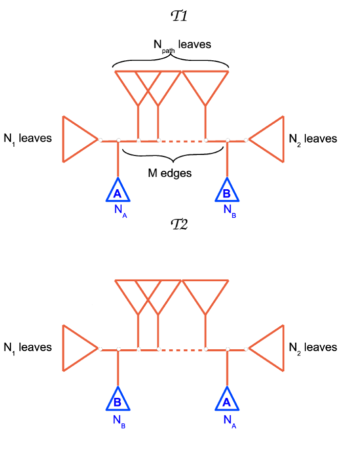
Figure 3: Robinson-Foulds and Quartet Distance: errors due to a displacement of a couple of subtrees. The trees ${\cal{T}}_{1}$ and ${\cal{T}}_{2}$ are different because of the swap of the subtrees A and B. While computing the distance between ${\cal{T}}_{1}$ and ${\cal{T}}_{2}$, the Robinson-Foulds distance detects all the $M$ edges in the path as errors, regardless of the size of the subtrees attached to them. The number of wrong butterflies quartets counted as errors with the Quartet Distance is expressed by $N_{1}N_{A}(N_{path}N_{B}+N_{path}N_{2}+N_{B}N_{2})+N_{2}N_{B}(N_{1}N_{path}+N_{path})N_{A}$: the QD thus depends on the size of the subtrees.

The Ethnologue classification provides a coarse grained grouping of subsets of languages, often leading to trees that are not fully resolved, i.e., that are not binary. For that reason, it is important to correct the biases suffered by the RF and QD distances while comparing binary with non binary trees.

Figure 4 illustrates a situation when a binary tree (${{\cal{T}}_{i}}$) is compared with a non-binary one (${\cal{T}}_{e}$). Both the RF and the QD give a non zero distance between the two trees: some partitions of ${{\cal{T}}_{i}}$ are in fact not present in ${{\cal{T}}_{e}}$. It is important to consider, however, that in the case we are considering (algorithmic inference versus Ethnologue classification) non-binary classification is simply due to a lack of information or details that would lead to a finer classification. We would like to be able to distinguish intrinsic contradictions between reconstructed binary trees and the Ethnologue classifications from errors due to the low level of resolution of the Ethnologue trees. It is with this aim in mind that we introduce a generalization of both the RF distance and the QD.

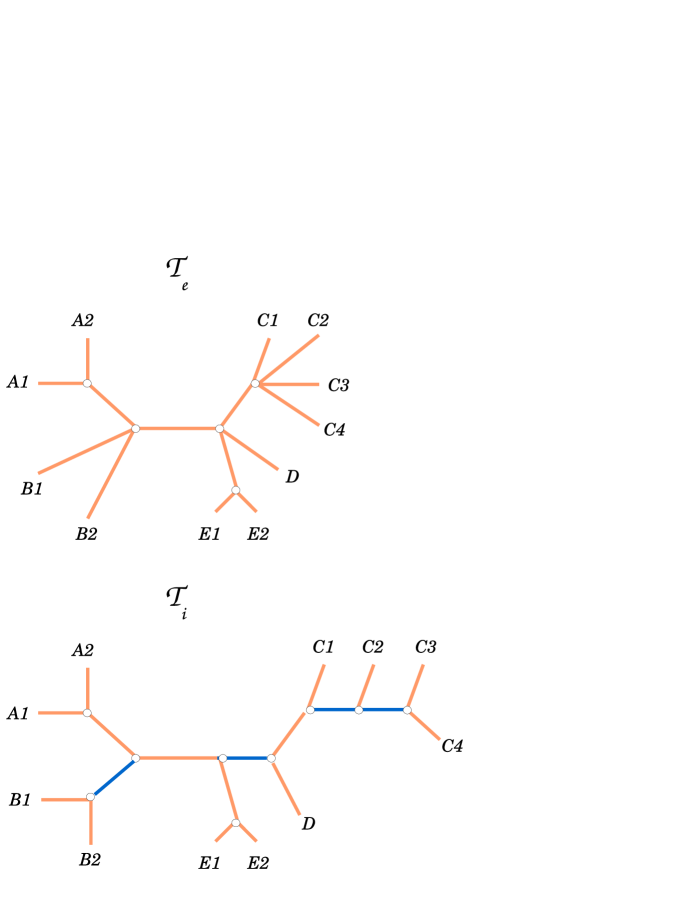
Figure 4: Non-binary nodes: biases of errors. The standard Robinson-Foulds distance and the Quartet Distance have a bias when comparing binary trees with non-binary classifications. The difference between tree ${\cal{T}}_{e}$ and ${{\cal{T}}_{i}}$ is that ${\cal{T}}_{i}$ shows a more fine grained classification. The two trees, however, are not conflicting, since ${\cal{T}}_{i}$ is simply a refinement of the classification ${\cal{T}}_{e}$. The RF distance will count every internal edge (blue ones in ${{\cal{T}}_{i}}$) of this refinement as errors, since they are not in ${\cal{T}}_{e}$. The QD will count every quartet including the blue edges as errors, since all these quartets are stars in ${\cal{T}}_{e}$. The generalized measures we introduce correctly give a null score between ${\cal{T}}_{e}$ and ${{\cal{T}}_{i}}$ in the example.

Let ${\cal{T}}_{e}$ be the Ethnologue (non necessarily binary) tree and ${\cal{T}}_{i}$ the inferred tree, then we define the Generalized Robinson-Foulds (GRF) score as:

$$GRF({\cal{T}}_{i},{\cal{T}}_{e})=\frac{i({\cal{T}}_{i})-e_{\mathrm{mod}}({\cal{T}}_{i},{\cal{T}}_{e})}{i({\cal{T}}_{i})}$$ (7)

where $i({\cal{T}}_{i})$ denotes the number of internal edge of ${\cal{T}}_{i}$ and $e_{\mathrm{mod}}({\cal{T}}_{i},{\cal{T}}_{e})$ the number of bipartitions in ${\cal{T}}_{i}$ compatible with those in ${\cal{T}}_{e}$. Intuitively, a bipartition in ${\cal{T}}_{i}$ is said to be compatible with a bipartition in ${\cal{T}}_{e}$ if it does not contradict any of the bipartitions induced by cutting an edge in ${\cal{T}}_{e}$. More rigorously, the compatibility of a bipartition $b$ of ${\cal{T}}_{i}$ with the tree ${\cal{T}}_{e}$ is defined as follows. Let us call $b_{1}$ and $b_{2}$ the two sets defining $b$, and $a_{1}^{i},a_{2}^{i}$ the two sets defining the $i$-th bipartition of ${\cal{T}}_{e}$. The partition $b$ is compatible with the tree ${\cal{T}}_{e}$ if for each bipartition $i$ of ${\cal{T}}_{e}$, the following is true: $b_{1}\subseteq a_{1}^{i}$, or $b_{1}\subseteq a_{2}^{i}$, or $b_{2}\subseteq a_{1}^{i}$, or $b_{2}\subseteq a_{2}^{i}$.

Let us note that the GRF is not symmetric in the two trees: this guarantees that a refinement edge is not counted as an error and the incomplete resolution of ${\cal{T}}_{e}$ does not affect the measure of the reliability of the reconstructed tree. We can verify that the GRF distance between ${\cal{T}}_{i}$ and ${\cal{T}}_{e}$ in figure 4is zero.

The QD is more straightforwardly generalized. We define the Generalized Quartet Distance (GQD) score as:

$$GQD({\cal{T}}_{i},{\cal{T}}_{e})=\frac{d({\cal{T}}_{i},{\cal{T}}_{e})}{\mathrm{norm}({\cal{T}}_{e})}$$ (8)

where $d({\cal{T}}i,{\cal{T}}e)$, as already introduced, denotes the number of different butterflies in ${\cal{T}}_{i}$ and ${\cal{T}}_{e}$. Again, this definition guarantees that all the star quartets in the Ethnologue trees will not be counted as errors. The normalization factor is equal to the number of butterfly quartets in ${\cal{T}}_{e}$: $\mathrm{norm}({\cal{T}}_{e})=q({\cal{T}}_{e})$, recalling the definition of $q({\cal{T}})$ given in eq. 6.

Let us stress again that both these generalized scores are neither symmetric or metric, since we are simply interested in quantifying the degree of accuracy of a binary tree with respect to an already known classification. With this definition, both the GQD and the GRF score give null scores if a classification tree is compared with one of its possible refinements, while one would get a score of $1$ for inferred trees in total disagreement with the classification. In the Supplementary Information we report a measure of the correlation of the accuracy of the trees reconstruction with the Ethnologue resolution, as measured both with the standard measures and with the generalized ones, showing how the last ones correctly remove the biases due to the incomplete Ethnologue classification.

Results

Inferred trees vs. Ethnologue

In this section we present the results of the comparison between the Ethnologue classification and the language trees inferred by state-of-the-art distance based algorithms. We first consider the ASJP database in order to perform a worldwide, i.e., large-scale, analysis.

Starting from the word lists of the ASJP project, we first estimated the distance matrices among all the languages in each family. We used both the LDN (2) and the LDND (4) distances, so we had two classes of distance matrices as an input for distance-based algorithms. We use three distance-based algorithms: Neighbour-Joining (NJ) [34], FastME [35] (belonging to the class of Balanced Minimum Evolution (BME) algorithms) and FastSBiX [22, 23], a recently introduced Stochastic Local Search algorithm. Each distance matrix was submitted as input to the three algorithms, which gives, for each language family, a total of six possible inferred trees.

To quantify the accuracy of the inferred trees, for each language family we computed the Generalized Robinson-Foulds score (GRF) and the Generalized Quartet Distance (GQD) of the inferred trees with the corresponding Ethnologue classifications. Tables 1 and 2 illustrate in an aggregate way the results obtained using the ASJP database. In particular we report, for each continent, the mean and the variance, across all the language families in that continent, of the values of the GRF and of the GQD between the inferred trees and the corresponding Ethnologue classifications, using both the LDN and the LDND distances. For each continent we considered all the language families present in the ASJP database.

As already mentioned, the GRF and the GQD are two complementary measures of the disagreement between the inferred tree and the expert classification. The GRF quantifies the percentage of wrong edges in the inferred trees, while the GQD counts how many quartets in the Ethnologue tree are different butterflies than in the reconstructed tree. In both cases the performance of the different algorithms always look very similar, though in almost all cases the noise reduction made by FastSBiX corresponds to a slightly better ability in reconstructing the correct phylogenies. FastSBiX features indeed the lowest average scores and, in many cases, the lowest variances. As for the distance matrix, our results show how better performances are obtained, on average, by using the LDND distance (4). The last column of the tables, named “RANDOM”, shows the error one would have for a randomly reconstructed tree. This information is useful to correctly appreciate the algorithmic ability of inferring the correct phylogenetic relationships. While in fact we correct the distance measures in order to avoid biases due to non binary classification, it is evident that it is easier to be consistent with a very coarse grained classification than with a finer one. In order to take into account this observation, we can compare the errors made by the reconstruction algorithms with the errors a completely randomly constructed tree (with the same leaves) would feature. The RANDOM columns of tables 1 and 2 report averages over 10 realizations of the GRF and the GQD between a randomly reconstructed tree and the Ethnologue classification.

Figures 5 and 6 report the histograms of the accuracies obtained using the FastSBiX algorithm for each continent and worldwide: large fluctuations exist both within each continent and worldwide (The complete set of results for each language family and for all the accuracy scores is presented as Supporting Information in the tables 6, 7, 8 and 9).

We finally give a pictorial view of the accuracy of the reconstruction algorithm across the planet. Figure 7 illustrates the Generalized Quartet Distance for the different language families on the world map, normalized with the corresponding random value. More specifically, the color codes, for each family $f$, the following quantity:

$$X_{f}=2\frac{GQD(f)}{GQD_{random}(f)}$$ (9)

where $GQD_{random}(f)$ represents the mean value of the GQD obtained averaging over $10$ randomly reconstructed trees with the same leaves (languages) of the family $f$. $X_{f}$ quantifies the level of accuracy of the reconstruction with respect to a null model. The multiplicative factor $2$ is included for the sake of better visualization: $X_{f}=1$ indicates a $GQD(f)$ equal or higher to half of the random tree distance $GQD_{random}(f)$.

GENERALIZED ROBINSON-FOULDS SCORE
	LDN			LDND
	Neighbour-Joining	FastME	FastSBiX	Neighbour-Joining	FastME	FastSBiX	RANDOM
AFRICA
Mean	0.2872	0.2845	0.2749	0.2859	0.2743	0.2729	0.7888
Variance	0.0327	0.0322	0.0329	0.0324	0.0323	0.0332	0.1945
EURASIA
Mean	0.3152	0.3116	0.2999	0.3056	0.2930	0.2998	0.9063
Variance	0.0244	0.0238	0.0138	0.0200	0.0200	0.0108	0.0313
PACIFIC
Mean	0.1228	0.1271	0.1092	0.1200	0.1178	0.1083	0.7282
Variance	0.0173	0.0182	0.0181	0.0174	0.0177	0.0177	0.1422
AMERICA
Mean	0.3084	0.2885	0.2797	0.2972	0.3080	0.3023	0.8949
Variance	0.0673	0.0600	0.0522	0.0673	0.0726	0.0654	0.0525

Table 1: Accuracy of the reconstructions as measured with the Generalized Robinson-Foulds (GRF). For each continent we report the average and the variance of the GRF over all the languages spread on the continent. The different columns correspond to the two different ways of constructing the distance matrix (LDN and LDND) and to the three distance-based algorithms considered. The last column labelled RANDOM reports the results for the null model considered. See the main text for details.

GENERALIZED QUARTET DISTANCE
	LDN			LDND
	Neighbour-Joining	FastME	FastSBiX	Neighbour-Joining	FastME	FastSBiX	RANDOM
AFRICA
Mean	0.1379	0.1872	0.1379	0.1094	0.1048	0.0855	0.4781
Variance	0.0072	0.0164	0.0069	0.0047	0.0045	0.0044	0.0601
EURASIA
Mean	0.1911	0.1787	0.1721	0.1716	0.1676	0.1661	0.6437
Variance	0.0378	0.0387	0.0399	0.0386	0.0385	0.0355	0.0011
PACIFIC
Mean	0.0864	0.0901	0.0662	0.0829	0.0858	0.0706	0.4893
Variance	0.0096	0.0091	0.0085	0.0079	0.0109	0.0070	0.0691
AMERICA
Mean	0.1595	0.1536	0.1569	0.1618	0.1646	0.1600	0.6057
Variance	0.0252	0.0245	0.0235	0.0244	0.0281	0.0269	0.0339

Table 2: Accuracy of the reconstructions as measured with the Generalized Quartet Distance (GQD). For each continent we report the average and the variance of the GQD over all the languages spread on the continent. The different columns correspond to the two different ways of constructing the distance matrix (LDN and LDND) and to the three distance-based algorithms considered. The last column labelled RANDOM reports the results for the null model considered. See the main text for details.

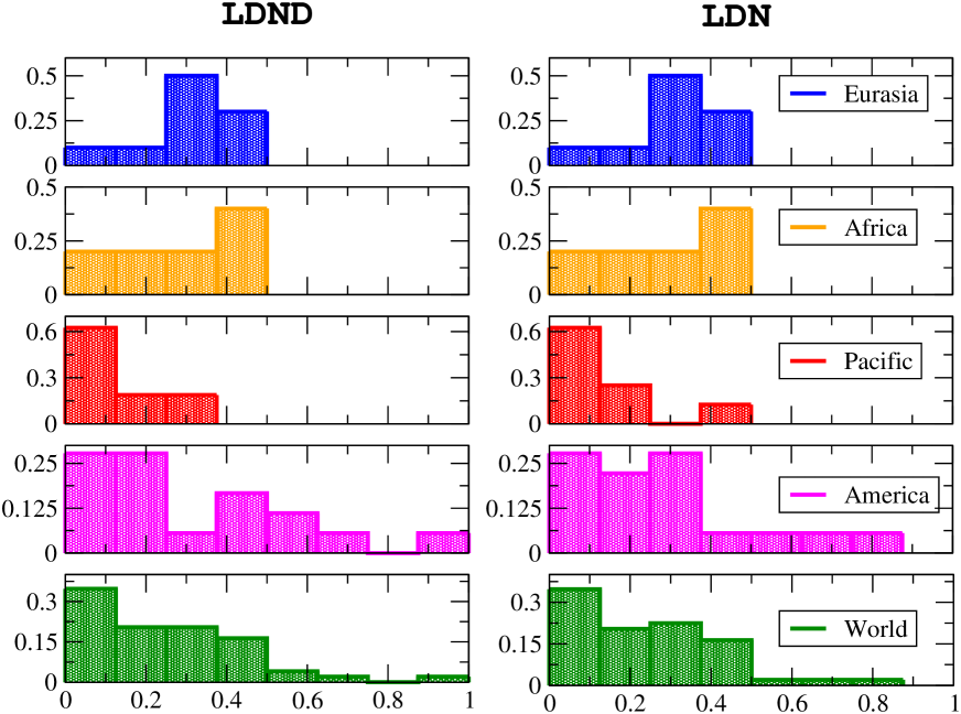
Figure 5: Accuracy histograms as measured with the Generalized Robinson-Foulds score (GRF). For each continent and for the whole world we report the histograms of the GRF as measured over all the families spread on each specific region. We considered here only the FastSBiX algorithm that features slightly better performances with respect to the competing algorithms, and both the LDN (2) (right panel) and the LDND (4) (left panel) definition of distance. The histograms are always peaked near zero, meaning that the rate of errors are always very low, but the variances are quite large. These distributions do not discriminate the performances of the inference using LDN (2) or LDND (4) definition of distances.

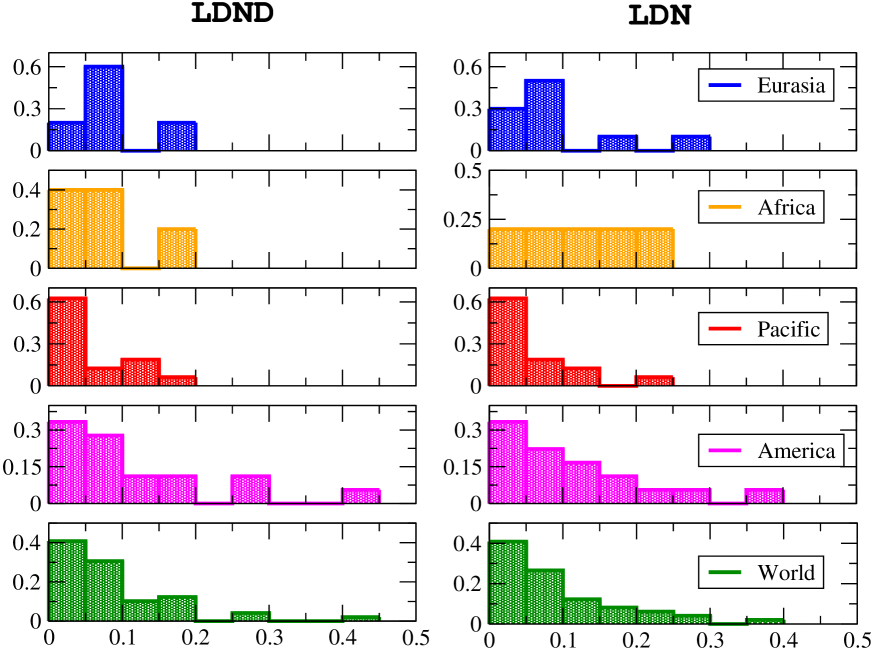
Figure 6: Accuracy histograms as measured with the Generalized Quartet Distance (GQD). For each continent and for the whole world we report the histograms of the GQD as measured over all the families spread on each specific region. We considered here only the FastSBiX algorithm that features slightly better performances with respect to the competing algorithms, both with the LDN (2) (right panel) and the LDND (4) (left panel) definition of distance. The histograms are always peaked near zero, meaning that the rate of errors are always very low. The distributions of the LDN-inferred trees, moreover, display larger variances than the LDND ones, this means that the latter definition allows for better performances in inferring languages trees with a distance-based approach. The overall variances are smaller with respect to the ones in fig. 5.

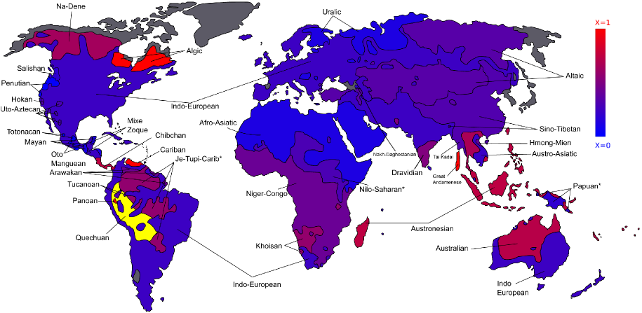
Figure 7: Worldwide accuracy of the inferred language trees. This map represents the level of accuracy of the FastSBiX algorithm on several language families throughout the world. The colors code the values of the Generalized Quartet Distance (GQD) between the trees inferred with the FastSBiX algorithm and the LDND definition of distance for each language family included in the ASJP database and the corresponding Ethnologue classifications. The GQD is normalized with the corresponding random value (see text for details). On the one hand blue regions corresponds to language families for which the inferred trees strongly agree with the Ethnologue classification. On the other hand red regions corresponds to poorly reconstructed language families. Yellow is for the families in which a random reconstruction would get a GQD score of zero, meaning that the Ethnologue classification has a null resolution (the corresponding tree is a star). Grey areas are those for which no data are present in the databases adopted for the reconstruction. Asterisks are for regions which include more than one family of languages. See the Supporting Information for the analogous maps obtained with different algorithms and different definitions of the distance between languages.

Effect of the database completeness and coverage

In this section we consider how the length and the completeness of the lists of words affect the accuracy of the reconstruction. To this end, we restrict our analysis to the Austronesian family for which two different databases are available: the Automated Systematic Judgement Program (ASJP) and the Austronesian Basic Vocabulary Database (ABVD). The two databases mainly differ in two features: ASJP’s lists include at most $100$ items for each language, while ABVD’s lists includes up to $210$ words. In both cases, not all the languages in the family express all the meanings. As we have already pointed out in fig. 2, while in the ASJP there are $40$ words shared by all the languages an additional $60$ words contained only in a small subset, in the ABVD database each word is shared at least by $50\%$ of the languages in the family.

In order to get a fair comparison, we isolate a subset of $305$ lists of words corresponding to languages shared by the two databases. The full list of languages is available in the Supporting Information, Table 10. These two classes of lists are used to infer phylogenetic trees of the corresponding languages to be compared with the Ethnologue classifications. Since the results of the previous section did not show a significant difference between the two definitions of distance matrix, here we only use the LDN distance which allows for faster computations. Further, we only consider the FastSBiX algorithm to reconstruct phylogenies, being the one that features slightly better performances, as shown in the previous section.

We start by investigating the effect of the length of the word-lists on the accuracy of the inference of evolutionary relationships among languages. To this end, for each of the two databases, we proceed as follows: for each meaning $i$ we compute the fraction $f_{i}$ of languages which contains a word for $i$. We sort these values in a decreasing order, obtaining a ranked list of words. We then consider different word-lists, obtained in the following way: we start with the $10$ most frequent words and we progressively add a constant number of words following the ranked list.

We compute the dissimilarity matrices by making use of only the reduced lists constructed as above, and we use those matrices as starting point for the reconstruction algorithm (we use the FastSBiX algorithm for all the results discussed below). Fig. 8 reports the Generalized Robinson-Foulds score (left) and the Generalized Quartet Distance (right) between the inferred trees and the corresponding Ethnologue classifications, as a function of the number $M$ of chosen words, for both the AJSP and the ABVD databases. As a general trend, the number of errors decreases when the size of the word-lists considered increases. Though the large improvement of the accuracy occurs by adding the first $40$ or $50$ words, a slow improvement of the accuracy is always there if one keeps increasing the word-list size. This already points in the direction that, in order to improve the accuracy of the phylogenetic reconstruction, one has to increase the size of the word-lists. The accuracy obtained with the ABVD and ASJP databases are very similar when considering the first $M=40$ most shared words. Upon increasing $M$, ASJP does not feature any improvement while ABVD keeps improving its accuracy, although very slowly, when $M>40$. A possible explanation for this could be related to the presence, in the ASJP database, of meanings with a very low level of sharing (see inset of the left panel of Fig. 8 as well as Fig. 2).

Figure 8: Role of the word-list completeness and coverage. (left) the Generalized Robinson-Foulds (GRF) score between the inferred trees and the corresponding Ethnologue classification for the Austronesian family, vs. the number $M$ of most shared words, both for the ASJP and the ABVD databases. The inset reports the behaviour of $M_{eff}$, the effective number of most shared words, defines as follows. For each list $M_{eff}$ is the sum of all the value of $f_{i}$ for all the meanings in the list. In this way $M_{eff}$ quantifies the effective number of most shared meanings. There is a strong correlation between $M$ and $M_{eff}$ for $M<40$. For $M>40$ $M_{eff}$ does not increase anymore in the ASJP database. This explains why the GRF does not decrease for $M>40$ for the ASJP database. (right) the Generalized Quartet Distance (GQD) between the inferred trees and the corresponding Ethnologue classification for the Austronesian family, vs. the number $M$ of most shared words, both for the ASJP and the ABVD databases. The inset reports the behaviour of the Coverage, which measures the degree of alignment of the word-lists for the different languages considered, vs. $M$ (see text for details about the definition of Coverage). Again there is a strong correlation between the Coverage and $M$. The distance-based algorithm used is FastSBiX with the LDN definition of distance.

The value of $M_{eff}$ (see inset of the left panel of Fig. 8) takes into account in how many languages a given meaning is expressed through a word. The missing information concerns whether pairs of languages have words for the same meaning. Suppose two languages have words for the same number of meanings. This does not mean that the meaning expressed by words in each language are the same. If paradoxically the sets of meanings covered by the two languages had a null overlap, we wouldn’t have data to construct distance matrices. It is thus interesting to measure the degree of overlap between the list of words of pairs of languages. To this end, we define each language $i$ as a binary vector $\vec{l_{i}}$ whose generic entry $l_{i}^{a}$ is $1$ if a word exists in that language for the meaning $a$ and $0$ otherwise. The overlap of two languages $l_{i}$ and $l_{j}$ is thus given by $\sum_{a}l_{i}^{a}l_{j}^{a}$. We define as level of coverage for a database the average overlap between all pairs of languages:

$$\mathrm{Coverage}=\frac{2}{N(N-1)}\sum_{i\neq j}\sum_{a}l_{i}^{a}l_{j}^{a},$$ (10)

where $N$ is the total number of languages considered, the index $a$ runs over all the meanings while the indices $i$ and $j$ run over the different languages. In this way the maximal value of the coverage is given by the total number of meanings $M$ we are considering. The inset of the right panel of Figure 8 reports the curves for the Coverage as a function of $M$. It is evident a strong correlation between $M$ and the Coverage both in the ASJP and ABVD databases. Notice that the maximal observed values of the coverage are well below the theoretical maximum ($100$) in the ASJP database and below the maximum ($210$) in the ABVD database.

The above results can be summarized by saying that the accuracy of the reconstructions strongly depends on the completeness (quantified by $M_{eff}$) as well as on the level of Coverage of the database considered. In the ASJP and ABVD databases $M$, $M_{eff}$ and the Coverage are strongly correlated and one observes a first substantial improvement of the accuracy for $M<40$ and a continuous, though slower, improvement for $M>40$ in the ABVD database, where $M_{eff}$ and the Coverage keeps increasing with $M$.

Discussion

In this work we presented a quantitative investigation of the accuracy of distance-based methods in recovering evolutionary relations between languages. The quantification of the accuracy rests upon the computation of suitable distances between the inferred trees and the classifications made by experts (in our case the Ethnologue).

We introduced two generalized scores, the Generalized Robinson-Foulds score (GRF) and the Generalized Quartet Distance (GQD), which successfully allow for the comparison of binary trees and expert classifications. The generalizations were made necessary in order to take into account the biases due to the presence of non-binary nodes in the Ethnologue classifications, which came from a non fine-grained groupings of the languages. Our scores do not count every refinement as an error, while properly take in account every displacement of a language or wrong groupings with respect to the classifications. These scores are generalizations of standard measures; on the one hand the RF, which is a good measure if we are interested in measuring how far displaced pairs of subtrees have been moved around in one tree compared to another; on the other hand the QD is a more adequate measure whenever it is important to quantify the size of displaced subtrees. Our generalized scores inherit all these properties. Moreover, while in the GRF the stress is on the inferred trees, counting the percentage of wrong bipartitions in the reconstructed tree, in the GQD the stress is on the classification, since we are computing the percentage of correctly inferred quartets in the reconstructed tree.

Once properly defined the tools for the comparison, we conducted a thorough evalution of the accuracy of distance based methods on all the language families listed in the ASJP database. The analysis was carried out by adopting state-of-the art distance-based algorithms as well as two different definitions of distance between lists of words, the LDN (2) and the LDND (4). In all the cases we obtained very robust results, which enabled us to draw some general conclusions. The two different definitions of distances between word-lists, LDN and LDND, almost guarantee the same accuracy for the inference of the trees of languages, as shown in tables 6, 7, 8, 9, with the LDND definition allowing for a slightly better accuracy. The LDN, on the other hand, because of its lower computational complexity, allows for faster computations without a considerable loss of accuracy. The length of the lists used to compute the distances between the languages strongly affects the accuracy of the reconstruction. The comparison between the two databases for the Austronesian family, the ASJP [27] and the ABVD [28] provides very important hints. The accuracy of the reconstruction always worsens if words with a low level of sharing are included; from this perspective it is always better to restrict the analysis to the meanings with an high Coverage instead of using all of them.

Fig. 7 summarizes the accuracy of distance-based reconstruction algorithms for the different language families on the world map. It is evident how at present the accuracy is satisfactory though highly heterogeneous across the different language families. Once the obvious bias is removed due to the finite Ethnologue resolution power, this heterogeneity has to be presumably ascribed to a non homogeneous level of completeness and coverage of the word-lists for specific language families.

In conclusion we provided the first extensive account of the accuracy of distance-based phylogenetic algorithms applied to the recontruction of worldwide language trees. The overall analysis shows as the effort devoted so far to the compilation of large-scale linguistic databases [27, 28] already allows for very good reconstructions. We hope our survey could be an important starting point for further progress in the field, especially for language families for which the available databases are still incomplete or the corresponding Ethnologue classification still poorly resolved.

1 Supporting Information

1.1 Analysis of ASJP database and trees inference

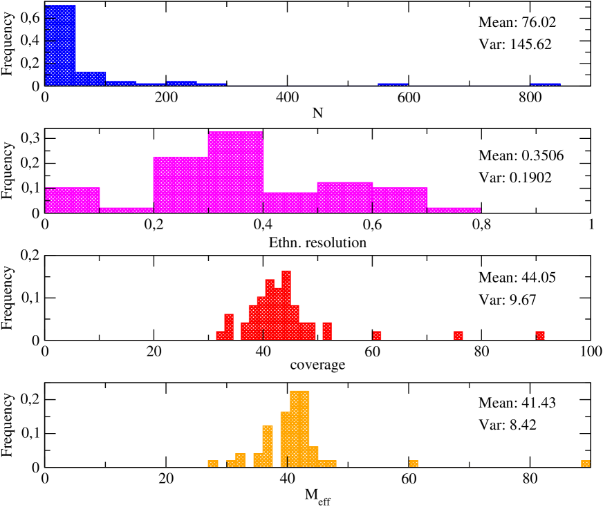
Figure 9: Histograms of ASJP and Ethnologue features. Histograms of the number $N$ of languages in each family, the Ethnologue resolution for each family, $M_{eff}$ and the Coverage of the words lists in each family are reported. While both $N$ and the Ethnologue resolution feature a great variability across the world family, $M_{eff}$ and the Coverage are almost constant in the lists of words related to language families in the ASJP database.

Here we discuss in details some quantitative features of the ASJP and Ethnologue databases. Table 3 summarizes, for each language family in the ASJP database, the number $N$ of languages, the corresponding resolution (as defined below) of the Ethnologue classification, and two properties of words lists discussed in the main text: $M_{eff}$ and the Coverage. Histograms showing the distribution across all the language families of the same quantities are shown in figure 9. We note that, while $M_{eff}$ and Coverage are nearly constant for all the language families in the ASJP database, the number $N$ of languages and the Ethnologue resolution feature a great variability. We quantify the resolution of the Ethnologue classification as $\frac{I-1}{N-2}$, where $I$ is the number of internal nodes in the classification tree and N is the number of leaves. With this definition, completely unresolved classifications, i.e., star trees, will result in a null resolution, while the resolution is equal to one for complete binary classifications. These are the values shown with a color code in Fig. 1 in the main text.

For the sake of completeness, we recall the definition of $M_{eff}$ and Coverage. The former is defined as follows: we name $f_{meaning}$ the fraction of languages in each family which contain a word for $meaning$; $M_{eff}$ is simply the sum of $f_{meaning}$ over all the meanings expressed by a word in at least a language in the considered family. The Coverage is a quantitative measure of the degree of overlap between the lists of words of pairs of languages, defined as:

$$\mathrm{Coverage}=\frac{2}{N(N-1)}\sum_{i\neq j}\sum_{a}l_{i}^{a}l_{j}^{a},$$

where we define each language $i$ as a binary vector $\vec{l_{i}}$, its generic entry $l_{i}^{a}$ being $1$ if a word exists in that language for the meaning $a$ and $0$ otherwise, and the sum is over all pairs of languages in the considered family.

We are now interested in analysing how these quantities affect the phylogeny reconstruction accuracy. To this end, we need to consider how the different measures of misclassification are in turn affected by the characteristics of the databases.

We then consider the accuracy of the inferred trees as measured respectively by the Robinson-Foulds distance, the Quartet Distance, the generalized Robinson-Foulds score and the generalized Quartet Distance. In particular, we investigate how the accuracy of the inferred trees is affected by the quantities considered above, namely the number $N$ of languages in the considered family, the resolution of the corresponding Ethnologue classification, the $M_{eff}$ and the Coverage. In tables 4 and 5 we show the Pearson correlation coefficient (also known as Pearson’s r) between the distance of the inferred trees from the Ethnologue classification, as computed with the different criteria we proposed, and the quantities discussed above. In particular, table 4 shows results obtained considering the whole database while in table 5 we report results obtained by removing from the database those families with null Ethnologue resolution, i.e., for which the Ethnologue tree is a star.

In both cases, we observe a substantial difference between the standard RF and QD measures and their generalizations GRF and GQD. The standard Robinson-Foulds distance features a positive Pearson correlation with the number $N$ of languages in a family, and both the standard Robinson-Foulds distance and Quartet Distance feature a strong negative Pearson correlation with the Ethnologue resolution. Both the GRF and GQD feature a Pearson coefficient with the Ethnologue resolution well below the significance threshold, correcting the biases in the misclassification measure due to lack of information in the Ethnologue database (see main text).

The reconstruction accuracy does not present correlations with $M_{eff}$ and the Coverage, the Pearson coefficient being below the significance threshold for the whole set of measures considered. However, it is important to note that this lack of correlations is actually due to the homogeneity of the ASJP data set with respect to $M_{eff}$ and Coverage. The histograms shown in Fig. 9 for both $M_{eff}$ and Coverage are very peaked, with small variance: this absence of variability does not allow for the detection of correlations between such parameters and the accuracy of the reconstruction. In order to overcome this limitation we performed a comparative analysis of the ASJP and the ABVD databases for the Austronesian family (presented in the main text). The usage of a new database (the ABVD database) allows for the examination of words lists with very different values for both $M_{eff}$ and Coverage, revealing a strong dependence of the accuracy of the phylogenetic inference on such parameters.

In tables 6, 7, 8 and 9 extensive results for the accuracy of the inferred trees, as measured respectively by the Robinson-Foulds distance, the Generalized Robinson-Foulds score, the Quartet Distance and the Generalized Quartet Distance are reported. The Robinson-Foulds distance, as already stressed, is sensitive to the length of the path between two displaced subtrees. Table 6 shows how the reconstruction accuracy as measured by the RF does not depend on the definition of distance matrix (LDN vs. LDND) neither on the specific distance-based algorithm adopted. As stressed in the main text, the use of the standard Robinson-Foulds distance (5) can lead to a systematic larger disagreement due to the presence of non binary internal nodes in Ethnologue trees, i.e., the existence of non fully resolved subgroups of a language family. The generalized Robinson-Foulds score (7) is not affected by this bias. The results obtained with the generalized RF score are shown in table 7. Next we consider the accuracy of the inferred trees as measured by the Quartet Distance. If we take into account the standard definition of the QD (table 8), the accuracy of the inferred trees result quite low, the average distance between the inferred and expert classification being around $45\%$. The adoption of the generalized Quartet Distance score (9) allows to remove the biases due to the presence of star quartets in the classification trees. The generalized QD scores are reported in table 9. The accuracy of the inferred trees in this case turns out to be much higher, with an average fraction of disagreement lower than $10\%$ and with large fluctuations from a minimum of zero to a maximum of roughly $30\%$ for the Panoan family.

1.2 Analysis of ASJP and ABDV databases for the Austronesian Family

We give here some supplementary information about the analysis on the Austronesian Family we presented in the main text. The set of 305 Austronesian languages taken in account is presented in Table 10, the name of languages are the ones shown in http://language.psy.auckland.ac.nz/austronesian/.

The Coverage of the ABVD lists for this set is of $167.32$, for the ASJP is $39.83$. The value of the $M_{eff}$ is $185,23$ for the ABVD database and $46,49$ for the ASJP. The ABVD thus features higher values for both parameters.

In Table 11 we show the distance from the Ethnologue classification, as computed by all the four measures adopted (Robinson-Foulds, Generalized Robinson-Foulds, Quartet-Distance, Generalized Quartet-Distance), of the most accurate tree inferred by using the ABVD list and the most accurate tree inferred by using the ASJP list. The most accurate tree is intended to be the tree, within the ones inferred by the three considered algorithms, that features lower distance from the Ethnologue classification. The LDN definition of distance between languages, which allows for faster computations, has been used here.

All the four tree distances used, point that the inference made by using ABVD lists is more accurate than the one made by the use of ASJP lists: this is a consequence of the higher values of the Coverage and of $M_{eff}$ featured by the ABVD database (see main text). FastSBiX appears again to be the best distance-based algorithm for tree reconstruction, both considering the GRF and GQD distances.

1.3 World maps

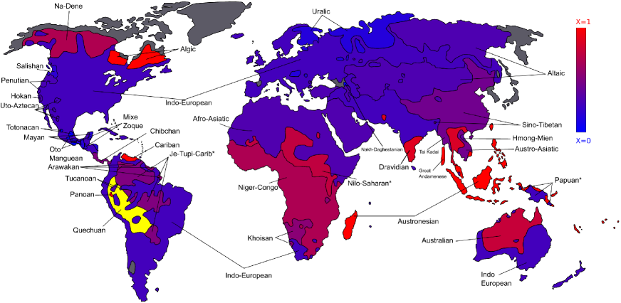
Figure 10: Accuracy of the reconstruction across the planet. NJ, LDN matrix. This map represents the level of accuracy of the Neighbour-Joining algorithm on several language families throughout the world. Trees Inferred with LDN matrices. The legend is the same of Fig.7.

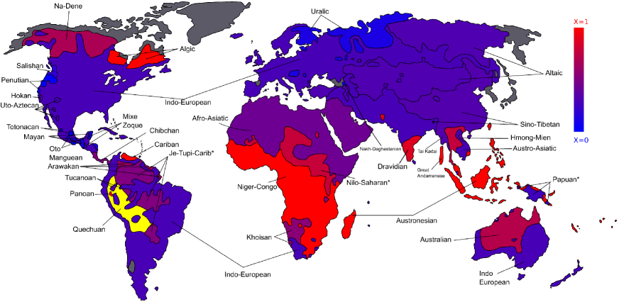
Figure 11: Accuracy of the reconstruction across the planet. FastME, LDN matrix. This map represents the level of accuracy of the FastME algorithm on several language families throughout the world. Trees Inferred with LDN matrices. The legend is the same of Fig.7.

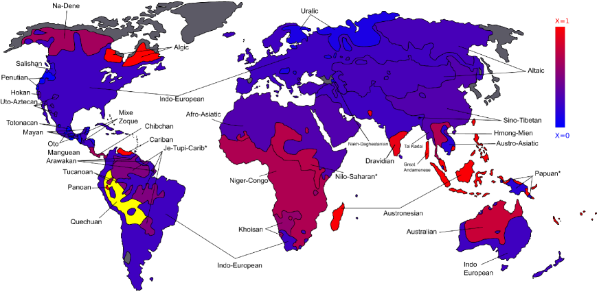
Figure 12: Accuracy of the reconstruction across the planet. FastSBiX, LDN matrix. This map represents the level of accuracy of the Fast-SBiX algorithm on several language families throughout the world. Trees Inferred with LDN matrices. The legend is the same of Fig.7.

We report here world maps showing the Generalized Quartet Distance between inferred trees and Ethnologue classifications. Trees inferred starting from LDN matrices are shown in Fig. 10 (with Neighbour-Joining), Fig. 11 (FastME) and in Fig. 12. Trees inferred starting from LDND matrices are shown in Fig. 13 (Neighbour-Joining), Fig. 11 (FastME). In the main text we have shown the map of the LDND-inferred trees with FastSBiX. We recall that the colors code, for each family $f$, the following quantity $X_{f}=2*GQD(f)/GQD_{random}(f)$, where $GQD_{random}(f)$ represents the value of the GQD obtained as average over $10$ random trees with the same number of leaves (languages) of the family $f$ (see main text). $X_{f}$ quantifies the level of accuracy of the reconstruction with respect to a null model. Blue families are those for which the accuracy is very high while for red families the accuracy is very low, i.e., smaller than half the the random value. Yellow regions on the maps are related to (non-significant) families with null Ethnologue resolution, for which a random reconstruction would get a null value of the GQD.

The difference of the accuracy of the different algorithms is more evident in some regions such as the whole Africa, the Oceania and the east-Europe, whereas areas such as the whole America do not exhibit big differences in all the maps. This visual analysis immediately reveals the main conclusions we have drawn in the main text. Recalling that darker colors (i.e., color with a higher percentage of blue) point to a better accuracy, we see that the sensible regions always get darker while going from LDN maps to LDND ones. This behaviour reveals a slightly better accuracy achieved with the former definition of distance between lists of words. The effect of the different distance-based algorithms used for the reconstruction is visibly more evident. Neighbour-Joining maps displays more red regions than FastME maps; these sensible regions always get darker when observing FastSBiX maps. This visual analysis, thus, enlightens once again the suitability of the noise-reduction procedure used by FastSBiX to infer the correct topology of language trees.

We finally list all the regions where we included the average statistics of more than one language family: In the Nilo-Saharan region we included Kadugli and Nilo-Saharan; in the Papuan-labelled region we included Bosavi, Eleman, Kiwaian, Sko, Western Fly, Marind, Sepik, West Papuan, Trans-New Guinea, Torricelli, Morehead and Upper Maro Rivers, Lakes Plain, Border, Lower Sepik-Ramu.

Family	N	Ethn. Resolution	Coverage	$M_{Eff}$
Afro-Asiatic	227	0.38	43.07	39.66
Algic	28	0.22	43.93	40.34
Altaic	75	0.31	42.47	41.4
Arawakan	48	0.21	43.73	41.06
Australian	186	0.32	40.29	37.05
Austro-Asiatic	52	0.64	60.27	47.54
Austronesian	833	0.35	43.93	40.1
Border	16	0.14	33.94	32.66
Bosavi	15	0	39.33	39.72
Cariban	19	0.53	44.16	42.4
Chibchan	20	0.31	47.67	43.14
Dravidian	21	0.79	45.05	36.15
Eleman	10	0.63	44.3	41.49
Great Andamanese	10	0.25	38.3	39.91
Hmong-Mien	14	0.25	41	43.08
Hokan	24	0.57	46.22	42.29
Indo-European	210	0.36	43.69	41.16
Kadugli	11	0	41	44
Khoisan	16	0.64	41	42.67
Kiwaian	15	0	39	39.69
Lakes Plain	26	0.21	37.19	35.19
Lower Sepik-Ramu	20	0.5	31.95	28.21
Macro-Ge	24	0.32	48.5	42.72
Marind	32	0.33	34.09	30.79
Mayan	75	0.33	75.03	60.09
Mixe-Zoque	14	0.7	91	89.09
Morehead and Upper Maro Rivers	17	0.7	34	31.79
Na-Dene	22	0.6	46.45	42.42
Nakh-Daghestanian	32	0.43	41	41.29
Niger-Congo	558	0.4	41.34	39.89
Nilo-Saharan	113	0.54	42.07	40.38
Oto-Manguean	60	0.3	43.02	40.73
Panoan	18	0.31	41	42.35
Penutian	21	0.31	52.43	44.29
Quechuan	18	0.06	44.33	42.55
Salishan	12	0.4	51	45.45
Sepik	26	0.25	37.81	36.62
Sino-Tibetan	141	0.35	42.7	41.12
Sko	14	0.33	39	41.57
Tai-Kadai	56	0.31	42.11	40.78
Torricelli	31	0.21	37.06	35.63
Totonacan	14	0.25	41	44.44
Trans-New Guinea	293	0.31	40.02	36.01
Tucanoan	14	0.59	47.32	42.92
Tupian	47	0.24	44.75	41.09
Uralic	23	0.43	48.74	42.71
Uto-Aztecan	81	0.34	45.5	41.37
West Papuan	34	0.22	38.21	36.17
Western Fly	39	0	37.77	37.01

Table 3: Statistical Properties of the families in the ASJP database. In this table we report the number $N$ of languages and the resolution of the Ethnologue classification for each family in the ASJP data set. We also show two statistical properties of the lists of words: the $M_{eff}$ of words and the Coverage. See the text for the definitions.

	N	Ethn. resolution	Coverage	$M_{eff}$
RF - FastME	0.3514	-0.1298	-0.1542	-0.1903
RF - NJ	0.3097	-0.1459	-0.1654	-0.2228
RF - FastSBiX	0.3488	-0.2108	-0.1045	-0.1283
QD - FastME	-0.1458	-0.6704	-0.2605	-0.1066
QD - NJ	-0.1847	-0.6901	-0.2623	-0.1120
QD - FastSBiX	-0.211	-0.6717	-0.2494	-0.0926
GRF - FastME	0.1925	0.3414	0.0453	0.0024
GRF - NJ	0.1829	0.3950	0.0833	0.0512
GRF - FastSBiX	0.1869	0.3543	0.1230	0.0985
GQD - FastME	0.0686	0.1079	-0.0923	-0.0749
GQD - NJ	0.1338	0.1352	-0.0855	-0.0599
GQD - FastSBiX	0.0084	0.1392	-0.0597	-0.0256

Table 4: Pearson’s r between reconstruction accuracy and parameters of ASJP and Ethnologue databases. This table shows the Pearson’s r between the accuracy (as measured by the RF, the QD, the GRF and the GDQ) of the trees inferred with FastSBiX, FastME and Neighbour-Joining, starting from the LDND matrices, and different properties of the lists of words of each family in the ASJP database. In particular, we compute the Pearson’s r between the estimated accuracy of the inferred trees and the number $N$ of languages in a family (first column), the Ethnologue Resolution (second column), the Coverage of words in lists (third column) and the effective length of the word-lists $M_{eff}$ (last column).

	N	Ethn. resolution	Coverage	$M_{eff}$
RF - FastME	0.3593	-0.1370	-0.1497	-0.1837
RF - NJ	0.3155	-0.1651	-0.1624	-0.2171
RF - FastSBiX	0.3604	-0.2213	0.0959	-0.1203
QD - FastME	-0.0715	-0.4126	-0.2459	-0.1231
QD - NJ	-0.1309	-0.4476	-0.2499	-0.1322
QD - FastSBiX	-0.1713	-0.4132	-0.1022	-0.1023
GRF - FastME	0.1542	0.1403	-0.0078	-0.0120
GRF - NJ	0.1445	0.2216	0.0355	0.0415
GRF - FastSBiX	0.1482	0.1591	0.0780	0.0931
GQD - FastME	0.0285	-0.1111	-0.1433	-0.0907
GQD - NJ	0.0994	-0.0636	-0.1334	-0.0740
GQD - FastSBiX	-0.0321	-0.0511	0.0883	-0.0374
GQD/GQDrandom - FastME	0.1127	-0.1192	-0.1507	-0.0990
GQD/GQDrandom - NJ	0.1969	-0.0724	-0.1394	-0.0821
GQD/GQDrandom - FastSBiX	0.0348	-0.0576	0.0746	-0.0445
GRF/GRFrandom - FastME	0.1157	0.0779	-0.0391	-0.0229
GRF/GRFrandom - NJ	0.1084	0.1610	0.0026	0.0276
GRF/GRFrandom - FastSBiX	0.1097	0.0994	0.0434	0.0782

Table 5: Pearson’s r between reconstruction accuracy and parameters of ASJP and Ethnologue databases. We show here the same quantities as in table 4, but the correlations are now computed without taking in account families in which the Ethnologue database does not provide a classification (it results in a star tree). Here, the measures $GQD/GQD_{\mathrm{random}}$ and $GRF/GRF_{\mathrm{random}}$ are also taken into account. They allow for an analysis of the correlations of the accuracy of the inference with respect to a null model. Correlations are still very low for all the considered quantities, FastSBiX revealing for all of them the lowest correlation.

ROBINSON-FOULDS DISTANCE
	LDN			LDND
	Neighbour-Joining	FastME	FastSBiX	Neighbour-Joining	FastME	FastSBiX	RANDOM
AFRICA
Khoisan	0.4688	0.4688	0.4688	0.4688	0.4688	0.4688	0.9905
Niger-Congo	0.4964	0.4946	0.4910	0.5000	0.5018	0.4964	0.9995
Nilo-Saharan	0.4292	0.4292	0.4027	0.4204	0.4027	0.3938	0.9952
Kadugli	0.3636	0.3636	0.3636	0.3636	0.3636	0.3636	1.0000
Afro-Asiatic	0.4626	0.4537	0.4537	0.4626	0.4449	0.4449	0.9994
EURASIA
Indo-European	0.5500	0.5310	0.5405	0.5500	0.5357	0.5405	1.0000
Uralic	0.3696	0.3696	0.3696	0.3696	0.3696	0.3261	0.9862
Altaic	0.5400	0.5400	0.5400	0.5400	0.5400	0.5533	0.9979
Dravidian	0.5000	0.5000	0.3571	0.4524	0.4524	0.3571	0.9879
Nakh-Daghestanian	0.2813	0.2813	0.2813	0.2813	0.2813	0.2813	1.0000
Sino-Tibetan	0.5390	0.5248	0.5177	0.5390	0.5177	0.5177	0.9989
Hmong-Mien	0.3571	0.3571	0.3571	0.3571	0.3571	0.3571	1.0000
Tai-Kadai	0.4911	0.4911	0.4911	0.4911	0.4911	0.4911	1.0000
Great Andamanese	0.4000	0.4000	0.4000	0.4000	0.4000	0.4000	1.0000
Austro-Asiatic	0.3462	0.3462	0.3654	0.3269	0.3462	0.3654	0.9975
PACIFIC
Austronesian	0.5258	0.5563	0.5258	0.5246	0.5330	0.5246	0.9994
Border	0.4375	0.4375	0.3750	0.4375	0.4375	0.3750	1.0000
Bosavi	0.4000	0.4000	0.4000	0.4000	0.4000	0.4000	1.0000
Kiwaian	0.4000	0.4000	0.4000	0.4000	0.4000	0.4000	1.0000
Eleman	0.1000	0.1000	0.1000	0.1000	0.1000	0.1000	0.9333
Lower Sepik-Ramu	0.2000	0.2500	0.2000	0.2500	0.2500	0.2000	0.9923
Lakes Plain	0.4231	0.4231	0.4231	0.4231	0.4231	0.4231	0.9929
Marind	0.3438	0.3438	0.3438	0.3438	0.3438	0.3438	0.9947
Morehead and Upper Maro Rivers	0.3235	0.3235	0.3235	0.3235	0.3235	0.3235	1.0000
Sepik	0.4038	0.3654	0.3654	0.3654	0.3269	0.3654	1.0000
Sko	0.1429	0.1429	0.1429	0.1429	0.1429	0.1429	0.9667
Australian	0.4113	0.4274	0.4220	0.4113	0.4274	0.4167	1.0000
Torricelli	0.4839	0.4839	0.4839	0.4516	0.4516	0.4839	1.0000
Trans-New Guinea	0.4454	0.4386	0.4420	0.4386	0.4386	0.4386	0.9995
Western Fly	0.4615	0.4615	0.4615	0.4615	0.4615	0.4615	1.0000
West Papuan	0.4706	0.4412	0.4118	0.4706	0.4412	0.4412	1.0000
AMERICA
Na-Dene	0.5455	0.5000	0.4545	0.5455	0.5000	0.4545	0.9933
Uto-Aztecan	0.1914	0.1914	0.1914	0.1914	0.1790	0.1914	0.9959
Algic	0.5000	0.5000	0.5000	0.4643	0.5000	0.5000	1.0000
Panoan	0.5000	0.5000	0.5000	0.5000	0.5000	0.5000	1.0000
Salishan	0.2917	0.2917	0.2917	0.2917	0.2917	0.2917	1.0000
Quechuan	0.4167	0.4167	0.4167	0.4167	0.4167	0.4167	1.0000
Penutian	0.2619	0.2143	0.2143	0.2619	0.2143	0.2143	0.9931
Tupian	0.4681	0.4681	0.4681	0.4681	0.4681	0.4681	1.0000
Hokan	0.4375	0.3958	0.3958	0.3958	0.4375	0.3958	1.0000
Macro-Ge	0.4583	0.4583	0.5000	0.5000	0.4583	0.5000	1.0000
Oto-Manguean	0.3583	0.3583	0.3583	0.3583	0.3583	0.3583	0.9945
Tucanoan	0.4286	0.4286	0.4286	0.3571	0.4286	0.4286	0.9923
Arawakan	0.4375	0.4375	0.4375	0.4375	0.4375	0.4167	1.0000
Cariban	0.5263	0.5263	0.4737	0.5263	0.5789	0.5263	0.9833
Mixe-Zoque	0.1786	0.2500	0.2500	0.1786	0.2500	0.2500	0.9867
Mayan	0.4600	0.4067	0.4333	0.4467	0.4067	0.4333	1.0000
Chibchan	0.3500	0.3500	0.3500	0.4000	0.4000	0.4000	0.9900
Totonacan	0.2143	0.2143	0.2143	0.2143	0.2143	0.2143	1.0000
AVERAGE	0.3998	0.3970	0.3898	0.3963	0.3962	0.3910	0.9951

Table 6: Robinson-Foulds distance between inferred trees and the Ethnologue classification. This table shows the Robinson-Foulds distances between the inferred trees and the Ethnologue classification for each language family in the ASJP database. For each language family we report the RF distance obtained using both the LDN (2) and the LDND (4) distances between languages in the framework of the NJ, FastMe and FastSBiX algorithms. Finally the last column reports the results obtained in the comparison of the Ethnologue classifications with specific artificial random trees for each language family. First of all the RF distances for the actual inferred trees are much smaller than the corresponding random case. Still these values are always very high independently on the matrix distance used and of the specific phylogenetic algorithm adopted. A systematic effect that increases the errors is the bias induced by the non-binary nodes in the Ethnologue trees.

GENERALIZED ROBINSON-FOULDS SCORE
	LDN			LDND
	Neighbour-Joining	FastME	FastSBiX	Neighbour-Joining	FastME	FastSBiX	RANDOM
AFRICA
Khoisan	0.4615	0.4615	0.4615	0.4615	0.4615	0.4615	0.9769
Niger-Congo	0.4127	0.3891	0.4091	0.4109	0.4018	0.4127	0.9911
Nilo-Saharan	0.3119	0.3395	0.2844	0.3028	0.2844	0.2752	0.9853
Kadugli	0.0000	0.0000	0.0000	0.0000	0.0000	0.0000	0.0000
Afro-Asiatic	0.2500	0.2325	0.2193	0.2544	0.2237	0.2149	0.9908
EURASIA
Indo-European	0.3505	0.3411	0.3224	0.3411	0.3271	0.3084	0.9785
Uralic	0.1500	0.1500	0.1500	0.1500	0.1500	0.1500	0.9450
Altaic	0.3108	0.3108	0.3243	0.3108	0.3108	0.3378	0.9527
Dravidian	0.6111	0.6111	0.4444	0.5556	0.5556	0.3889	0.9889
Nakh-Daghestanian	0.0690	0.0690	0.0690	0.0690	0.0690	0.1034	0.9655
Sino-Tibetan	0.4348	0.4275	0.4130	0.4348	0.4130	0.4130	0.9841
Hmong-Mien	0.1818	0.1818	0.2727	0.2727	0.1818	0.2727	0.8636
Tai-Kadai	0.4118	0.3922	0.4118	0.4118	0.3922	0.4118	0.9725
Great Andamanese	0.2857	0.2857	0.2857	0.2857	0.2857	0.2857	0.4143
Austro-Asiatic	0.3469	0.3469	0.3061	0.2245	0.2449	0.3265	0.9980
PACIFIC
Austronesian	0.3881	0.4063	0.3820	0.3844	0.3942	0.3723	0.9793
Border	0.0769	0.0769	0.0000	0.0769	0.0769	0.0000	0.7538
Bosavi	0.0000	0.0000	0.0000	0.0000	0.0000	0.0000	0.0000
Kiwaian	0.0000	0.0000	0.0000	0.0000	0.0000	0.0000	0.0000
Eleman	0.0000	0.0000	0.0000	0.0000	0.0000	0.0000	0.8429
Lower Sepik-Ramu	0.0000	0.1176	0.0000	0.0588	0.0588	0.0000	0.9765
Lakes Plain	0.1739	0.1739	0.1739	0.1739	0.1739	0.1739	0.9043
Marind	0.0690	0.0690	0.0690	0.0690	0.0690	0.0690	0.9517
Morehead and Upper Maro Rivers	0.1429	0.1429	0.1429	0.0714	0.1429	0.0714	0.9500
Sepik	0.0870	0.0435	0.0435	0.0435	0.0000	0.0435	0.9391
Sko	0.0000	0.0000	0.0000	0.0000	0.0000	0.0000	0.5600
Australian	0.3653	0.4012	0.3772	0.3832	0.3892	0.3653	0.9934
Torricelli	0.2143	0.2500	0.2143	0.2143	0.1786	0.2500	0.9000
Trans-New Guinea	0.2544	0.2230	0.2474	0.2195	0.2404	0.2265	0.9868
Western Fly	0.0000	0.0000	0.0000	0.0000	0.0000	0.0000	0.0000
West Papuan	0.1935	0.1290	0.0968	0.2258	0.1613	0.1613	0.9129
AMERICA
Na-Dene	0.7368	0.6316	0.5789	0.7368	0.6316	0.5789	0.9842
Uto-Aztecan	0.1622	0.1622	0.1622	0.1622	0.1351	0.1892	0.9405
Algic	0.3846	0.3846	0.3462	0.3846	0.3846	0.3462	0.9385
Panoan	0.8000	0.8000	0.7333	0.8000	0.8000	0.7333	0.9800
Salishan	0.1111	0.1111	0.1111	0.1111	0.1111	0.1111	0.9556
Quechuan	0.0000	0.0000	0.0000	0.0000	0.0000	0.0000	0.0000
Penutian	0.1667	0.0556	0.0556	0.1111	0.0556	0.0556	0.9667
Tupian	0.4444	0.4000	0.4222	0.3556	0.4667	0.4667	0.9867
Hokan	0.4000	0.3500	0.3500	0.3500	0.4500	0.4000	0.9800
Macro-Ge	0.3810	0.3810	0.3333	0.3810	0.3333	0.3810	0.9333
Oto-Manguean	0.0357	0.0357	0.0357	0.0357	0.0357	0.0357	0.9393
Tucanoan	0.1875	0.1875	0.2500	0.1250	0.1875	0.1875	0.9625
Arawakan	0.2195	0.1951	0.1951	0.2195	0.1951	0.1707	0.9463
Cariban	0.8125	0.7500	0.7500	0.7500	0.8750	0.8750	0.9500
Mixe-Zoque	0.1111	0.2222	0.2222	0.1111	0.2222	0.2222	0.9889
Mayan	0.1972	0.1268	0.1549	0.1831	0.1268	0.1549	0.9394
Chibchan	0.4000	0.4000	0.3333	0.5333	0.5333	0.5333	0.9600
Totonacan	0.0000	0.0000	0.0000	0.0000	0.0000	0.0000	0.7571
AVERAGE	0.2470	0.2401	0.2276	0.2399	0.2394	0.2354	0.8320

Table 7: Generalized Robinson-Foulds scores between inferred trees and the Ethnologue classification. This table shows the generalized Robinson-Foulds scores between the inferred trees and the Ethnologue classification. The legend is the same as in Table 6. The generalization has been introduced to get rid of biases in the Robinson-Foulds distance, due to the presence of non binary nodes in the classifications trees. The average scores are now much smaller (roughly for a factor $2$) than for the usual Robinson-Foulds distance.

QUARTET DISTANCE
	LDN			LDND
	Neighbour-Joining	FastME	FastSBiX	Neighbour-Joining	FastME	FastSBiX	RANDOM
AFRICA
Khoisan	0.2885	0.2885	0.2984	0.2885	0.2885	0.2984	0.7088
Niger-Congo	0.3396	0.5057	0.3401	0.3471	0.3355	0.2853	0.6120
Nilo-Saharan	0.3420	0.3484	0.3311	0.2141	0.2214	0.2128	0.6912
Kadugli	1.0000	1.0000	1.0000	1.0000	1.0000	1.0000	1.0000
Afro-Asiatic	0.2550	0.2808	0.2556	0.2508	0.2371	0.2083	0.6440
EURASIA
Indo-European	0.1694	0.1743	0.1661	0.1650	0.1632	0.1626	0.6065
Uralic	0.5007	0.4949	0.4949	0.5007	0.4949	0.4963	0.8087
Altaic	0.2800	0.2813	0.2733	0.2800	0.2813	0.2891	0.7167
Dravidian	0.3666	0.3666	0.3793	0.3101	0.3078	0.2526	0.7095
Nakh-Daghestanian	0.2613	0.2613	0.2613	0.2613	0.2613	0.2969	0.7455
Sino-Tibetan	0.5051	0.4829	0.4828	0.4900	0.4907	0.4821	0.7879
Hmong-Mien	0.4016	0.4016	0.4066	0.4066	0.4016	0.4066	0.7690
Tai-Kadai	0.3772	0.3523	0.3300	0.3701	0.3523	0.3245	0.7093
Great Andamanese	0.9571	0.9571	0.9571	0.9571	0.9571	0.9571	0.9805
Austro-Asiatic	0.3336	0.2923	0.2593	0.2549	0.2558	0.2763	0.7381
PACIFIC
Austronesian	0.3731	0.3721	0.3306	0.2963	0.3976	0.2746	0.6650
Border	0.6269	0.6269	0.5692	0.6269	0.6269	0.5692	0.8344
Bosavi	1.0000	1.0000	1.0000	1.0000	1.0000	1.0000	1.0000
Kiwaian	1.0000	1.0000	1.0000	1.0000	1.0000	1.0000	1.0000
Eleman	0.1190	0.1190	0.1190	0.1190	0.1190	0.1190	0.6895
Lower Sepik-Ramu	0.1969	0.2140	0.1969	0.2004	0.2004	0.1969	0.7354
Lakes Plain	0.4813	0.4813	0.4813	0.4813	0.4813	0.4813	0.7817
Marind	0.2000	0.2000	0.2000	0.2000	0.2000	0.2000	0.7345
Morehead and Upper Maro Rivers	0.2664	0.3496	0.2664	0.3345	0.3546	0.3345	0.7282
Sepik	0.3466	0.3523	0.3145	0.3451	0.3130	0.3451	0.7738
Sko	0.4857	0.4857	0.4857	0.4857	0.4857	0.4857	0.7571
Australian	0.5674	0.5553	0.5685	0.5792	0.5666	0.5573	0.7824
Torricelli	0.4898	0.4625	0.4625	0.4513	0.4493	0.4625	0.8037
Trans-New Guinea	0.4593	0.4592	0.4527	0.4532	0.4474	0.4505	0.7265
Western Fly	1.0000	1.0000	1.0000	1.0000	1.0000	1.0000	1.0000
West Papuan	0.2529	0.2455	0.2209	0.2471	0.2397	0.2397	0.7309
AMERICA
Na-Dene	0.3794	0.3753	0.3671	0.3794	0.3753	0.3671	0.7234
Uto-Aztecan	0.2914	0.2914	0.2914	0.2914	0.2945	0.2965	0.7419
Algic	0.5673	0.5673	0.5695	0.5885	0.5941	0.5782	0.7717
Panoan	0.6876	0.6909	0.6791	0.6928	0.6909	0.6827	0.8152
Salishan	0.3354	0.3354	0.3354	0.3354	0.3354	0.3354	0.7578
Quechuan	1.0000	1.0000	1.0000	1.0000	1.0000	1.0000	1.0000
Penutian	0.2145	0.1370	0.1370	0.2092	0.1370	0.1370	0.7068
Tupian	0.5359	0.5188	0.5109	0.5055	0.5135	0.5209	0.8169
Hokan	0.2577	0.2582	0.2690	0.2447	0.2733	0.2654	0.7255
Macro-Ge	0.4343	0.4551	0.4650	0.4789	0.4645	0.4823	0.7764
Oto-Manguean	0.3767	0.3767	0.3767	0.3767	0.3767	0.3767	0.7855
Tucanoan	0.2608	0.2608	0.3351	0.2567	0.2608	0.2608	0.7166
Arawakan	0.3494	0.3685	0.3212	0.3541	0.3685	0.3133	0.7363
Cariban	0.6370	0.5986	0.5929	0.5815	0.6391	0.6373	0.7304
Mixe-Zoque	0.2384	0.2566	0.2566	0.2384	0.2566	0.2566	0.7402
Mayan	0.2060	0.1925	0.1943	0.2057	0.1925	0.1943	0.7074
Chibchan	0.5788	0.5788	0.6023	0.6199	0.6199	0.6199	0.8291
Totonacan	0.7000	0.7000	0.7000	0.7000	0.7000	0.7000	0.9224
AVERAGE	0.4550	0.4566	0.4471	0.4485	0.4494	0.4426	0.7744

Table 8: Quartet Distance between inferred trees and the Ethnologue classification. This table shows the Quartet Distance between the inferred trees and the Ethnologue classification for each language family in the ASJP database. The legend is the same as in Table 6. In this case the scores are affected by the presence of star quartets of taxa in the Ethnologue trees, as a consequence of the existence of non-binary nodes.

GENERALIZED QUARTET DISTANCE
	LDN			LDND
	Neighbour-Joining	FastME	FastSBiX	Neighbour-Joining	FastME	FastSBiX	RANDOM
AFRICA
Khoisan	0.1809	0.1809	0.1923	0.1809	0.1809	0.1923	0.6650
Niger-Congo	0.1756	0.3830	0.1763	0.1850	0.1705	0.1078	0.5158
Nilo-Saharan	0.2436	0.2510	0.2310	0.0966	0.1051	0.0951	0.6451
Kadugli	0.0000	0.0000	0.0000	0.0000	0.0000	0.0000	0.0000
Afro-Asiatic	0.0895	0.1209	0.0901	0.0843	0.0676	0.0323	0.5647
EURASIA
Indo-European	0.0738	0.0793	0.0701	0.0689	0.0669	0.0662	0.5609
Uralic	0.0458	0.0347	0.0347	0.0458	0.0347	0.0373	0.6355
Altaic	0.0990	0.1006	0.0906	0.0988	0.1006	0.1102	0.6451
Dravidian	0.2978	0.2978	0.3119	0.2352	0.2327	0.1715	0.6779
Nakh-Daghestanian	0.0179	0.0179	0.0179	0.0179	0.0179	0.0653	0.6632
Sino-Tibetan	0.1411	0.1026	0.1024	0.1149	0.1161	0.1012	0.6319
Hmong-Mien	0.1243	0.1243	0.1316	0.1316	0.1243	0.1316	0.6620
Tai-Kadai	0.2838	0.2553	0.2296	0.2758	0.2553	0.2232	0.6659
Great Andamanese	0.6786	0.6786	0.6786	0.6786	0.6786	0.6786	0.6283
Austro-Asiatic	0.1489	0.0962	0.0542	0.0485	0.0496	0.0757	0.6658
PACIFIC
Austronesian	0.3006	0.2995	0.2523	0.2149	0.3279	0.1907	0.5132
Border	0.1339	0.1339	0.0000	0.1339	0.1339	0.0000	0.6156
Bosavi	0.0000	0.0000	0.0000	0.0000	0.0000	0.0000	0.0000
Kiwaian	0.0000	0.0000	0.0000	0.0000	0.0000	0.0000	0.0000
Eleman	0.0000	0.0000	0.0000	0.0000	0.0000	0.0000	0.5705
Lower Sepik-Ramu	0.0000	0.0213	0.0000	0.0044	0.0044	0.0000	0.6717
Lakes Plain	0.2096	0.2096	0.2096	0.2096	0.2096	0.2096	0.6675
Marind	0.0284	0.0284	0.0284	0.0284	0.0284	0.0284	0.6763
Morehead and Upper Maro Rivers	0.0673	0.1732	0.0673	0.1540	0.1797	0.1540	0.6549
Sepik	0.0490	0.0573	0.0022	0.0468	0.0000	0.0468	0.6716
Sko	0.0000	0.0000	0.0000	0.0000	0.0000	0.0000	0.2714
Australian	0.2405	0.2195	0.2426	0.2614	0.2391	0.2230	0.6182
Torricelli	0.1592	0.1144	0.1144	0.0959	0.0926	0.1144	0.6769
Trans-New Guinea	0.1221	0.1221	0.1114	0.1122	0.1029	0.1078	0.5561
Western Fly	0.0000	0.0000	0.0000	0.0000	0.0000	0.0000	0.0000
West Papuan	0.0714	0.0623	0.0317	0.0642	0.0550	0.0550	0.6654
AMERICA
Na-Dene	0.2251	0.2200	0.2098	0.2251	0.2200	0.2098	0.6548
Uto-Aztecan	0.0911	0.0911	0.0911	0.0911	0.0951	0.0976	0.6686
Algic	0.3609	0.3609	0.3641	0.3920	0.4003	0.3768	0.6628
Panoan	0.4885	0.4937	0.4746	0.4970	0.4937	0.4805	0.6974
Salishan	0.0600	0.0600	0.0600	0.0600	0.0600	0.0600	0.6577
Quechuan	0.0000	0.0000	0.0000	0.0000	0.0000	0.0000	0.0000
Penutian	0.0958	0.0066	0.0066	0.0897	0.0066	0.0066	0.6626
Tupian	0.1783	0.1478	0.1340	0.1244	0.1386	0.1517	0.6757
Hokan	0.1006	0.1012	0.1143	0.0848	0.1195	0.1099	0.6674
Macro-Ge	0.1598	0.1907	0.2052	0.2260	0.2046	0.2310	0.6677
Oto-Manguean	0.0015	0.0015	0.0015	0.0015	0.0015	0.0015	0.6857
Tucanoan	0.1105	0.1105	0.2001	0.1056	0.1105	0.1105	0.6593
Arawakan	0.1859	0.2098	0.1506	0.1916	0.2098	0.1407	0.6702
Cariban	0.5455	0.4973	0.4902	0.4761	0.5480	0.5458	0.6625
Mixe-Zoque	0.0528	0.0754	0.0754	0.0528	0.0754	0.0754	0.6772
Mayan	0.0469	0.0307	0.0327	0.0465	0.0307	0.0327	0.6483
Chibchan	0.1673	0.1673	0.2140	0.2488	0.2488	0.2488	0.6625
Totonacan	0.0000	0.0000	0.0000	0.0000	0.0000	0.0000	0.2224
AVERAGE	0.0984	0.0965	0.0870	0.0884	0.0894	0.0825	0.4122

Table 9: Generalized Quartet Distance between inferred trees and the Ethnologue classification. The generalized QD, shown in this table, quantifies the overall disagreement between inferred trees and the Ethnologue classifications. The legend is the same as in Table 6. The errors are now extremely low being always lower than $10\%$. This means that distance based approaches lead to accurate and robust classifications of the languages taken in account.

Acehnese	Gapapaiwa	Kwara’ae (Solomon Islands’)	Muyuw	Solos
Aklanon-Bisayan	Gaddang	Lahanan	Nalik	Soboyo
Alune	Gayo	Lala	Nanggu	Sowa
Amahai	Gedaged	Lamalera (lembata)	Nauna	Suau
Amara	Geser	Lamboya	Nehan	Sudest
Ambai (Yapen)	Ghari	Lamogai (Mulakaino)	Nengone	Surigaonon
Anakalang	Gorontalo (Hulondalo)	Lampung	Nggao (Poro)	Tabar
Apma Suru Kavian	Gumawana	Langalanga	Nggela	Tagabili
Aputai	Haku	Lau	Nila	Tagalog
Araki (Southwest Santo)	Hawaiian	Leipon	Niue	Tagbanwa, Aborlan Dialect
Arosi (Tawatana Village)	Hiligaynon	Lengo	Nukuoro	Tagbanwa, Kalamian, Coron Island Dialect
As	Hitu (Ambon)	Letinese	Numfor	Tahitian (Modern)
Asumboa	Hiw	Levei	Ogan	Taiof
Bali	Hoava	Likum	Oroha	Takia
Banggai (W.dialect)	Iaai	Lio, Flores Tongah	Paiwan	Talur
Banoni	Iban	Longgu	Palauan	Tanga
Bantik	Ibanag	Loniu	Palu’e (Nitung)	Tarpia
Baree	Idaan	Lou	Pangasinan	Tausug, Jolo Dialect
Barok	Iliun	Luang	Papora	Tawala
Bauro (Baroo Village)	Ilokano	Luangiua	Patpatar	Teanu
Belait	Ilongot;Kakiduge:n	Lunga Lunga (Minigir)	Paulohi	Tela-Masbuar
Besemah	Imorod	Lungga	Pazeh	Teop
Biga (Misool)	Imroing	Maanyan	Penrhyn	Teun
Bilur	Inabaknon	Madak	Perai	Thao
Bima	Indonesian	Madurese	Phan Rang Cham (Eastern Cham)	Tiang
Bintulu	Inibaloi	Magori (South East Papua)	Pukapuka	Tigak
Binukid	Iranun	Maisin	Pulo-Annan	Tikopia
Blablanga	Itneg, Binongan	Malango	Puluwatese	Timugon (Murut)
Bobot	Ivatan, Basco Dialect	Maleu	Puyuma	Tolo
Bolaang Mongondow	Jawe	Mamanwa	Raga	Tongan
Bonerate	Kadorih	Mamboru	Rarotongan	Tonsea
Bonfia	Kahua	Manam	Rejang Rejang	Tontemboan
Bughotu	Kaidipang	Manggarai	Rennellese	Torau
Bukat	Kairiru	Manihiki	Ririo	Tsou
Buli	Kalagan	Manobo, Ata (down river)	Roma	Tugun
Bunun	Kalinga, Limos	Manobo, Dibabawon	Roro	Tunjung
Buol	Kallahan, Keleyqiq	Manobo, Ilianen (Kibudtungan Dialect)	Rotuman	Ubir
Butuanon	Kambera	Manobo, Sarangani, Kayaponga Dialect	Roviana	Ughele
Carolinian	Kanakanabu	Mansaka	Rukai	Ujir (N.Aru)
Cebuano	Kandas	Maori	Rurutuan	Ura
Centra Amis	Kapampangan	Mapun	Sa (south easterndialect)	Uruava
Chamorro	Kapingamarangi	Maranao	Sa’a	Vaeakau-Taumako
Chru	Katingan	Marau	Saaroa	Vaghua
Chuukese (AKA Trukese)	Kaulong (Au Village)	Marovo	Sambal, Botolan	Varisi
Dai	Kavalan	Marshallese	Samoan	Vitu
Dawera-Daweloor	Kayupulau[Kajupulau]	Masiwang	Sangir	Wampar
Dehu	Kazukuru	Matukar	Sasak	Wanukaka
Diodio	Kemak	Maututu	Savu	Waray-Waray
Dorio	Kerinci	Mbaelelea	Seimat	Waropen
Doura	Kilivila	Mbaengguu	Sekar	Watubela
Emae	Kiribati	Mbirao	Selaru	Wedau
Emplawas	Kis	Mekeo	Sengseng	Windesi Wandamen
Ende	Kisar	Mengen	Serili	Wogeo
Erai	Kokota	Minangkabau	Serua	Woleaian
Fagani	Komering	Modang	Siar	Wolio
Fataleka	Kove	Moken	Sika	Wuvulu
Favorlang	Kuni	Molima	Simbo	Yabem
Fijian (Bau)	Kusaghe	Mono	Singhi	Yakan
Futuna-Aniwa	Kusaie	Mota	Siraya	Yamdena
Futuna, East	Kwai	Motu	Soa	Yapese
Gabadi	Kwaio	Nakanai (Bileki Dialect)	Sobei	Zabana (Kia)

Table 10: List of the 305 Austronesian languages considered in both ABVD and ASJP databases. Here we report the complete list of the 305 languages taken in account in our studies of ABVD and ASJP list of words for the Austronesian family. Names of languages are reported as presented in http://language.psy.auckland.ac.nz/austronesian/.

—	ABVD			ASJP
	Neighbour-Joining	FastME	FastSBiX	Neighbour-Joining	FastME	FastSBiX
RF	0.5762	0.5573	0.6240	0.6026	0.5993	0.5993
QD	0.3508	0.3657	0.2371	0.3605	0.4594	0.3163
GRF	0.5464	0.5331	0.5430	0.6192	0.6325	0.5927
GQD	0.2860	0.3024	0.1609	0.2969	0.4055	0.2815

Table 11: Accuracy in reconstructing the Austronesian family tree with the ABVD and ASJP database. This table shows the Robinson-Foulds distance, the Quartet Distance and their generalizations, between the Austronesian language tree (inferred with both the ASJP and the ABVD database) and its relative Ethnologue-Classification for the languages shown in Table.10. In this case we only used the LDN definition of distance between lists of words and FastSBiX as distance-based algorithm to infer the trees. All the measures indicate that the ABVD database allows for a more accurate reconstruction of this language tree.

Figure 13: Accuracy of the reconstruction across the planet. NJ, LDND matrix. This map represents the level of accuracy of the Neighbour-Joining algorithm on several language families throughout the world. Trees Inferred with LDND matrices. The legend is the same of Fig.7.

Figure 14: Accuracy of the reconstruction across the planet. FastME, LDND matrix. This map represents the level of accuracy of the FastME algorithm on several language families throughout the world. Trees Inferred with LDND matrices. The legend is the same of Fig.7.

References

- 1. Renfrew C, McMahon A, Trask L, editors (2000) Time Depth in Historical Linguistics. The McDonald Institute for Archeological Research.
- 2. Joseph BD, Janda RD, editors (204) The handbook of historical linguistics. Blackwell Publishing.
- 3. Wichmann S, Grant AP, editors (2010) Quantitative Approaches to Linguistic Diversity, volume 27 of Special Issue of Diachronica Commemorating the centenary of the birth of Morris Swadesh. John Benjamins Publishing company.
- 4. Kishino H, Thorne JL, Bruno WJ (2001) Performance of a divergence time estimation methods under a probabilistic model of rate of evolution. Mol Biol Evol 18: 352-361.
- 5. Langley CH, Fitch WM (1974) An estimation of the constancy of the rate of molecular evolution. J Mol Evol 3: 161-177.
- 6. Rambaut A, Bromham L (1998) Estimating divergence data from molecular sequences. Mol Biol Evol 15: 442-448.
- 7. Sanderson MJ (2002) A nonparametric approach to estimating divergence times in the absence of rate constancy. Mol Biol Evol 19: 101-109.
- 8. Sanderson MJ (2002) Estimating absolute rates of molecular evolution and divergence times: a penalized likelihood approach. Mol Biol Evol 19: 101-109.
- 9. Thorne JL, Kishino H, Painter IS (1998) Estimating the rate of evolution of the rate of evolution. Mol Biol Evol 15: 1647-1657.
- 10. Gray RD, Atkinson Q (2003) Language-tree divergence times support the anatolian theory of indo-europian origin. Nature 426: 435-439.
- 11. Bryant D, Filimon F, Gray RD (2005) Untangling our past: Languages, trees, splits and networks. In: RMace C, SShennan, editors, The evolution of cultural diversity: phylogenetic approaches, UCL press. pp. 67-84.
- 12. Atkinson PMQ, Meade A (2007) Frequency of word-use predicts rates of lexical evolution throughout indo-european history. Nature 449: 717-720.
- 13. Atkinson Q, Meade A, Venditti C, Greenhill S, Pagel M (2008) Languages evolve in punctuational bursts. Science 319: 588.
- 14. Dunn M, Levinson SC, Lindström E, Reesink G, Terrill A (2008) Structural phylogeny in historical linguistics: Methodological explorations applied in Island Melanesia. Language 84: 710–759.
- 15. Gray RD, Drummond AJ, Greenhill SJ (2009) Language phylogenies reveal expansion pulses and pauses in pacific settlement. Science 323: 479-483.
- 16. Swadesh M (1952) Lexico-statistic dating of prehistoric ethnic contacts. Proceedings of the National American Philosophical Society 96: 453-463.
- 17. Swadesh M (1955) Towards greater accuracy in lexicostatistic dating. International Journal of American Linguistics 21: 121-137.
- 18. Nerbonne J, Heeringa W, Kleiweg P (1999) Comparison and classification of dialects. In: Proceedings of the 9th Meeting of the European Chapter of the Association for Computational Linguistics. pp. 281-282.
- 19. Wichmann S, Holman EW, Bakker D, Brown CH (2010) Evaluating linguistic distance measures. Physica A 389: 3632-3639.
- 20. Petroni F, Serva M (2010) Binary codes capable of correcting deletions, insertions, and reversals. Physica A 389: 2280-2283.
- 21. Pompei S, Caglioti E, Tria F, Loreto V (2010) Distance-based phylogenetic algorithms: new insights and applications. Mathematical Models and Methods in Applied Sciences (M3AS) 20: 1511-1532.
- 22. Tria F, Caglioti E, Loreto V, Pagnani A (2010) A stochastic local search algorithm for distance-based phylogeny reconstruction. Molecular Biology and Evolution 27: 2587-2595.
- 23. Tria F, Caglioti E, Loreto V, Pompei S (2010) A fast noise reduction driven distance-based phylogenetic algorithm. Proceedings of BIOCOMP2010 - The 2010 International Conference on Bioinformatics & Computational Biology .
- 24. Lewis M, editor (2009) Ethnologue: Languages of the World, Sixteenth edition. Dallas, Texas. SIL International. Online version: http://www.ethnologue.com/.
- 25. Robinson D, Foulds L (1981) Comparison of phylogenetic trees. Mathematical Biosciences 53: 131-147.
- 26. Bryant D, Tsang J, Kearney PE, Li M (2000) Computing the quartet distance between evolutionary trees. Proceedings of the Eleventh Annual ACM-SIAM Symposium on Discrete Algorithms : 258-286.
- 27. Holmann EW, Wichmann S, Brown CH, Velupillai V, Muller A, et al. (2008) Explorations in automated language classification. Folia Linguistica 42: 331-354.
- 28. Greenhill SJ, Blust R, Gray RD (2008) The austronesian basic vocabulary database: From bioinformatics to lexomics. Evolutionary Bioinformatics 4: 271-283.
- 29. Serva M, Petroni F (2008) Indo-european languages tree by levenshtein distance. Europhysics Letters 81: 68005.
- 30. Levenshtein VI (1966) Measures of lexical distance between languages. Soviet Physics Doklady 10: 707-710.
- 31. Bakker D, Müller A, Velupillai V, Wichmann S, Brown C, et al. (2009) Adding typology to lexicostatistics: a combined approach to language classification. Linguistic Typology 13: 167-179.
- 32. Christensen C, Mailund T, Pedersen CNS, Randers M (2005) Computing the quartet distance between trees of arbitrary degree. In: Proceedings of the 5th Workshop in Algorithms in Bioinformatics (WABI 2005). Springer, volume 3692 of Lecture Notes in Computer Science, pp. 77-88.
- 33. Randers M (2006) Computing the Quartet Distance Between Trees of Arbitrary Degrees. Master’s thesis, University of Aarhus.
- 34. Saitou N, Nei M (1987) The neighbor-joining method: a new method for reconstructing phylogenetic trees. Mol Biol Evol 4: 406–425.
- 35. Desper R, Gascuel O (2002) Fast and accurate phylogeny reconstruction algorithms based on the minimum-evolution principle. Journal of Computational Biology 9: 687–705.