A New Three-Parameter Correlation for Gamma-ray Bursts with a Plateau Phase in the Afterglow

Abstract

Aims. Gamma ray bursts (GRBs) have great advantages for their huge burst energies, luminosities and high redshifts in probing the Universe. A few interesting luminosity correlations of GRBs have been used to test cosmology models. Especially, for a subsample of long GRBs with known redshifts and a plateau phase in the afterglow, a correlation between the end time of the plateau phase (in the GRB rest frame) and the corresponding X-ray luminosity has been found.

Methods. In this paper, we re-analyze the subsample and found that a significantly tighter correlation exists when we add a third parameter, i.e. the isotropic $\gamma$-ray energy release, into the consideration. We use the Markov chain Monte Carlo techniques to get the best-fit coefficients.

Results. A new three-parameter correlation is found for the GRBs with an obvious plateau phase in the afterglow. The best fit correlation is found to be $L_{\rm X}\propto T_{\rm a}^{-0.87}E_{\gamma,\rm iso}^{0.88}$. Additionally, both long and intermediate duration GRBs are consistent with the same three-parameter correlation equation.

Conclusions. It is argued that the new three-parameter correlation is consistent with the hypothesis that the subsample of GRBs with a plateau phase in the afterglow be associated with the birth of rapidly rotating magnetars, and that the plateau be due to the continuous energy-injection from the magnetar. It is suggested that the newly born millisecond magnetars associated with GRBs might provide a good standard candle in the Universe.

1 Introduction

Gamma-ray busts (GRBs) are one of the most powerful and energetic explosive events in the Universe. The observations of GRBs up to redshifts higher than 8 (Salvaterra et al. 2009; Cucchiara et al. 2011) make GRBs to be among the farthest known astrophysical sources. Taking their considerable event rate into consideration, GRBs may be good candidates that can be used to probe our Universe. Several interesting correlations have been suggested for GRBs (Amati et al. 2002; Norris et al. 2000; Ghirlanda et al. 2004a; Liang & Zhang 2005; Dainotti et al. 2010; Qi & Lu 2010). Based on them, the cosmology parameters have been tentatively constrained (e.g., Fenimore & Ramirez-Ruiz 2000; Schaefer 2003, 2007; Dai et al. 2004; Ghirlanda et al. 2004b, 2006; Amati et al. 2008; Wang & Dai 2006; Dainotti et al. 2008; Wang et al. 2009, 2011).

To derive a meritorious constraint on the cosmology parameters, the most important thing is to find a credible standard candle relation for GRBs. Currently, no such a relation can be established when all GRBs are involved (Butler et al. 2009; Yu et al. 2009). The reason may be that different GRBs should be produced via various mechanisms. Interestingly, for a subsample of long GRBs with known redshifts and with a plateau phase in the afterglow, an anti-correlation has been reported to exist between the end time of the plateau phase ($T_{\rm a}$, measured in the GRB rest frame) and the corresponding X-ray luminosity ($L_{\rm X}$) at that moment (Dainotti et al. 2010, hereafter D2010). In this paper, we call Dainotti et al.’s two parameter correlation as the L-T correlation. The intrinsic scatter of this correlation is still too large to be directly applied as a redshift estimator (Dainotti et al. 2011). Additionally, normal long duration GRBs and the intermediate duration GRBs do not obey the same correlation equation (D2010), and the intermediate class seem to be more scattered in the plot.

In this study, we have tried to add a third parameter, i.e. the isotropic $\gamma$-ray energy release ($E_{\gamma,\rm iso}$), into the correlation. We find that the new three-parameter correlation (designated as the L-T-E correlation) is much tighter than the previous L-T correlation. It is also obeyed by both the long GRBs and the intermediate calss. The L-T-E correlation may hopefully give a better measure for our Universe. In Section 2, we describe our GRB sample and the method of data analysis. Our results are presented in Section 3. Section 4 is our discussion and conclusions.

2 Sample & Data analysis

According to $Swift$ observations, many GRBs show a plateau phase in the early afterglow, prior to the normal power-law decay phase (Zhang et al. 2006; Nousek et al. 2006). In this study, we will mainly concentrate on the GRBs with such a characteristics. All our GRBs are taken from Dainotti et al.’s sample (D2010). In D2010’s data table, totally 77 GRBs are initially included, with known redshift and with a plateau phase in the afterglow light curve. After removing the intermediate class GRBs and some GRBs with relatively large errors, they finally limited their major statics to only 62 long GRBs. Here, we have re-selected the events by taking into account the following three criterions in our studies: (1) the plateau should be obvious (GRBs 050318, 050603, 060124, 060418, 061007, 070518 and 071031 are removed by us, since their phateau phase is not clear enough.); (2) the data in the plateau phase should be rich enough to show the profile of the plateau and the end time of the plateau as well (GRBs 050820A, 060512, 060904 and 060124 are removed by us due to this constraint.); and (3) there should be no flares during the plateau phase, since flares may affect the shape of the plateau light curve and lead to errors in the quantities that we are interested in (GRBs 050904, 050908, 060223A and 060526 are removed by us according to this condition.). As a result, our “golden sample” is consisted of 55 events in total, i.e., 47 long GRBs and 8 intermediate class GRBs (Intermediate class GRB is characterized by a short initial burst followed by an extended low intensity emission phase; Norris et al. 2006). The redshifts of our sample range from 0.08 to 8.26.

For the end times of the plateau phase ($T_{\rm a}$, in the GRB rest frame) and the X-ray afterglow luminosities at that moment ($L_{\rm X}\equiv L_{\rm X}(T_{\rm a})$), we use the values of D2010. In D2010, $T_{\rm a}$ is derived through a phenomenological fitting model (Willingale et al. 2007), and $L_{\rm X}$ is derived from the following equation,

$$L_{\rm X}=\frac{4\pi D_{\rm L}^{2}(z)F_{\rm X}}{(1+z)^{1-\beta_{\rm a}}},$$ (1)

where $z$ is the redshift, $D_{\rm L}(z)$ is the luminosity distance, $F_{\rm X}$ is the observed flux by $Swift-XRT$ at the end time of the plateau phase, and $\beta_{\rm a}$ is the spectral index of the X-ray afterglow (Evans et al. 2009).

The isotropic $\gamma$-ray energy release in the prompt emission phase is

$$E_{\gamma,\rm iso}=4\pi D_{\rm L}^{2}(z)S_{\rm bolo}/(1+z),$$ (2)

where $S_{\rm bolo}$ is the bolometric fluence, and can be taken from Wang et al. (2011). In the study of Wang et al. (2011), $S_{\rm bolo}$ is calculated from the observed energy spectrum $\Phi(E)$ as (Schaefer 2007):

$$S_{\rm bolo}=S\times\frac{\int_{1/(1+z)}^{10^{4}/(1+z)}E\Phi(E)dE}{\int_{E_{\rm min}}^{E_{\rm max}}E\Phi(E)dE},$$ (3)

where $S$ is the observed fluence in units of $\rm erg\cdot cm^{-2}$ for each GRB, and ($E_{\rm min},\leavevmode\nobreak\ E_{\rm max}$) are the detector threshold. The energy spectrum $\Phi(E)$ is assumed to be the Band function (Band et al. 1993),

$$\Phi(E)=\left\{\begin{array}[]{ll}AE^{\alpha}e^{-(2+\alpha)E/E_{\rm peak}}\leavevmode\nobreak\ \leavevmode\nobreak\ E\leq[(\alpha-\beta)/(2+\alpha)]E_{\rm peak}\\ BE^{\beta}\leavevmode\nobreak\ \leavevmode\nobreak\ \leavevmode\nobreak\ \leavevmode\nobreak\ \leavevmode\nobreak\ \leavevmode\nobreak\ \leavevmode\nobreak\ \leavevmode\nobreak\ \leavevmode\nobreak\ \leavevmode\nobreak\ \leavevmode\nobreak\ \leavevmode\nobreak\ \leavevmode\nobreak\ \leavevmode\nobreak\ \leavevmode\nobreak\ \leavevmode\nobreak\ \leavevmode\nobreak\ \leavevmode\nobreak\ \leavevmode\nobreak\ \leavevmode\nobreak\ \leavevmode\nobreak\ \leavevmode\nobreak\ \leavevmode\nobreak\ \leavevmode\nobreak\ \leavevmode\nobreak\ \leavevmode\nobreak\ \leavevmode\nobreak\ \leavevmode\nobreak\ \leavevmode\nobreak\ \rm otherwise\end{array}\right.$$ (4)

where $E_{\rm peak}$ is the peak energy of the spectrum, and $\alpha$, $\beta$ are the power-law indices for photon energies below or above the break energy respectively. At last, the complete data set of all our 55 GRBs are shown in Table 1, where the error bars are $1\sigma$ range.

We investigate if an intrinsic correlation exists between the three parameters of $L_{\rm X},\leavevmode\nobreak\ T_{\rm a}$ and $E_{\gamma,\rm iso}$ as following,

$${\rm log}(\frac{L_{\rm X}}{10^{47}\rm erg\cdot s^{-1}})=\it a+b{\rm\leavevmode\nobreak\ log}(\frac{T_{\rm a}}{\rm 10^{3}s})+\it c{\rm\leavevmode\nobreak\ log}(\frac{E_{\gamma,\rm iso}}{\rm 10^{53}erg}),$$ (5)

where $a,\leavevmode\nobreak\ b$, and $c$ are constants to be determined from the fit to the observational data. In this equation, $a$ is the constant of the intercept. $b$ and $c$ are actually the power-law indices of time and energy when we approximate $L_{\rm X}$ as power-law functions of $T_{\rm a}$ and $E_{\gamma,\rm iso}$. Due to the complexity of GRB sampling, an intrinsic scattering parameter, $\sigma_{\rm int}$, is introduced in our analysis, as is usually done by other researchers (Reichart 2001; Guidorzi et al. 2006; Amati et al 2008). This extra variable that follows a normal distribution of $N(0,\leavevmode\nobreak\ \sigma_{\rm int}^{2})$ is engaged to represent all the contribution to $L_{\rm X}$ from other unknown hidden variables.

To derive the best fit to the observational data with the above three-parameter correlation, we use the method presented in D^′Agostini (2005). Here, for simplify, we first define $x_{1}={\rm log}(\frac{T_{\rm a}}{10^{3}\rm s})$, $x_{2}={\rm log}(\frac{E_{\gamma,\rm iso}}{10^{53}\rm erg})$, and $y={\rm log}(\frac{L_{\rm X}}{10^{47}\rm erg/s})$. The joint likelihood function for the coefficients of $a,\leavevmode\nobreak\ b,\leavevmode\nobreak\ c$ and $\sigma_{\rm int}$ is (D’Agostini 2005)

$$\begin{array}[]{rcl}\mathcal{L}(a,b,c,\sigma_{\rm int})\propto\displaystyle{\prod_{i}}\frac{1}{\sqrt{\sigma_{\rm int}^{2}+\sigma_{y_{i}}^{2}+b^{2}\sigma_{x_{1,i}}^{2}+c^{2}\sigma_{x_{2,i}}^{2}}}\\ \times\exp[-\frac{(y_{i}-a-bx_{1,i}-cx_{2,i})^{2}}{2(\sigma_{\rm int}^{2}+\sigma_{y_{i}}^{2}+b^{2}\sigma_{x_{1,i}}^{2}+c^{2}\sigma_{x_{2,i}}^{2})}],\end{array}$$ (6)

where $i$ is the corresponding serial number of GRBs in our sample.

In order to get the best-fit coefficients, the so called Markov chain Monte Carlo techniques are used in our calculations. For each Markov chain, we generate $10^{6}$ samples according to the likelihood function. Then we derive the the coefficients of $a,\leavevmode\nobreak\ b,\leavevmode\nobreak\ c$ and $\sigma_{\rm int}$ according to the statistical results of the samples.

Our likelihood function can also be conveniently applied to the two-parameter L-T correlation case studied by D2010, by simply taking $c=0$. We have checked our method by comparing our result for the L-T correlation with that of D2010. The results are generally consistent, which proves the reliability of our codes.

3 Results

In our study, we assume a flat $\Lambda\rm CDM$ cosmology with $H=69.7\leavevmode\nobreak\ \rm km\cdot s^{-1}\cdot Mpc^{-1}$ and $\Omega_{\rm M}=0.291$ (the same values as D2010). By using the method described in Section 2, we find that the best-fit correlation between $L_{\rm X}$, $T_{\rm a}$ and $E_{\gamma,\rm iso}$ is

$$\begin{array}[]{rcl}{\rm log}(\frac{L_{\rm X}}{10^{47}{\rm erg/s}})=1.17-0.87\leavevmode\nobreak\ {\rm log}(\frac{T_{\rm a}}{10^{3}\rm s})+0.88{\rm\leavevmode\nobreak\ log}(\frac{E_{\gamma,\rm iso}}{10^{53}\rm erg}).\end{array}$$ (7)

Figure 1 shows the above correlation. In this figure, the solid line is plotted from Eq. (7), and the points represent the 55 GRBs of our sample (the filled points correspond to the 47 long GRBs and the hollow square points correspond to the 8 intermediate class GRBs). It is clearly shown that this three-parameter correlation is tight for all the 55 GRBs.

Figure 1: The best-fit correlation between $L_{\rm X}$, $T_{\rm a}$ and $E_{\gamma,\rm iso}$ for our “golden sample”. Y-axis is the X-ray luminosity at the end time of the plateau phase, i.e. $L_{\rm X}$, in units of $10^{47}$ erg/s. Note that the X-axis is a combined quantity of $T_{\rm a}$ (in units of $10^{3}$ s) and $E_{\gamma,\rm iso}$ (in units of $10^{53}$ erg), i.e. $1.17-0.87\log{T_{\rm a}}+0.88\log E_{\gamma,\rm iso}$. The filled points correspond to the observed data of 47 long GRBs and the hollow square points correspond to the 8 intermediate class GRBs. The solid line is plotted from Eq. (7), which is the best fit of the 55 observational data points.

Comparing Eqs. (5) and (7), we find that the best values for the constants of $a$, $b$, and $c$ in Eq. (5) are $a=1.17$, $b=-0.87$, and $c=0.88$ respectively. Figure 1 also clearly shows that there is still obvious scatter in the L-T-E correlation. To give a quantitative description of the scatter, we need to derive the $1\sigma$ errors of these constants.

The probability distributions of these constants as well as the intrinsic scattering parameter ($\sigma_{\rm int}$) are displayed in Figure 2. From this figure, we find that the probability distributions of these coefficients can be well fitted by Gauss functions. So we can easily get the $1\sigma$ error bars for these parameters. Actually, the best values and the $1\sigma$ errors for the coefficients are $a=1.17\pm 0.09$, $b=-0.87\pm 0.09$, $c=0.88\pm 0.08$, and $\sigma_{\rm int}=0.43\pm 0.05$, respectively.

0

Figure 2: The probability distributions of the constants of $a$ (upper left panel), $b$ (upper right panel), $c$ (lower left panel) in Eq. (5), and the probability distribution of the intrinsic scattering parameter $\sigma_{\rm int}$ (lower right panel). According to these panels, the best values and the $1\sigma$ errors for the coefficients are $a=1.17\pm 0.09$, $b=-0.87\pm 0.09$, $c=0.88\pm 0.08$, $\sigma_{\rm int}=0.43\pm 0.05$, respectively.

We have also explored the three-parameter correlation for all the 77 GRB events listed in D2010, using the same analytical method as for our “golden sample” of 55 GRBs. The best fit result is shown in Figure 3. The best parameter values and the $1\sigma$ errors for the coefficients are $a=0.81\pm 0.07$, $b=-0.91\pm 0.09$, $c=0.59\pm 0.05$, and $\sigma_{\rm int}=1.15\pm 0.12$. Comparing with the result of the “golden sample”, although there is still an obvious correlation among $L_{\rm X}$, $T_{\rm a}$ and $E_{\gamma,\rm iso}$ for all the 77 GRBs, the intrinsic scatter of the L-T-E correlation is much larger now. However, it is very important to note that we exclude the 22 samples because they are most likely not physically belonging to the same group as the “golden sample” (for example, many of them do not have an obvious plateau phase), as judged from the three criterions in Section 2.

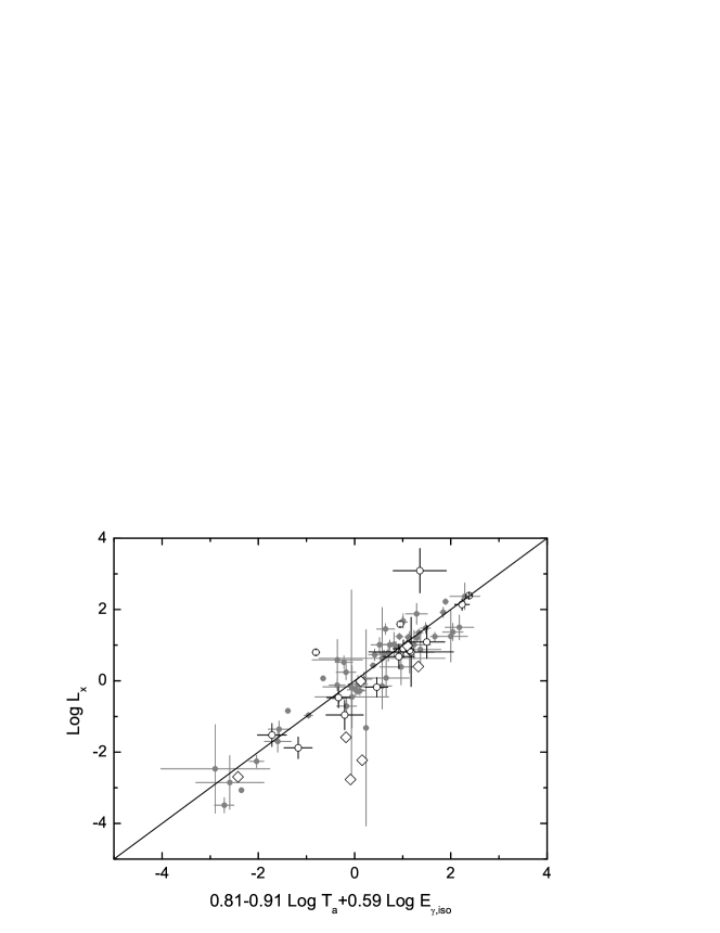
Figure 3: The best-fit correlation between $L_{\rm X}$, $T_{\rm a}$ and $E_{\gamma,\rm iso}$ for all the 77 GRBs of D2010. The units of all physical quantity are the same as Figure 2. The X-axis is a combined quantity of $0.81-0.91\log{T_{\rm a}}+0.59\log E_{\gamma,\rm iso}$. The filled points correspond to the observed data of 55 “golden” GRBs with error bars. The hollow diamonds correspond to 7 GRBs with too large error bars to be plotted in the figure, and the hollow circles correspond to other 15 discarded events. The solid line is the best fit for all the 77 data points.

In order to directly compare with the L-T correlation suggested by D2010, we have also fit the two-parameter correlation for our sample. The best-fit equation is

$$\begin{array}[]{rcl}{\rm log}(\frac{L_{\rm X}}{10^{47}\rm erg/s})=(0.78\pm 0.14)-(1.16\pm 0.16){\rm\leavevmode\nobreak\ log}(\frac{T_{\rm a}}{10^{3}\rm s}).\end{array}$$ (8)

This equation is consistent with the L-T correlation derived in D2010. Comparing Eq. (8) with Eq. (7) and from Figure 2, we find that the error bars of the constants in Eq. (8) (i.e. the L-T correlation) are generally significantly larger than those of Eq. (7) (i.e. the L-T-E correlation). Additionally, in the two-parameter fitting of Eq. (8), the intrinsic scatter is $0.85\pm 0.10$, which is also markedly larger than that in the three-parameter correlation case ($0.43\pm 0.05$). From the comparison, we see that the L-T-E correlation is really significantly tighter than the L-T correlation.

For our GRB sample, we additionally find that the correlation coefficient of our L-T-E statistics is $r=0.92$ and the chance probability is $P=1.05\times 10^{-20}$. On the contrary, the correlation coefficient of the L-T statistics of the same sample is $r=-0.73$ and the corresponding chance probability is $P=5.55\times 10^{-8}$. This also shows that the L-T-E correlation is much tighter than the L-T correlation.

4 Discussion and Conclusions

In this paper, a new three-parameter correlation is found for the GRBs with an obvious plateau phase in the afterglow. This L-T-E correlation is tighter than the L-T correlation reported in D2010. It has been shown that the intrinsic scattering of our L-T-E correlation is significantly smaller than that of the L-T correlation, and the correlation coefficient is correspondingly larger. However, we note that the intrinsic scatter of the L-T-E correlation is still larger than that of some correlations derived from prompt GRB emission (Guidorzi et al. 2006; Amati et al. 2008). In the future, more samples and more delicate selections might help to improve the result.

The plateau phase (or the shallow decay segment) is an interesting characteristics of many GRB afterglows (Zhang et al. 2006; Nousek et al. 2006). This phenomenon can be explained as continuous energy injection from the central engine after the prompt burst (Rees & Mészáros 1998; Dai & Lu 1998; Zhang & Mészáros 2001; Dai 2004; Kobayashi & Zhang 2007; Yu & Dai 2007; Xu et al. 2009; Yu et al. 2010; Dall^′Osso et al. 2011), or by the two component models (Corsi & Mészáros 2009), or by structured jets (Eichler & Granot 2006; Granot et al. 2006; Panaitescu 2007; Yamazaki 2009; Xu & Huang 2010), or even as due to dust scattering (Shao & Dai 2007; Shao et al. 2008). According to our L-T-E correlation (Eq. (7)), the X-ray luminosity at the end time of the plateau can be expressed as a function of the end time and the isotropic $\gamma$-ray energy release as,

$$L_{\rm X}\propto T_{\rm a}^{-0.87\pm 0.09}E_{\gamma,\rm iso}^{0.88\pm 0.08}.$$ (9)

We believe that this relation can give useful constraint on the underlying physics.

For the energy injection model, a natural mechanism is the dipole radiation from the spinning down of a magnetar at the center of the fireball. Note that the injected energy may not be Poynting flux, but can be electron-positron pairs (Dai 2004). These pairs interact with the fireball material, leading to the formation of a relativistic wind bubble. When the energy injection dominates the dynamical evolution of the external shock, the afterglow intensity should naturally be proportional to the energy injection power. So, $L_{\rm X}$ is actually a measure of the energy injection rate. According to Eq. (9), $L_{\rm X}$ is roughly inversely proportional to the timescale of the energy injection, $T_{\rm a}$. It hints that the energy reservoir should be roughly a constant. This is consistent with the energy injection model, which usually assumes that the central engine is a rapidly rotating millisecond magnetar. In different GRBs, the surface magnetic field intensities of the central magnetars may be quite different, leading to various energy injection luminosities and energy injection timescales. But the total energy available for energy injection is relatively constant (about rotational energy of the magnetar). It is mainly constrained by the limiting angular velocity of the magnetar, which again is determined by the equation of state of neutron stars. Additionally, according to Dai (2004), in order to produce an obvious plateau in the afterglow lightcurve, the total injected energy must be comparable to the original fireball energy (which may be comparable to $E_{\gamma,\rm iso}$). This requirement is again roughly consistent with the item of $E_{\gamma,\rm iso}^{0.88\pm 0.08}$ in Eq. (9). Based on the above analysises, we argued that the L-T-E correlation strongly supports the energy injection model of magnetars. It also indicates that the newly born millisecond magnetars associated with GRBs provide a good standard candle in our Universe. Thus the L-T-E correlation may potentially be used to test the cosmological models.

Our sample contains 47 long GRBs and 8 intermediate class GRBs. From Figure 1, we see that both of these two classes are consistent with the same L-T-E correlation. Howerer, note that they behave very differently in frame work of the two-parameter L-T correlation. This is another important advantage of our three-parameter correlation. It indicates that magnetars may also form in intermediate class GRBs, and their limiting spinning is just similar to those magnetars born in long GRBs. A natural problem will be raised as to whether short GRBs with plateau phase in the afterglow also obey the same correlation. Unfortunately, the number of short GRBs meeting the requirement is currently too few.

It is worth noting that many interesting physics could be involved in newly born magnetars (Dall^′Osso et al. 2009). The tops include the emission of gravitational waves, the cooling process, the evolution of the magnetic axis, etc. Some of the physics may affect the the energy injection process of the newly born magnetar delicately. We believe that further studies on the new three-parameter correlation may give useful constraints on the physics of newly born magnetars.

GRB	$z$	${\rm Log}[L_{\rm X}/(\rm erg/s)]$	${\rm Log}[T_{\rm a}/(\rm s)]$	${\rm Log}[E_{\gamma,\rm iso}/(\rm erg)]$	Type
050315	1.95	47.05 $\pm$ 0.19	3.92 $\pm$ 0.17	52.85 $\pm$ 0.012	Long
050319	3.24	47.52 $\pm$ 0.18	4.04 $\pm$ 0.17	52.90 $\pm$ 0.057	Long
050401	2.9	48.45 $\pm$ 0.15	3.28 $\pm$ 0.14	52.50 $\pm$ 0.098	Long
050416A	0.65	46.29 $\pm$ 0.23	2.97 $\pm$ 0.21	51.02 $\pm$ 0.027	Long
050505	4.27	48.03 $\pm$ 0.34	3.67 $\pm$ 0.33	53.26 $\pm$ 0.019	Long
050724	0.26	44.53 $\pm$ 1.24	4.92 $\pm$ 1.22	50.17 $\pm$ 0.055	IC
050730	3.97	48.68 $\pm$ 0.07	3.44 $\pm$ 0.04	53.26 $\pm$ 0.017	Long
050801	1.38	47.86 $\pm$ 0.17	2.17 $\pm$ 0.16	51.49 $\pm$ 0.066	Long
050802	1.71	47.43 $\pm$ 0.06	3.52 $\pm$ 0.06	52.59 $\pm$ 0.021	Long
050803	0.42	46.55 $\pm$ 0.87	2.74 $\pm$ 0.81	51.46 $\pm$ 0.069	Long
050814	5.3	47.88 $\pm$ 0.47	3.13 $\pm$ 0.45	53.29 $\pm$ 0.029	Long
050824	0.83	45.30 $\pm$ 0.29	4.65 $\pm$ 0.27	51.13 $\pm$ 0.052	Long
050922C	2.2	48.92 $\pm$ 0.07	2.08 $\pm$ 0.07	52.77 $\pm$ 0.009	Long
051016B	0.94	47.59 $\pm$ 0.57	3.22 $\pm$ 0.55	51.01 $\pm$ 0.034	Long
051109A	2.35	48.01 $\pm$ 0.13	3.4 $\pm$ 0.11	52.72 $\pm$ 0.018	Long
051109B	0.08	43.51 $\pm$ 0.21	3.64 $\pm$ 0.19	48.55 $\pm$ 0.064	Long
051221A	0.55	44.74 $\pm$ 0.16	4.51 $\pm$ 0.16	51.40 $\pm$ 0.014	IC
060108	2.03	46.50 $\pm$ 0.13	3.92 $\pm$ 0.13	51.94 $\pm$ 0.027	Long
060115	3.53	47.80 $\pm$ 0.57	3.09 $\pm$ 0.55	52.99 $\pm$ 0.023	Long
060116	6.6	49.37 $\pm$ 0.33	1.8 $\pm$ 0.3	53.33 $\pm$ 0.082	Long
060202	0.78	45.64 $\pm$ 0.23	4.74 $\pm$ 0.23	52.00 $\pm$ 0.040	Long
060206	4.05	48.65 $\pm$ 0.10	3.15 $\pm$ 0.1	52.79 $\pm$ 0.013	Long
060502A	1.51	47.27 $\pm$ 0.19	3.85 $\pm$ 0.21	52.59 $\pm$ 0.012	IC
060510B	4.9	47.39 $\pm$ 0.49	3.78 $\pm$ 0.48	53.64 $\pm$ 0.011	Long
060522	5.11	48.51 $\pm$ 0.33	2.07 $\pm$ 0.31	53.05 $\pm$ 0.026	Long
060604	2.68	47.24 $\pm$ 0.19	3.98 $\pm$ 0.18	52.21 $\pm$ 0.069	Long
060605	3.8	47.76 $\pm$ 0.09	3.48 $\pm$ 0.08	52.66 $\pm$ 0.034	Long
060607A	3.08	45.68 $\pm$ 2.75	4.14 $\pm$ 0.02	53.12 $\pm$ 0.012	Long
060614	0.13	43.93 $\pm$ 0.05	5.01 $\pm$ 0.05	51.32 $\pm$ 0.006	IC
060707	3.43	48.01 $\pm$ 0.40	2.94 $\pm$ 0.36	52.93 $\pm$ 0.025	Long
060714	2.71	48.22 $\pm$ 0.08	3.11 $\pm$ 0.07	53.06 $\pm$ 0.016	Long
060729	0.54	46.17 $\pm$ 0.04	4.73 $\pm$ 0.04	51.69 $\pm$ 0.021	Long
060814	0.84	46.69 $\pm$ 0.06	4.01 $\pm$ 0.06	52.97 $\pm$ 0.004	Long
060906	3.69	47.73 $\pm$ 0.13	3.62 $\pm$ 0.12	53.26 $\pm$ 0.042	Long
060908	2.43	48.24 $\pm$ 0.11	2.46 $\pm$ 0.09	53.03 $\pm$ 0.010	Long
060912A	0.94	46.37 $\pm$ 0.23	2.97 $\pm$ 0.18	51.91 $\pm$ 0.020	IC
061121	1.31	48.35 $\pm$ 0.10	3 $\pm$ 0.09	53.47 $\pm$ 0.004	Long
070110	2.35	48.25 $\pm$ 0.72	1.89 $\pm$ 0.37	52.90 $\pm$ 0.033	Long
070208	1.17	46.88 $\pm$ 0.15	3.63 $\pm$ 0.14	51.58 $\pm$ 0.060	Long
070306	1.49	47.07 $\pm$ 0.05	4.42 $\pm$ 0.04	53.18 $\pm$ 0.008	Long

Table 1: 55 GRBs of our sample. Data of the second, third, and forth columns are taken from D2010, the fifth column, $E_{\gamma,\rm iso}$, are calculated from Equation (2), where $S_{\rm bolo}$ are taken from Wang et al. (2011). The last column is the type of the GRB, where Long means long GRB and IC is intermediate class GRB. All the error bars are $1\sigma$ range.

GRB	$z$	${\rm Log}[L_{\rm X}/(\rm erg/s)]$	${\rm Log}[T_{\rm a}/(\rm s)]$	${\rm Log}[E_{\gamma,\rm iso}/(\rm erg)]$	Type
070506	2.31	47.63 $\pm$ 1.42	2.87 $\pm$ 1.42	51.82 $\pm$ 0.029	Long
070508	0.82	48.20 $\pm$ 0.02	2.75 $\pm$ 0.02	53.11 $\pm$ 0.004	Long
070529	2.5	48.40 $\pm$ 0.15	2.34 $\pm$ 0.15	53.04 $\pm$ 0.025	Long
070714B	0.92	46.85 $\pm$ 0.20	3.03 $\pm$ 0.19	52.30 $\pm$ 0.033	IC
070721B	3.63	47.08 $\pm$ 0.51	3.58 $\pm$ 0.51	53.34 $\pm$ 0.035	Long
070802	2.45	46.84 $\pm$ 2.72	3.68 $\pm$ 0.62	51.96 $\pm$ 0.047	Long
070809	0.22	44.15 $\pm$ 0.76	4.09 $\pm$ 0.75	49.43 $\pm$ 0.062	IC
070810A	2.17	47.97 $\pm$ 0.13	2.83 $\pm$ 0.12	52.26 $\pm$ 0.023	IC
071020	2.15	49.22 $\pm$ 0.05	1.84 $\pm$ 0.05	52.87 $\pm$ 0.016	Long
080310	2.42	46.72 $\pm$ 0.11	4.08 $\pm$ 0.11	52.88 $\pm$ 0.023	Long
080430	0.77	46.03 $\pm$ 0.08	4.29 $\pm$ 0.08	51.68 $\pm$ 0.022	Long
080603B	2.69	48.88 $\pm$ 0.26	2.92 $\pm$ 0.24	53.07 $\pm$ 0.011	Long
080810	3.35	48.24 $\pm$ 0.08	3.28 $\pm$ 0.07	53.42 $\pm$ 0.031	Long
081008	1.97	47.79 $\pm$ 0.24	2.95 $\pm$ 0.22	52.85 $\pm$ 0.047	Long
090423	8.26	48.48 $\pm$ 0.11	2.95 $\pm$ 0.1	53.03 $\pm$ 0.018	Long