An “algebraic” reconstruction of piecewise-smooth functions from integral measurements

Abstract.

This paper presents some results on a well-known problem in Algebraic Signal Sampling and in other areas of applied mathematics: reconstruction of piecewise-smooth functions from their integral measurements (like moments, Fourier coefficients, Radon transform, etc.). Our results concern reconstruction (from the moments or Fourier coefficients) of signals in two specific classes: linear combinations of shifts of a given function, and “piecewise $D$-finite functions” which satisfy on each continuity interval a linear differential equation with polynomial coefficients. In each case the problem is reduced to a solution of a certain type of non-linear algebraic system of equations (“Prony-type system”). We recall some known methods for explicitly solving such systems in one variable, and provide extensions to some multi-dimensional cases. Finally, we investigate the local stability of solving the Prony-type systems.

1. Introduction

It is well known that the error in the best approximation of a $C^{k}$-function $f$ by an $N$-th degree Fourier polynomial is of order ${C\over{N^{k}}}$. The same holds for algebraic polynomial approximation and for other basic approximation tools (see e.g. [21, Chapters IV, VI], and [32, Vol.I, Chapter 3, Theorem 13.6]). However, for $f$ with singularities, in particular, with discontinuities, the error is much larger: its order is ${C\over{\sqrt{N}}}$. Considering the so-called Kolmogorow $N$-width of families of signals with moving discontinuities one can show that any linear approximation method provides the same order of error, if we do not fix a priori the discontinuities’ position (see [11], Theorem 2.10). Another manifestation of the same problem is the “Gibbs effect” - a relatively strong oscillation of the approximating function near the discontinuities. Practically important signals usually do have discontinuities, so the above feature of linear representation methods presents a serious problem in signal reconstruction. In particular, it visibly appears near the edges of images compressed by JPEG, as well as in the noise and low resolution of the CT and MRI images.

Recent non-linear reconstruction methods, in particular, Compressed Sensing ([6, 7]) and Algebraic Sampling ([8, 19, 23, 10, 15]), address this problem in many cases. Both approaches appeal to an a priori information on the character of the signals to be reconstructed, assuming their “simplicity” in one or another sense. Compressed sensing assumes only a sparse representation in a certain (wavelets) basis, and thus it presents a rather general and “universal” approach. Algebraic Sampling usually requires more specific a priori assumptions on the structure of the signals, but it promises a better reconstruction accuracy. In fact, we believe that ultimately the Algebraic Sampling approach has a potential to reconstruct “simple signals with singularities” as good as smooth ones. The most difficult problem in this approach seems to be estimating the accuracy of solution of the nonlinear systems arising.

Our purpose in this paper is to further substantiate the Algebraic Sampling approach. On one hand, we present two algebraic reconstruction methods for generic classes of signals. The first one is reconstruction of combinations of shifts of a given function from the moments and Fourier coefficients (Section 2). The second one concerns piecewise $D$-finite moment inversion (Section 4). On the other hand, we consider some typical nonlinear systems arising in these reconstruction schemes. We describe the methods of their solution (Section 3), and provide some explicit bounds on their local stability (Section 5). We also present results of some numerical experiments in Section 6.

Our ultimate goal may be stated in terms of the following conjecture (which seems to be supported also by the results of [9, 18, 14, 30, 23]):

There is a non-linear algebraic procedure reconstructing any signal in a class of piecewise $C^{k}$-functions (of one or several variables) from its first $N$ Fourier coefficients, with the overall accuracy of order ${C\over{N^{k}}}$. This includes the discontinuities’ positions, as well as the smooth pieces over the continuity domains.

Recently [4] we have shown that at least half the conjectured accuracy can be achieved. However, the question of maximal possible accuracy remains open. Our results presented in this paper can be considered as an additional step in this direction.

2. Linear combinations of shifts of a given function

Reconstruction of this class of signals from sampling has been described in [8, 19]. We study a rather similar problem of reconstruction from the moments. Our method is based on the following approach: we construct convolution kernels dual to the monomials. Applying these kernels, we get a Prony-type system of equations on the shifts and amplitudes.

Let us restate a general reconstruction problem, as it appears in our specific setting. We want to reconstruct signals of the form

(1) $$F(x)=\sum_{j=1}^{N}a_{j}f(x-x^{j})$$

where $f$ is a known function of $x=(x_{1},\ldots,x_{d})\in{\mathbb{R}}^{d}$, while the number $N$ of the shifts and the form (1) of the signal are known a priori. The parameters $a_{j},\ x^{j}=(x^{j}_{1},\dots,x^{j}_{d}),\ j=1,\dots N$ are to be found from a finite number of “measurements”, i.e. of linear (usually integral) functionals like polynomial moments, Fourier moments, shifted kernels, evaluation over some grid etc.

In this paper we consider only linear combinations of shifts of one known function $f$. Reconstruction of shifts of several functions based on “decoupling” via sampling at zeroes of the Fourier transforms of the shifted functions is presented in [29].

In what follows $x=(x_{1},\dots,x_{d}),t=(t_{1},\ldots,t_{d})\in{\mathbb{R}}^{d}$,  $j$  is a scalar index, while $k=(k_{1},\dots,k_{d}),\ i=(i_{1},\dots,i_{d})$ and $n=(n_{1},\dots,n_{d})$ are multi-indices. Partial ordering of multi-indices is given by $k\leq k^{\prime}\Leftrightarrow k_{p}\leq k^{\prime}_{p},\ p=1,\dots,d.$

Assume that a multi-sequence of functions $\varphi=\{\varphi_{k}(t)\},\;t\in{\mathbb{R}}^{d},\;k\geq(0,\dots,0)$ is fixed. We consider the measurements $\mu_{k}(F)$ provided by

(2) $$\mu_{k}(F)=\int F(t)\varphi_{k}(t)\operatorname{d}t,\ k\geq(0,\dots,0).$$

Our approach now works as follows: given $f$ and $\varphi=\{\varphi_{k}(t)\}$ we now try to find an “$f$-convolution dual” system of functions $\psi=\psi_{k}(t)$ in a form of certain “triangular” linear combinations

(3) $$\psi_{k}(t)=\sum_{0\leq i\leq k}C_{i,k}\varphi_{i}(t),\ k\geq(0,\dots,0).$$

More accurately, we try to find the coefficients $C_{i,k}$ in (3) in such a way that

(4) $$\int f(t-x)\psi_{k}(t)\operatorname{d}t=\varphi_{k}(x).$$

We shall call a sequence $\psi=\{\psi_{k}(t)\}$ satisfying (3),  (4)  $f$ - convolution dual to $\varphi$. Below we shall find explicitly convolution dual systems to the usual and exponential monomials.

We consider a general problem of finding convolution dual sequences to a given sequence of measurements as an important step in the reconstruction problem. Notice that it can be generalized by dropping the requirement of a specific representation (3): $\psi_{k}(t)=\sum_{i=0}^{k}C_{i,k}\varphi_{i}(t)$. Instead we can require only that $\int f(t)\psi_{k}(t)\operatorname{d}t$ be expressible in terms of the measurements sequence $\mu_{k}$. Also $\varphi_{k}$ in (4) can be replaced by another a priori chosen sequence $\eta_{k}$. This problem leads, in particular, to certain functional equations, satisfied by polynomials and exponential functions, as well as exponential polynomials and some kinds of elliptic functions (see [28]).

Now we have the following result:

Theorem 1.

Let a sequence $\psi=\psi_{k}(t)$ be $f$-convolution dual to $\varphi$. Define $M_{k}$ by $M_{k}=\sum_{0\leq i\leq k}C_{i,k}\mu_{i}.$ Then the parameters $a_{j}$ and $x^{j}$ in (1) satisfy the following system of equations (“generalized Prony system”):

(5) $$\sum_{j=1}^{N}a_{j}\varphi_{k}(x^{j})=M_{k},\ \ k\geq(0,\dots,0).$$

Proof.

By definition of $M_{k}$ and via (3) and (4) we have for each $k\geq(0,\dots,0)$

$$M_{k}=\sum_{0\leq i\leq k}C_{i,k}\mu_{i}=\int F(t)\sum_{0\leq i\leq k}C_{i,k}\varphi_{i}(t)\operatorname{d}t=$$

$$=\int F(t)\psi_{k}(t)\operatorname{d}t=\sum_{j=1}^{N}a_{j}\int f(t-x^{j})\psi_{k}(t)\operatorname{d}t=\sum_{j=1}^{N}a_{j}\varphi_{k}(x^{j}).$$

This completes the proof. ∎

According to Theorem 1, in order to reduce the reconstruction problem with the measurements (2) and for signals of the a priori known form (1) to a solution of the generalized Prony system we have to find an $f$ - convolution dual system $\psi=\psi_{k}(t)$ to the measurements kernels $\varphi$. In fact we need only the coefficients $C_{i,k}$. Having these coefficients, we compute $M_{k}$ and get system (5).

Solvability of system (5) and robustness of its solution depend on the measurements kernels $\varphi$. Specific examples are considered below.

2.1. Reconstruction from moments

We are given a finite number of moments of a signal $F(x)=\sum_{j=1}^{N}a_{j}f(x-x^{j})$ as in (1) in the form

(6) $$m_{k}=\int F(t)t^{k}\operatorname{d}t,\ k=(k_{1},\dots,k_{d})\geq(0,\dots,0).$$

So here $\varphi_{k}(x)=x^{k_{1}}_{1}\cdots x^{k_{d}}_{d}$ for each multi-index $k$. We look for the dual functions $\psi_{k}$ satisfying the convolution equation

(7) $$\int f(t-x)\psi_{k}(t)\operatorname{d}t=x^{k}$$

for each multi-index $k$. To solve this equation we apply Fourier transform to both sides of (7). Assuming that $\hat{f}(0)\neq 0$ and that $\hat{f}(\omega)$ has the derivatives of all the orders at $0$ we find (see [28]) that there is a unique solution to (7) provided by

(8) $$\varphi_{k}(x)=\sum_{l\leq k}C_{k,l}x^{l},$$

where

$$C_{k,l}=\frac{1}{(\sqrt{2\pi})^{d}}{k\choose l}(-i)^{k+l}\left[\left.\frac{\partial^{k-l}}{\partial\omega^{k-l}}\right|_{\omega=0}\frac{1}{\hat{f}(\omega)}\right].$$

The assumption $\hat{f}(0)\neq 0$ is essential in the construction of the $f$-convolution dual system for the monomials as well as for other measurement kernels (as well as in the study of the shifts of a given function in general). The above calculation can be applied, with proper modifications, in more general situations (see [28]). On the other hand, the assumption of differentiability of $\hat{f}$ at zero is not very restrictive, in particular, if we work with signals with finite support.

Returning to the moments reconstruction, we set the generalized polynomial moments $M_{k}$ as

(9) $$M_{k}=\sum_{l\leq k}C_{k,l}m_{l}$$

and obtain, as in Theorem 1, the following system of equations:

(10) $$\sum^{N}_{j=1}a_{j}(x^{j})^{k}=\sum^{N}_{j=1}a_{j}(x^{j}_{1})^{k_{1}}\cdots(x^{j}_{d})^{k_{d}}=M_{k},\ k\geq(0,\dots,0).$$

This system is called “multidimensional Prony system”. It appears in numerous problems of theoretical and applied mathematics. In Section 3 below we recall one of the classical methods for its solution in one-dimensional case, and describe, under certain assumptions, a method for its solution in several dimensions. Local stability of the solutions of the one-dimensional Prony system is discussed in Section 5.

2.2. Fourier case

The signal has the same form as in section 2.1: $F(x)=\sum_{j=1}^{N}a_{j}f(x-x^{j})$. The measurement kernels $\varphi$ we now choose as the harmonics $\varphi_{k}(x)=e^{ikx}$. So our measurements are the Fourier coefficients $c_{k}(F)=\hat{f}(k)=\int F(x)e^{ikx}\operatorname{d}x.$

Let us assume now that $f$ satisfies the condition $\hat{f}(k)\neq 0$ for all integer $k$. Then the Fourier harmonics turn out to form essentially $f$-self-dual system: indeed, taking $\psi_{k}(x)=\frac{1}{\hat{f}(k)}e^{ikx}$ we get immediately that $\int f(t-x)\psi_{k}(t)\operatorname{d}t=\int f(t-x)\frac{1}{\hat{f}(k)}e^{ikt}\operatorname{d}t=\frac{\hat{f}(k)}{\hat{f}(k)}e^{ikx}=\varphi_{k}(x).$

According to our general scheme we put now $M_{k}=\frac{1}{\hat{f}(k)}c_{k}(F)$ and get a system of the form

(11) $$\frac{1}{\hat{f}(k)}c_{k}(F)=M_{k}=\sum^{N}_{j=1}a_{j}e^{ikx^{j}}=\sum^{N}_{j=1}a_{j}(\rho^{j})^{k},\ k\geq(0,\dots,0),$$

where $\rho^{j}=e^{ix^{j}}$. This is once more a multidimensional Prony system as in (10), with the nodes on the complex unit circle.

2.3. Further extensions

The approach above can be extended in the following directions:

1. Reconstruction of signals built from several functions or with the addition of dilations also can be investigated (a perturbation approach where the dilations are approximately 1 is studied in [26]).

2. Further study of “convolution duality” in [26] provides a certain extension of the class of signals and measurements allowing for a closed - form reconstruction.

3. Prony system

3.1. One-dimensional case

Let us start with the classical case of one-dimensional Prony system:

(12) $$\sum^{N}_{j=1}a_{j}(x^{j})^{k}=m_{k},\ x^{j}\in{\mathbb{R}},\ k=0,1,\dots.$$

This system appears in many branches of mathematics (see [20]). There are several solution methods available, for instance direct nonlinear minimization (see e.g. [9]), the polynomial realization (original Prony method, [24]) or the state-space approach ([25]). Let us give a sketch of a method based on Padé approximation techniques which is rather close to the original Prony method. To simplify the presentation we shall assume that we know a priori that all the nodes $x^{j}$ are pairwise distinct. General case is treated similarly ([22], see also [31]).

Consider a “moments generating function” $I(z)=\sum_{k=0}^{\infty}m_{k}z^{k},\ z\in{\mathbb{C}}.$ Assuming the equations (12) are satisfied for all $k=0,1,\dots$ and summing up the geometric progressions we get

(13) $$I(z)=\sum_{j=1}^{N}{a_{j}\over{1-x^{j}z}}.$$

So $I(z)$ is a rational function of degree $N$ tending to zero as $z\rightarrow\infty$. The unknowns $a_{j}$ and ${1\over{x^{j}}}$ in (12) are the poles and the residues of $I(z)$, respectively.

Now in order to find $I(z)$ explicitly from the first $2N$ moments $m_{0},m_{1},\dots,m_{2N}$ we use the Padé approximation approach (see [22]): write $I(z)$ as ${{P(z)}\over{Q(z)}}$ with polynomials $P(z)=A_{0}+A_{1}z+\dots+A_{N-1}z^{N-1}$ and $Q(z)=B_{0}+B_{1}z+\dots+B_{N}z^{N}$ of degrees $N-1$ and $N$, respectively.

Multiplying by $Q$ we have $I(z)Q(z)=P(z)$. Now equating the coefficients on both sides we get the following system of linear equations:

$m_{0}B_{0}=A_{0}$

$m_{0}B_{1}+m_{1}B_{0}=A_{1}$

………………………..

$m_{0}B_{N-1}+m_{1}B_{N-2}+\dots+m_{N-1}B_{0}=A_{N-1}$

$m_{0}B_{N}+m_{1}B_{N-1}+\dots+m_{N-1}B_{1}+m_{N}B_{0}=0$

$m_{1}B_{N}+m_{2}B_{N-1}+\dots+m_{N}B_{1}+m_{N+1}B_{0}=0$

…………………………

The rest of the equations in this system are obtained by further shifts of the indices of the moments, and so they form a Hankel-type matrix.

Now, being a rational function of degree $N$, $I(z)$ is uniquely defined by its first $2N$ Taylor coefficients (the difference of two such functions cannot vanish at zero with the order higher than $2N-1$). We conclude that the linear system consisting of the first $2N$ equations as above is uniquely solvable up to a common scaling of $P$ and $Q$ (of course, this fact follows also form a general Padé approximation theory - see [22]).

Now a solution procedure for the Prony system can be described as follows:

1. Solve a linear system of the first $2N$ equations as above (with the coefficients - the known moments $m_{k}$) to find the moments generating function $I(t)$ in the form $I(z)={{P(z)}\over{Q(z)}}$.

2. Represent $I(z)$ in a standard way as the sum of elementary fractions $I(z)=\sum_{j=1}^{N}{a_{j}\over{1-x^{j}z}}$. (Equivalently, find poles and residues of $I(z)$). Besides algebraic operations, this requires just finding the roots of the polynomial $Q(z)$. Then $(a_{j},x^{j}),\ j=1,\dots,N$ form the unique solution of the Prony system (12).

3.2. Multi-dimensional case

Let us recall our multi-dimensional notations: $x=(x_{1},\dots,x_{d})\in{\mathbb{R}}^{d}$,  $j$  is a scalar index, while $k=(k_{1},\dots,k_{d}),\ i=(i_{1},\dots,i_{d})$ and $n=(n_{1},\dots,n_{d})$ are multi-indices. Partial ordering of multi-indices is given by $k\leq k^{\prime}\Leftrightarrow k_{p}\leq k^{\prime}_{p},\ p=1,\dots,d.$

Let $x^{j}=(x^{j}_{1},\dots,x^{j}_{d}),\ j=1,\dots,N.$ With the above notation, the multidimensional Prony system has exactly the same form as in the one-dimensional case:

(14) $$\sum^{N}_{j=1}a_{j}(x^{j})^{k}=m_{k},\ x^{j}\in{\mathbb{R}}^{d},\ k\geq(0,\dots,0).$$

Exactly as above we get that for $z=(z_{1},\dots,z_{d})\in{\mathbb{C}}^{d}$ the moments generating function $I(z)=\sum_{k\in{\mathbb{N}}^{d}}m_{k}z^{k}$ is a rational function of degree $Nd$ of the form

(15) $$I(z)=\sum_{j=1}^{N}a_{j}\prod_{l=1}^{d}\frac{1}{1-x^{j}_{l}z_{l}}\ .$$

Representing $I(z)$ as ${{P(z)}\over{Q(z)}}$ we get exactly in the same way as above an infinite system of linear equations for the coefficients of $P$ and $Q$, with a Hankel-type matrix formed by the moments $m_{k}$. By the same consideration as above, after we take enough equations in this system the solution is unique up to a rescaling (see [1, 22] and references therein).

However, from this point the multi-dimensional situation becomes essentially more complicated. While in dimension one $I(z)$ can be, essentially, any rational function of degree $N$ (naturally represented as the sum of elementary fractions), in several variables $I(z)$ has a very special form given by (15). This fact can be easily understood via counting the degrees of freedom: the number of unknowns in (14) is $N(d+1)$ while a rational function of degree $Nd$ in $d$ variables has much more coefficients than that, for $d>1$. It would be desirable to use as many equations from (14) as the number of unknowns, but the method outlined above ignores a specific structure of $I(z)$ and requires as many equations as in a Padé reconstruction for a general rational function of degree $Nd$.

We treat this problem in [28] analyzing the structure of singularities of $I(z)$ and on this base proposing a robust reconstruction algorithm. Let us give here one simple special case of this algorithm, which separates the variables in the problem.

3.2.1. Separation of variables in the multi-dimensional Prony system

Let us assume that we know a priori that the solution $(a_{j},x^{j}),\ j=1,\dots,N$ of multi-dimensional Prony system (14) is such that all the coordinates $x^{j}_{l},\ l=1,\dots,d$ of the points $x^{j},\ j=1,\dots N$ are pairwise distinct. Moreover, we assume that $a_{j_{1}}\neq a_{j_{2}}$ for $j_{1}\neq j_{2}$. Under these assumptions we proceed as follows:

Consider “partial moment generating functions” $I_{m}(t),\ t\in{\mathbb{C}},\ m=1,\dots,d$, defined by

(16) $$I_{m}(t)=\sum_{r=1}^{\infty}m_{re_{m}}t^{r},$$

where $e_{m}$ is a multi-index with $(e_{m})_{j}=0$ for $m\neq j$ and $1$ otherwise. We have the following simple fact:

Proposition 2.

$I_{m}(t)$ is a one-dimensional moments generating function of the form

(17) $$I_{m}(t)=\sum_{j=1}^{N}a_{j}\frac{1}{1-x^{j}_{m}t}.$$

It coincides with the restriction of $I(z)$ to the $m$-th coordinate axis in ${\mathbb{C}}^{d}$.

Proof.

Let us evaluate $I(z)$ along the $m$-th coordinate axis, that is on the line $z=te_{m}$ with $e_{m}$ as above and $t\in{\mathbb{C}}$. We get

$$I(te_{m})=\sum_{j=1}^{N}a_{j}\prod_{l=1}^{d}\frac{1}{1-x^{j}_{l}t({e_{m}})_{l}}=\sum_{j=1}^{N}a_{j}\frac{1}{1-x^{j}_{m}t}$$

which is the moments generating function (17). Now, to express $I_{m}(t)$ through the multi-dimensional moments $m_{k}$ we notice that any monomial $x^{k}$, with $k\neq pe_{m}$ vanishes identically on the $m$-th coordinate axis. Hence

$$I(te_{m})=\sum_{r=0}^{\infty}m_{re_{m}}t^{r}.$$

This shows that $I_{m}(t)\equiv I(te_{m})$ and completes the proof of the proposition. ∎

Now applying the method described in Section (3.1) above we find for each $m=1,\dots,d$ the coordinates $x^{1}_{m},\dots,x^{N}_{m}$ and (repeatedly) the coefficients $a_{1},\dots,a_{N}$. It remains to arrange these coordinates into the points $x^{j}=(x^{j}_{1},\dots,x^{j}_{d})$. This presents a certain combinatorial problem, since Prony system (14) is invariant under permutations of the index $j$. Under the assumptions above we proceed as follows: for each $m=1,\dots,d$ we have obtained the (unordered) collection of the pairs $(a_{j},x^{j}_{m}),\ j=1,\dots,N$. By assumptions $a_{j_{1}}\neq a_{j_{2}}$ for $j_{1}\neq j_{2}$. Hence we can arrange in a unique way all the pairs $(a_{j},x^{j}_{m}),\ j=1,\dots,N,\ m=1,\dots,d$ into the string $[(a_{1},x^{1}_{1}),\dots,(a_{1},x^{1}_{d})],\dots,[(a_{N},x^{N}_{1}),\dots,(a_{N},x^{N}_{d})].$ This gives us the desired solution of multi-dimensional Prony system (14).

Notice that the assumption $a_{j_{1}}\neq a_{j_{2}}$ for $j_{1}\neq j_{2}$ is essential here. Indeed, for $x_{1}\neq x_{2}$ and $x^{1}=(x_{1},x_{2}),\ x^{2}=(x_{2},x_{1}),\ \hat{x}^{1}=(x_{1},x_{1}),\ \hat{x}^{2}=(x_{2},x_{2})$ we have $m_{k}=(x^{1})^{k}+(x^{2})^{k}\equiv(\hat{x}^{1})^{k}+(\hat{x}^{2})^{k}$ for $k$ on each of the coordinate axes. So the (unique up to permutations of the index $j$) solution of the Prony system cannot be reconstructed from these moments only.

Another remark is that the separation of variables as described above requires knowledge of $2dN$ moments $m_{k}$ ($2N$ on each of the coordinate axes). This is almost twice more than $N(d+1)$ unknowns. This number can be significantly reduced in some cases. See [28] for further investigation in both of these directions.

Stability estimates for the solution of one-dimensional Prony system (Section 5) can be easily extended to the case considered in the present subsection. We do not give here explicit statement of this result.

4. Reconstruction of piecewise $D$-finite functions from moments

In this section we present an overview of our previous findings on algebraic reconstruction of a certain general class of signals. See [3] for the complete details.

Let $g:[a,b]\to\mathbb{R}$ consist of $N+1$ “pieces” $g_{0},\dotsc g_{N}$ with $N\geq 0$ jump points

$$a=x_{0}<x_{1}\dotsc<x_{N}<x_{N+1}=b$$

Furthermore, let $g$ satisfy on each continuity interval some linear homogeneous differential equation with polynomial coefficients: $\operatorname{\mathfrak{D}}g_{n}\equiv 0,\;n=0,\dotsc,N$ where

(18) $$\mathfrak{D}=\sum_{j=0}^{r}\biggl{(}\sum_{i=0}^{k_{j}}b_{i,j}x^{i}\biggr{)}\frac{\operatorname{d}^{j}}{\operatorname{d}x^{j}}\quad(b_{ij}\in\mathbb{R})$$

Each $g_{n}$ may be therefore written as a linear combination of functions $\{u_{i}\}_{i=1}^{r}$ which are a basis for the space $\mathcal{N}_{\operatorname{\mathfrak{D}}}=\{f:\operatorname{\mathfrak{D}}f\equiv 0\}$:

(19) $$g_{n}(x)=\sum_{i=1}^{r}\alpha_{i,n}u_{i}(x),\quad n=0,1,\dotsc,N$$

We term such functions $g$ “piecewise $D$-finite”. Many “simple” functions may be represented in this framework, such as polynomials, trigonometric polynomials and algebraic functions.

The sequence $\{m_{k}=m_{k}(g)\}$ is given by the usual moments

$$m_{k}(g)=\int_{a}^{b}x^{k}g(x)\operatorname{d}x$$

Piecewise $D$-finite Reconstruction Problem.

Given $r,\{k_{i}\},N,a,b$ and the moment sequence $\{m_{k}\}$ of a piecewise $D$-finite function $g$, reconstruct all the parameters $\{b_{i,j}\},\{x_{i}\},\{\alpha_{i,n}\}$.

The above problem can be solved as follows.

1. It turns out that the moment sequence of every piecewise $D$-finite function $g$ satisfies a linear recurrence relation, such that the coefficients of $\operatorname{\mathfrak{D}}$ annihilating every piece of $g$ and the discontinuity locations $\{x_{j}\}$ can be recovered from the moments by solving a linear systems of equations plus a nonlinear step of polynomial roots finding. As we shall explain below, in many cases this step is equivalent to solving a certain generalized form of the previously mentioned Prony system (12).

2. The function $g$ itself can be subsequently reconstructed by numerically calculating the basis for the space $\mathcal{N}_{\operatorname{\mathfrak{D}}}$ and solving an additional linear system of equations to recover the coefficients $\alpha_{i,n}$.

The above algorithm has been tested on reconstruction of piecewise polynomials, piecewise sinusoids and rational functions - see [3] for details. The results reported there were relatively accurate for low noise levels. In this paper we continue to explore the numerical stability of the method - see Sections 5 and 6.

Now let us show how the Prony system arises in the piecewise $D$-finite reconstruction method. Consider the distribution $\operatorname{\mathfrak{D}}g$. It is of the form (see [3, Theorem 2.12])

(20) $$\operatorname{\mathfrak{D}}g=\sum_{j=1}^{N}\sum_{i=0}^{l_{j}-1}a_{i,j}\delta^{(i)}\left(x-x_{j}\right)$$

where $x_{j}\in\mathbb{R}$ are the discontinuity locations, $a_{i,j}\in\mathbb{R}$ are the associated “jump magnitudes” which depend on the values $\{g^{(i)}(x_{j}^{\pm})\}$, and $\delta(x)$ is the Dirac $\delta$-function. In particular, when $g$ is just a piecewise constant function, we have $\operatorname{\mathfrak{D}}={\operatorname{d}\over\operatorname{d}x}$ and so

(21) $$\operatorname{\mathfrak{D}}g=\sum_{j=1}^{N}a_{j}\delta(x-x_{j})$$

where $a_{j}=g(x_{j}^{+})-g(x_{j}^{-})$. Let us now apply the moment transform to the equations (21) and (20). We get, correspondingly,

(22) $$m_{k}\left(\operatorname{\mathfrak{D}}g\right) = \sum_{j=1}^{N}a_{j}x_{j}^{k};$$

(23) $$m_{k}\left(\operatorname{\mathfrak{D}}g\right) = \sum_{j=1}^{N}\sum_{i=0}^{l_{j}-1}a_{i,j}k(k-1)\times\dots\times(k-i+1)x_{j}^{k-i}.$$

The system (22) is of course identical to the previously considered (12). However, the following question arises: how are the numbers in the left-hand side of (22) and (23) related to the known quantities $m_{k}\left(g\right)$? It turns out that the numbers $m_{k}\left(\operatorname{\mathfrak{D}}g\right)$ are certain linear combinations of these known moments, with coefficients which are determined by $\operatorname{\mathfrak{D}}$ in a well-defined way. The conclusion is as follows: if the operator $\operatorname{\mathfrak{D}}$ which annihilates every piece of $g$ is known (but the other parameters are not), then one can recover the discontinuity locations of $g$ by solving the Prony-like system (23). We term the system (23) “confluent Prony system”. It can be solved in a similar manner to the standard Prony system. A unique solution exists whenever all the $x_{j}$’s are distinct and the highest coefficients $a_{l_{j}-1,j}$ are nonzero. We provide the details in [2].

5. Accuracy of solving Prony-like systems

In the preceding sections we have shown that several algebraic methods for nonlinear reconstruction can be reduced to solving certain types of systems of equations, the most basic one of which is the Prony system (12), (22). A crucial factor for the eventual applicability of the reconstruction methods is the sensitivity of solving these systems to measurement errors.

In this section we consider two such systems - (22) and (23) and provide some theoretical results regarding the local sensitivity of their solution to noise. These results will hopefully enable further “global” analysis.

We consider the following question: if the measurements in the left-hand side of (22) are known with error at most $\varepsilon$, how well can one recover the unknowns $\{a_{j},x_{j}\}$? We regard this stability problem to be absolutely central in Algebraic Sampling. To our best knowledge, no general treatment of this problem exists, therefore we consider our results below to be a step in this direction.

For simplicity, let us assume that the number of equations in (22) equals the number of unknowns, which in this case is $P=2N$. Let us further consider the “measurement map” $\mathcal{P}:\mathbb{R}^{P}\to\mathbb{R}^{P}$ given by (22) (we call it the “Prony map”):

$$\mathcal{P}\bigl{(}\{a_{j}\},\{x_{j}\}\bigr{)}\stackrel{{\scriptstyle\text{def}}}{{=}}\{m_{k}\}_{k=0}^{P-1}$$

Then, one possible answer (by no means a complete one) to the question posed above can be given in terms of the local Lipschitz constant of the “solution map” $\mathcal{P}^{-1}$, whenever this inverse is defined. We then obtain the following result.

Theorem 3.

Let $\{m_{k}\}_{k=0,\dots,P-1}$ be the exact unperturbed moments of the model (21). Assume that all the $x_{j}$’s are distinct and also $a_{j}\neq 0$ for $j=1,\dots,N$. Now let $\widetilde{m_{k}}$ be perturbations of the above moments such that $\max_{k}|m_{k}-\widetilde{m_{k}}|<\varepsilon$. Then, for sufficiently small $\varepsilon$, the perturbed Prony system has a unique solution which satisfies:

$$|\widetilde{x}_{j}-x_{j}| \leq C_{1}\varepsilon|a_{j}|^{-1}$$

$$|\widetilde{a}_{j}-a_{j}| \leq C_{1}\varepsilon$$

where $C_{1}$ is an explicit constant depending only on the geometry of $x_{1},\dotsc,x_{N}$.

Proof.

Consider the Jacobian determinant of the map $\mathcal{P}$. It is easily factorized as follows:

$$\operatorname{d}\mathcal{P}=\underbrace{\begin{bmatrix}1&0&\dots&1&0\\ x_{1}&1&\dots&x_{N}&1\\ \vdots\\ x_{1}^{P}&Px_{1}^{P-1}&\dots&x_{N}^{P}&Px_{N}^{P-1}\end{bmatrix}}_{\stackrel{{\scriptstyle\text{def}}}{{=}}V\left(x_{1},\dots,x_{N}\right)}\times\operatorname{diag}\{D_{1},\dots,D_{N}\}$$

where $D_{j}$ is a $2\times 2$ block

$$D_{j}\stackrel{{\scriptstyle\text{def}}}{{=}}\begin{bmatrix}1&0\\ 0&a_{j}\end{bmatrix}$$

The matrix $V=V\left(x_{1},\dots,x_{N}\right)$ is a special case of the so-called confluent Vandermonde matrix, well-known in numerical analysis ([5, 12, 13, 16]). In particular, the paper [12, Theorem 3] contains the following estimate for the norm of $V^{-1}$:

$$\|V^{-1}\|_{\infty}\leq\max_{1\leq i\leq N}b_{i}\prod_{j=1,j\neq i}^{N}\biggl{(}\frac{1+|x_{j}|}{|x_{i}-x_{j}|}\biggr{)}^{2}$$

where

$$b_{i}\stackrel{{\scriptstyle\text{def}}}{{=}}\max\biggr{(}1+|x_{i}|,1+2(1+|x_{i}|)\sum_{j\neq i}\frac{1}{|x_{j}-x_{i}|}\biggl{)}$$

Now since the $x_{j}$’s are distinct and $a_{j}\neq 0$, the Jacobian is non-singular and so in a sufficiently small neighbourhood of the exact solution, the map $\mathcal{P}$ is approximately linear. By the inverse function theorem

$$\operatorname{d}\mathcal{P}^{-1}=\operatorname{diag}\{D_{1}^{-1},\dots,D_{N}^{-1}\}\times V^{-1}$$

and so taking $C_{1}\stackrel{{\scriptstyle\text{def}}}{{=}}\|V^{-1}\|_{\infty}$ completes the proof. ∎

By a similar technique with slightly more involved calculations we obtain the following result for the system (23).

Theorem 4.

Let $\{m_{k}\}_{k=0,\dots,P-1}$ be the exact unperturbed moments of the model (20), where $P=\sum_{j=1}^{N}l_{j}+N$. Assume that all the $x_{j}$’s are distinct and also $a_{l_{j}-1,j}\neq 0$ for $j=1,\dots,N$. Now let $\widetilde{m_{k}}$ be perturbations of the above moments such that $\max_{k}|m_{k}-\widetilde{m_{k}}|<\varepsilon$. Then, for sufficiently small $\varepsilon$, the perturbed confluent Prony system has a unique solution which satisfies:

$$|\widetilde{a}_{i,j}-a_{i,j}| \leq\begin{cases}C_{2}\varepsilon&i=0\\ C_{2}\varepsilon\biggl{(}1+\frac{|a_{i-1,j}|}{|a_{l_{j}-1,j}|}\biggr{)}&1\leq i\leq l_{j}-1\end{cases}$$

$$|\widetilde{x}_{j}-x_{j}| \leq C_{2}\varepsilon\frac{1}{|a_{l_{j}-1,j}|}$$

where $C_{2}$ is a constant depending only on the nodes $x_{1},\dotsc,x_{N}$ and the multiplicities $l_{1},\dotsc,l_{N}$.

Proof outline.

As before, we obtain a factorization of the Jacobian determinant $\operatorname{d}\mathcal{P}$ as a product of a confluent Vandermonde matrix $V(x_{1},l_{1},\dots,x_{N},l_{N})$ (defined in a similar manner but with each column having $l_{j}-2$ “confluencies”) and the block diagonal matrix $D=\operatorname{diag}\{D_{1},\dots,D_{N}\}$ where

$$D_{j}=\begin{bmatrix}1&0&\cdots&0\\ 0&1&\cdots&a_{0,j}\\ \vdots&\vdots&\ \ddots&\vdots\\ 0&0&\cdots&a_{l_{j}-1,j}\end{bmatrix}$$

Inverting this expression and taking $C_{2}=\|V^{-1}\|_{\infty}$ completes the proof. ∎

An important generalization would be to consider the mappings

$$\mathcal{P}_{s}:\bigl{(}\{a_{i,j}\},\{x_{j}\}\bigr{)}\stackrel{{\scriptstyle\text{def}}}{{=}}\{m_{k}\}_{k=s}^{P+s-1}$$

and investigate the reconstruction error as $s\to\infty$. Such a formulation makes sense in the Fourier reconstruction problem ([4, 9, 11]). This is a work in progress and we plan to present the results separately ([2]).

6. Numerical experiments

We have tested the piecewise $D$-finite reconstruction method on a simple case of a piecewise-constant signal. The implementation details are identical to those used in [3, Appendix]. As can be seen from Figure 1, the reconstruction is accurate even in the presence of medium-level noise.

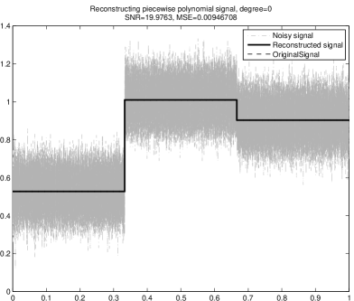
Figure 1. Reconstructing a piecewise-constant signal with two jumps. The reconstructed and the original are very close.

We have already mentioned that for a piecewise constant function $f$, the distribution $f^{\prime}$ is of the form (21). Therefore, the piecewise $D$-finite reconstruction problem for $f$ essentially reduces to solving the Prony system (22), and so the local estimates of Theorem 3 should apply in the case of a very small noise level. This prediction is partially confirmed by the results of our second experiment, presented in Figure 2. In particular, it can be seen that indeed $|\Delta x_{j}|\sim|a_{j}|^{-1}$, while the accuracy of other jump points $|\Delta x_{i}|$ does not depend on $|a_{j}|$ for $j\neq i$. While this is certainly an encouraging result, more investigation is clearly needed in order to fully understand the dependence of the error on all the parameters of the problem. Such an investigation should, in our opinion, concentrate on the global structure of the mapping $\mathcal{P}$.

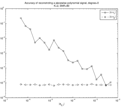
Figure 2. Dependence of the reconstruction accuracy on the magnitude of the jump.

References

- [1] G. A. Baker, P. Graves-Morris, Padé Approximants. Cambridge U.P., 1996.
- [2] D.Batenkov, Y.Yomdin, Accuracy of nonlinear reconstruction for discontinuous models, in preparation.
- [3] D.Batenkov, Moment inversion problem for piecewise -finite functions, Inverse Problems, 25(10):105001, October 2009.
- [4] Batenkov, D., Yomdin, Y. Algebraic Fourier reconstruction of piecewise smooth functions, to appear in Mathematics of Computation.
- [5] Å. Björck and T. Elfving. Algorithms for confluent Vandermonde systems. Numerische Mathematik, 21(2):130–137, 1973.
- [6] E. J. Candes̀. Compressive sampling. Proceedings of the International Congress of Mathematicians, Madrid, Spain, 2006. Vol. III, 1433–1452, Eur. Math. Soc., Zurich, 2006.
- [7] D. Donoho, Compressed sensing. IEEE Trans. Inform. Theory 52 (2006), no. 4, 1289–1306.
- [8] P.L. Dragotti, M. Vetterli and T. Blu, Sampling Moments and Reconstructing Signals of Finite Rate of Innovation: Shannon Meets Strang-Fix, IEEE Transactions on Signal Processing, Vol. 55, Nr. 5, Part 1, pp. 1741-1757, 2007.
- [9] K. Eckhoff, Accurate reconstructions of functions of finite regularity from truncated Fourier series expansions, Math. Comp. 64 (1995), no. 210, 671–690.
- [10] M. Elad, P. Milanfar, G. H. Golub, Shape from moments—an estimation theory perspective, IEEE Trans. Signal Process. 52 (2004), no. 7, 1814–1829.
- [11] B. Ettinger, N. Sarig. Y. Yomdin, Linear versus non-linear acqusition of step-functions, J. of Geom. Analysis, 18 (2008), 2, 369-399.
- [12] W. Gautschi. On inverses of Vandermonde and confluent Vandermonde matrices. Numerische Mathematik, 4(1):117–123, 1962.
- [13] W. Gautschi. On inverses of Vandermonde and confluent Vandermonde matrices III. Numerische Mathematik, 29(4):445–450, 1978.
- [14] A. Gelb, E. Tadmor, Detection of edges in spectral data II. Nonlinear enhancement, SIAM J. Numer. Anal. 38 (2000), 1389-1408.
- [15] B. Gustafsson, Ch. He, P. Milanfar, M. Putinar, Reconstructing planar domains from their moments. Inverse Problems 16 (2000), no. 4, 1053–1070.
- [16] D. Kalman. The generalized Vandermonde matrix. Mathematics Magazine, pages 15–21, 1984.
- [17] V. Kisunko, Cauchy type integrals and a -moment problem. C.R. Math. Acad. Sci. Soc. R. Can. 29 (2007), no. 4, 115–122.
- [18] G. Kvernadze, T. Hagstrom, H. Shapiro, Locating discontinuities of a bounded function by the partial sums of its Fourier series., J. Sci. Comput. 14 (1999), no. 4, 301–327.
- [19] I. Maravic and M. Vetterli, Exact Sampling Results for Some Classes of Parametric Non-Bandlimited 2-D Signals, IEEE Transactions on Signal Processing, Vol. 52, Nr. 1, pp. 175-189, 2004.
- [20] Y.I. Lyubich. The Sylvester-Ramanujan System of Equations and The Complex Power Moment Problem. The Ramanujan Journal, 8(1):23–45, 2004.
- [21] Natanson, I., Constructive Function Theory (in Russian), Gostekhizdat, 1949.
- [22] E. M. Nikishin, V. N. Sorokin, Rational Approximations and Orthogonality, Translations of Mathematical Monographs, Vol 92, AMS, 1991.
- [23] P. Prandoni, M. Vetterli, Approximation and compression of piecewise smooth functions, R. Soc. Lond. Philos. Trans. Ser. A Math. Phys. Eng. Sci. 357 (1999), no. 1760, 2573–2591.
- [24] R. Prony. Essai experimental et analytique. J. Ec. Polytech.(Paris), 2:24–76, 1795.
- [25] B.D. Rao and K.S. Arun. Model based processing of signals: A state space approach. Proceedings of the IEEE, 80(2):283–309, 1992.
- [26] N. Sarig, Signal Acquisition from Measurements via Convolution Duals, preprint, Weizmann Institute, Dec. 2010.
- [27] N. Sarig, Y. Yomdin, Signal Acquisition from Measurements via Non-Linear Models, C. R. Math. Rep. Acad. Sci. Canada Vol. 29 (4) (2007), 97-114.
- [28] N. Sarig and Y. Yomdin, Multi-dimensional Prony systems for uniform and non-uniform sampling, in preparation.
- [29] N. Sarig and Y. Yomdin, Decoupling of a Reconstruction Problem for Shifts of Several Signals via Non -Uniform Sampling, in preparation.
- [30] E. Tadmor, High resolution methods for time dependent problems with piecewise smooth solutions. Proceedings of the International Congress of Mathematicians, Vol. III (Beijing, 2002), 747–757, Higher Ed. Press, Beijing, 2002.
- [31] Y. Yomdin, Singularities in Algebraic Data Acquisition, Real and Complex Singularities, M. Manoel, M. C. Romero Fuster, C. T. C. Wall, Editors, London Mathematical Society Lecture Note Series, No. 380, 2010, 378-394.
- [32] Zygmund, A., Trigonometric Series. Vols. I, II, Cambridge University Press, New York, 1959.