Limit theorems for iteration stable tessellations

Abstract

The intent of this paper is to describe the large scale asymptotic geometry of iteration stable (STIT) tessellations in $\mathbb{R}^{d}$, which form a rather new, rich and flexible class of random tessellations considered in stochastic geometry. For this purpose, martingale tools are combined with second-order formulas proved earlier to establish limit theorems for STIT tessellations. More precisely, a Gaussian functional central limit theorem for the surface increment process induced a by STIT tessellation relative to an initial time moment is shown. As second main result, a central limit theorem for the total edge length/facet surface is obtained, with a normal limit distribution in the planar case and, most interestingly, with a nonnormal limit showing up in all higher space dimensions.

and t1Born June 25, 1975; died on December 1, 2010.

1 Introduction and results

Random tessellations or mosaics of $\mathbb{R}^{d}$ (with $d\geq 2$) are locally finite families of compact convex random polytopes, which have no common interior points and cover the whole space. They form a central object studied in stochastic geometry, spatial statistics and related fields; see SW , SKM and the references cited therein. However, there are only very few mathematically tractable models. The most prominent examples include hyperplane and Voronoi tessellations, where most often the Poisson case is considered. A new class, the so-called STIT tessellations, was introduced recently by Mecke, Nagel and Weiß in MNW , MNW2 , NW03 , NW05 and has quickly attracted considerable interest. These tessellations clearly show the potential to become a new reference model for both theoretical and practical purposes. Whereas most research on random tessellations in the last decades has been about mean values and mean value relations (see SW for the recent state of the art), modern stochastic geometry focuses on distributional aspects (BL2 , HS1 , e.g.) and limit theorems; see HSS , HM and the references therein. This paper adds to these recent findings by providing a limit theory for STIT tessellations.

In contrast to the tessellations studied so far, the STIT model has the additional feature of arising as a result of a spatiotemporal dynamic construction. From this point of view, limit theorems for STIT tessellations are particularly interesting. As recently pointed out in Schr , we expect that the large scale asymptotic of dynamic models for spatial random structures will become of great importance in stochastic geometry and its applications in the near future.

Let us recall the basic construction of tessellations that arise as a result of repeated cell division. To this end, we identify the space $\mathcal{H}$ of hyperplanes in $\mathbb{R}^{d}$ with the parameter space $\mathbb{R}_{+}\times\mathcal{S}_{d-1}$ and the hyperplane $\{x\in\mathbb{R}^{d}:\langle x,u\rangle=r\}$ with the pair $(r,u)\in\mathbb{R}_{+}\times\mathcal{S}_{d-1}$ and let $\Lambda$ be a measure on $\mathcal{H}$ which admits under the described polar identification a representation of the form

$$\Lambda=\ell_{+}\otimes\mathcal{R},$$ (1)

where $\ell_{+}$ is the Lebesgue measure on the positive real half-axis and where $\mathcal{R}$ is a probability measure on the unit sphere $\mathcal{S}_{d-1}$. Throughout this paper we always require that the support of $\mathcal{R}$ spans the whole space, that is, that $\operatorname{span}(\operatorname{supp}(\mathcal{R}))=\mathbb{R}^{d}$, and we say in this case that $\Lambda$ is nondegenerate. Further, let $t>0$ be fixed, and let $W\subset\mathbb{R}^{d}$ be a compact convex set with interior points in which our construction of a random tessellation $Y(t\Lambda,W)$ is carried out. In a first step, we assign to the window $W$ a random lifetime. Upon expiry of its lifetime, the primordial cell $W$ dies and splits into two sub-cells $W^{+}$ and $W^{-}$ separated by a hyperplane hitting $W$, which is chosen according to suitable restriction and normalization of $\Lambda$. The resulting new cells $W^{+}$ and $W^{-}$ are again assigned independently of each other with random lifetimes and the entire construction continues recursively until the previously fixed deterministic time threshold $t$ is reached. The described process of recursive cell divisions is called the MNW-construction through this paper (M-N-W stand for the inventors of the model), and the resulting random subdivision of $W$ is denoted by $Y(t\Lambda,W)$; see Figure 1 for illustrations of the outcome of the MNW-construction for $d=2$ and $d=3$. Note that the cells of $Y(t\Lambda,W)$ are polyhedral except possibly those hitting the potentially curved boundary of $W$, so that upon boundary effects $Y(t\Lambda,W)$ is a random tessellation of $W$.

In order to ensure the Markov property of the above construction in the continuous-time parameter $t$, we assume from now on that the lifetimes arising in the MNW-construction (including that of the initial window $W$) are exponentially distributed. Moreover, we assume that the parameter of the exponentially distributed lifetime of an individual cell $[c]$ equals $\Lambda([c])$, where $[c]$ stands for the set of all parameter values of hyperplanes hitting $c$. In this special situation, the random tessellations $Y(t\Lambda,W)$ fulfill a stochastic stability property under the operation of iteration of tessellations and are for this reason called random STIT tessellations; see Section 2 below for details.

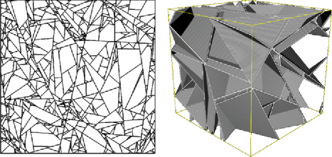
Figure 1: Simulations of a planar and a spatial stationary and isotropic STIT tessellation (kindly provided by Joachim Ohser and Claudia Redenbach).

Having studied the first- and second-order properties of STIT tessellations in STP1 , STP2 , we consider in this paper the central limit problem. This problem will be approached in two closely related settings, interestingly leading to results of very different qualitative nature. First, we shall focus our interest on the residual length/surface increment process, arising, respectively, as cumulative length or surface area of the cell-separating $(d-1)$-polyhedral facets born after a certain fixed initial time in the course of the MNW-construction. In this set-up we shall establish a central limit theorem with a Gaussian limiting variable. Next, we shall pass to the total length/surface, taking into account also the segments/facets born at the very initial big bang stages of the MNW-construction, as descriptively termed in MNW . It turns out that, whereas in dimension $2$ the Gaussian convergence is preserved, this is no more the case for dimensions $3$ and higher, where non-Gaussian limits arise. This apparently surprising phenomenon is in fact due to the influence of the big bang phase in the MNW-construction itself, which is negligible in the planar case, but turns out to be crucial in higher dimensions.

We are now going to describe some of our limit theorems in more detail. For a compact convex set $W$ as above, we put $W_{R}:=RW$ for $R>0$ and let $\Lambda$ be some fixed hyperplane measure as in (1). Therefore and in order to simplify the notation we will write from now on $Y(t,W)$ instead of $Y(t\Lambda,W)$. Our first limit theorem deals with the total surface area $\operatorname{Vol}_{d-1}(Y(t,W))$ of cell boundaries induced by the MNW-construction within the time period $[s_{0},1]$, where $0<s_{0}<1$ is some positive initial time moment.

Theorem 1

For each $0<s_{0}<1$, the random variable

$$\frac{1}{R^{d/2}}\bigl{[}\bigl{(}{\operatorname{Vol}}_{d-1}(Y(1,W_{R}))-\mathbb{E}{\operatorname{Vol}}_{d-1}(Y(1,W_{R}))\bigr{)}$$

$$\qquad{}-\bigl{(}{\operatorname{Vol}}_{d-1}(Y(s_{0},W_{R}))-\mathbb{E}{\operatorname{Vol}}_{d-1}(Y(s_{0},W_{R}))\bigr{)}\bigr{]}$$

converges, as $R\rightarrow\infty$, in law to $\mathcal{N}(0,V_{W}(\operatorname{Vol}_{d-1},\Lambda)\int_{s_{0}}^{1}s^{1-d}\,ds)$, a normal distribution with mean $0$ and variance $V_{W}(\operatorname{Vol}_{d-1},\Lambda)\int_{s_{0}}^{1}s^{1-d}\,ds$, where$V_{W}(\operatorname{Vol}_{d-1},\Lambda)$ is explicitly given by (3) or alternatively (17) below.

This statement cannot be extended to $s_{0}\downarrow 0$, as would be of interest as potentially leading to a Gaussian limit for the (centered and suitably normalized) total edge length/surface area ${\operatorname{Vol}}_{d-1}(Y(1,W_{R})).$ The problem is that the variance integral $V_{W}(\operatorname{Vol}_{d-1},\Lambda)\int_{s_{0}}^{t}s^{1-d}\,ds$ diverges at $0.$ However, this difficulty can be overcome for $d=2$, but not for $d>2$. Indeed, in the planar case the asymptotic behavior of the total edge length turns out to be Gaussian:

Theorem 2

For a STIT tessellation $Y(1,W_{R})$ in the plane we have

$$\frac{1}{R\sqrt{\log R}}[{\operatorname{Vol}}_{1}(Y(1,W_{R}))-\mathbb{E}{\operatorname{Vol}}_{1}(Y(1,W_{R}))]\Longrightarrow\mathcal{N}(0,V_{W}(\operatorname{Vol}_{1},\Lambda)),$$

where $\Longrightarrow$ means convergence in law and where again $V_{W}(\operatorname{Vol}_{1},\Lambda)$ is explicitly known and given by (3) or (17) below.

In fact, Theorems 1 and 2 are direct consequences of our much stronger functional central limit theorems, Theorems 4 and 5 below.

For space dimensions $d>2$ we claim that the Gaussian convergence cannot be preserved. Even though we are able to show this fact for all $W$ and translation invariant $\Lambda$ by establishing non-Gaussian tail decay, for simplicity, and in order to keep the argument transparent, we only give a proof for a more easily tractable particular case, in which all cells have the shape of cuboids (rectangular parallelepipeds). The study of more involved properties of the resulting random field is postponed to a future paper.

Theorem 3

Fix $d>2$, take $W=[0,1]^{d}$ and consider the hyperplane measure

$$\Lambda:=(2d)^{-1}\sum_{i=1}^{d}\int_{-\infty}^{+\infty}\delta_{re_{i}+e_{i}^{\bot}}\,dr,$$ (2)

where $e_{i},i=1,\ldots,d$ are vectors of the standard orthonormal basis for $\mathbb{R}^{d}$ and $\delta_{re_{i}+e_{i}^{\bot}}$ is the unit mass concentrated on the hyperplane orthogonal to $e_{i}$ at distance $r$ from the origin (here $e_{i}^{\bot}$ stands for the orthogonal complement of $e_{i}$). In this setting,

$${1\over R^{d-1}}[{\operatorname{Vol}}_{d-1}(1,W_{R})-\mathbb{E}{\operatorname{Vol}}_{d-1}(1,W_{R})]$$

converges, as $R\rightarrow\infty$, to a non-Gaussian square-integrable random variable $\Xi(W)$ with explicitly known variance given by (3) below.

The paper is structured as follows: In the next section we recall some properties of STIT tessellations needed for the proofs of our limit theorems. We also recall there some of the facts from STP1 , STP2 in order to keep the paper self-contained and present the exact statements of our functional central limit theorems. The proofs of our results are the content of Section 3.

We would like to remark that an extended version ST of this text is available online and, moreover, that the results in the present paper form the basis of our works ST2 , ST3 .

2 Background material and statement of the functional limit theorems

We start by rephrasing some of the properties of the STIT tessellations $Y(t\Lambda,W)$ as defined in the introduction, the proofs of which may be found in NW05 :

• $Y(t\Lambda,W)$ is consistent in that $Y(t\Lambda,W)\cap V\stackrel{{\scriptstyle D}}{{=}}Y(t\Lambda,V)$ for convex $V\subset W$ (here and below $\stackrel{{\scriptstyle D}}{{=}}$ stands for equality in distribution) and thus $Y(t\Lambda,W)$ can be extended to a random tessellation $Y(t\Lambda)$ in the whole space $\mathbb{R}^{d}$ such that $Y(t\Lambda)\cap W$ has the same distribution as $Y(t\Lambda,W)$.

  This way, instead of interpreting $Y(t\Lambda,W)$ as outcome of the MNW-construction carried out in $W$, $Y(t\Lambda,W)$ can also be understood as restriction of the whole space random tessellation $Y(t\Lambda)$ (which is a proper tessellation in the usual sense of stochastic geometry as discussed in the introduction) to the window $W$.

• $Y(t\Lambda)$ is a stationary random tessellation, that is, stochastically translation invariant. If, moreover, $\Lambda$ is the isometry-invariant hyperplane measure $\Lambda_{\mathrm{iso}}$, or equivalently if $\mathcal{R}$ in (1) is the uniform distribution $\nu_{d-1}$ on $\mathcal{S}_{d-1}$, then $Y(t\Lambda_{\mathrm{iso}})$ is even isotropic, that is, stochastically invariant under rotations around the origin.

• $Y(t\Lambda)$ is stable under the operation of iteration, denoted by $\boxplus$. This is to say

  $$Y(t\Lambda)\stackrel{{\scriptstyle D}}{{=}}m\bigl{(}Y\bigl{(}(t/m)\Lambda\bigr{)}\boxplus\cdots\boxplus Y\bigl{(}(t/m)\Lambda\bigr{)}\bigr{)}\qquad m=2,3,\ldots.$$

  For this reason, $Y(t\Lambda)$ is called a random STIT tessellation. This property was discussed in detail in NW05 , STP1 , and we refer to these papers and the references cited therein for further discussion, because our arguments do not explicitly use the stochastic stability, but its consequences.

• The surface density of $Y(t\Lambda)$, that is, the mean surface area of cell boundaries of $Y(t\Lambda)$ per unit volume equals $t$. In particular, the mean surface area of facets arising in the MNW-construction during time $[0,t]$ within a compact convex $W\subset\mathbb{R}^{d}$ with interior points is given by $t\operatorname{Vol}_{d}(W)$.

• STIT tessellations enjoy the following scaling property:

  $$tY(t\Lambda)\stackrel{{\scriptstyle D}}{{=}}Y(\Lambda),$$

  that is, the tessellation $Y(t\Lambda)$ of surface density $t$ upon rescaling by factor $t$ has the same distribution as $Y(\Lambda)$, the STIT tessellation with surface density $1$.

• The intersection of a STIT tessellation in $\mathbb{R}^{d}$ with a $k$-dimensional affine subspace $L_{k}$ ($1\leq k\leq d-1$), that is independent of the tessellation induces a STIT tessellation in $L_{k}$.

• STIT tessellations have Poisson typical cells, which is to say that the distribution of the interior of the typical cell $\operatorname{TypicalCell}(Y(t\Lambda))$ of $Y(t\Lambda)$ coincides with that of a Poisson hyperplane tessellation $\operatorname{PHT}(t\Lambda)$ having intensity measure $t\Lambda$; see the discussion after Theorem 1 in STP1 or NW03 .

For the nonspecialized reader let us remark that the typical cell of a tessellation is what we get when we choose equiprobably a cell of the tessellation at random out of a “large” observation window. The exact definition makes use of Palm theory for which we refer to SW . Moreover, let us recall that a Poisson hyperplane tessellation $\operatorname{PHT}(t\Lambda)$ is a random subdivision of $\mathbb{R}^{d}$ induced by a Poisson point process on the space of hyperplanes $\mathcal{H}$ with intensity measure $t\Lambda$.

The finite volume continuous-time incremental MNW-construction of random STIT tessellations, as discussed in the Introduction, clearly has the Markov property in the continuous-time parameter, whence natural martingales arise, which will be of crucial importance for our further considerations. In fact, this observation was the starting point of STP1 , where a class of martingales associated to STIT tessellations was constructed. In order to streamline our discussion we do not repeat the full theory here, but rephrase the martingale property of two stochastic processes, on which the proofs of our limit theorems are based. To this end let $Y$ be some instant of $Y(t\Lambda,W)$, and let $\phi(\cdot)$ be a measurable facet functional of the form

$$\phi(f)=\operatorname{Vol}_{d-1}(f)\zeta(\vec{\mathbf{n}}(f))$$ (3)

with $\vec{\mathbf{n}}(f)$ standing for the unit normal to a facet $f$ and $\zeta$ for a bounded measurable function on $\mathcal{S}_{d-1}$. Moreover, denote the collection of cell-separating $(d-1)$-dimensional facets, usually referred to as $(d-1)$-dimensional maximal polytopes, arising in subsequent splits in the MNW-construction by $\operatorname{MaxPolytopes}_{d-1}(Y)$. (Note that some of these polytopes can be chopped-off by the possibly curved boundary of the convex window $W$ in which $Y$ is constructed and are no polytopes in the usual sense. However, we somehow abuse notation and remark that this technical issue causes no difficulties in our theory, because of the special form of the facet functional $\phi$.) Let us further define $\Sigma_{\phi}(Y)$ by

$$\Sigma_{\phi}(Y):=\sum_{f\in\operatorname{MaxPolytopes}_{d-1}(Y)}\phi(f)$$ (4)

and $A_{\phi^{2}}(Y)$ to be

$$A_{\phi^{2}}(Y):=\int_{[W]}\sum_{f\in\operatorname{Cells}(Y\cap H)}\phi^{2}(f)\Lambda(dH)$$

with $\operatorname{Cells}(Y\cap H)$ standing for the set of $(d-1)$-dimensional cells of the tessellation $Y\cap H$ induced by the intersection of $Y$ with a hyperplane $H$ (again, some of these cells may have a curved boundary, because of the intersection with the construction window). Let us further introduce the bar notation $\bar{\Sigma}_{\phi}(Y)$ for the centred version $\Sigma_{\phi}(Y)-\mathbb{E}\Sigma_{\phi}(Y)$ of $\Sigma_{\phi}(Y)$. Then, we have (see STP1 , STP2 ):

Proposition 1

The two stochastic processes

$$\bar{\Sigma}_{\phi}(Y(t\Lambda,W))\quad\mbox{and}\quad\bar{\Sigma}_{\phi}^{2}(Y(t\Lambda,W))-\int_{0}^{t}A_{\phi^{2}}(Y(s\Lambda,W))\,ds$$ (5)

are both $\Im_{t}$-martingales, where $\Im_{t}$ stands for the filtration generated by $(Y(s\Lambda,W))_{0\leq s\leq t}$.

In particular (see (LS, , Paragraph I.8)), by (5), the martingale $\bar{\Sigma}_{\phi}(Y(t\Lambda,W))$ has its predictable quadratic variation process $\langle\bar{\Sigma}_{\phi}(Y(\cdot,W))\rangle$ absolutely continuous (in the sense of functions) and given by

$$\langle\bar{\Sigma}_{\phi}(Y(\cdot,W))\rangle_{t}=\int_{0}^{t}A_{\phi^{2}}(Y(s\Lambda,W))\,ds.$$ (6)

Besides these martingale tools, we will also make use of the following formula for the variance $\operatorname{Var}(\Sigma_{\phi}(Y(t\Lambda,W)))$ of $\Sigma_{\phi}(Y(t\Lambda,W))$, $W\subset\mathbb{R}^{d}$ compact, convex and with interior points, established in full generality in STP2 , in order to calculate the variance of the limit random variable of our non-Gaussian limit theorem:

Proposition 2

For any nondegenerate translation-invariant $\Lambda$ of the form (1) and $\phi$ as in (3), we have

$$\operatorname{Var}\bigl{(}\Sigma_{\phi}(Y(t\Lambda,W))\bigr{)}$$

$$\qquad=\int_{[W]}\zeta^{2}(\vec{\mathbf{n}}(H))\int_{W\cap H}\int_{W\cap H}\frac{1-\exp(-t\Lambda([xy]))}{\Lambda([xy])}\,dx\,dy\Lambda(dH),$$

where $[xy]$ stands for the set of parameter values of hyperplanes hitting the line segment $xy$ connecting $x$ with $y$.

Let us further recall from STP2 that the variance of the total edge length of a stationary and isotropic STIT tessellation $Y(t\Lambda_{\mathrm{iso}},W_{R})$ in the plane behaves asymptotically like

$$\operatorname{Var}\bigl{(}\operatorname{Vol}_{1}(Y(t\Lambda_{\mathrm{iso}},W_{R}))\bigr{)}\sim\pi\operatorname{Vol}_{2}(W)R^{2}\log R\qquad\mbox{as }R\rightarrow\infty,$$ (7)

where $W$ is again a compact convex set as above. Indeed, this can be seen from the general statement in Proposition 2 combined with tools from integral geometry. Note that the asymptotic variance expression for the total edge length is independent of $t$. However, for all space dimensions $>2$, the surface density $t$ enters the asymptotic variance expression as shown in detail in STP2 .

We can now turn to the statement of our main results, the functional limit theorems, from which Theorems 1 and 2 are direct consequences. As in the Introduction we fix a hyperplane measure $\Lambda$ and suppress from now on the reference to $\Lambda$, for example by writing $Y(t,W_{R})$ instead of $Y(t\Lambda,W_{R})$.

Theorem 4

For each $0<s_{0}<1$ the centred surface increment process

$$\biggl{(}\mathcal{S}^{R,W}_{s_{0},t}:=\frac{1}{R^{d/2}}[\bar{\Sigma}_{\phi}(Y(t,W_{R}))-\bar{\Sigma}_{\phi}(Y(s_{0},W_{R}))]\biggr{)}_{t\in[s_{0},1]}$$

converges in law, as $R\to\infty,$ on the space $\mathcal{D}[s_{0},1]$ of right continuous functions with left-hand limits (càdlàg) on $[s_{0},1]$, endowed with the Skorokhod $J_{1}$-topology (LS, , Chapter 6.1), to a time-changed Wiener process

$$t\mapsto\mathcal{W}_{V_{W}(\phi,\Lambda)\int_{s_{0}}^{t}s^{1-d}\,ds},$$

where $\mathcal{W}_{(\cdot)}$ is the standard Wiener process, and $V_{W}(\phi,\Lambda)$ is given by (3), or alternatively (17), below. In particular,

$$\mathcal{S}^{R,W}_{s_{0},1}=\frac{1}{R^{d/2}}[\bar{\Sigma}_{\phi}(Y(1,W_{R}))-\bar{\Sigma}_{\phi}(Y(s_{0},W_{R}))]$$

converges in law to $\mathcal{N}(0,V_{W}(\phi,\Lambda)\int_{s_{0}}^{1}s^{1-d}\,ds)$, a normal distribution with mean $0$ and variance $V_{W}(\phi,\Lambda)\int_{s_{0}}^{1}s^{1-d}\,ds$.

We turn now to the functional convergence of the total length process in the planar case. Write

$$\tau(s,R):=\exp\bigl{(}[\log R-\log\log R](s-1)\bigr{)}=R^{s-1}(\log R)^{1-s},$$

and define the total length process

$$\mathcal{L}^{R,W}_{s}:=\frac{1}{R\sqrt{\log R}}\bar{\Sigma}_{\phi}(Y(\tau(s,R),W_{R})),\qquad s\in[0,1].$$

Theorem 5

The total length process $(\mathcal{L}^{R,W}_{s})_{s\in[0,1]}$ converges in law, as $R\to\infty,$ on the space $\mathcal{D}[0,1]$ of càdlàg functions on $[0,1]$, endowed with the Skorokhod $J_{1}$-topology, to $(\sqrt{V_{W}(\phi,\Lambda)}\mathcal{W}_{s})_{s\in[0,1]}$, where, again, $\mathcal{W}_{(\cdot)}$ stands for the standard Wiener process. In particular, $(R\sqrt{\log R})^{-1}\bar{\Sigma}_{\phi}(Y(1,W_{R}))$ converges in law to $\mathcal{N}(0,V_{W}(\phi,\Lambda))$ with, again, $V_{W}(\phi,\Lambda)$ given by (3) or (17).

Remark 1.

We consider in this paper facet functionals of the form $\phi(\cdot)=\operatorname{Vol}_{d-1}(\cdot)\zeta(\vec{\mathbf{n}}(\cdot))$; see (3). Taking $\zeta\equiv 1$, Theorems 4–5 reduce to the total surface area case discussed in Theorems 1 and 2 in the Introduction. However, the additional flexibility induced by the introduction of $\zeta(\cdot)$ implies that our results allow us to conclude limit theorems that are sensitive with respect to direction. Taking, for example, $\zeta(\cdot)=\mathbf{1}\{\vec{\mathbf{n}}(\cdot)\in U(n)\}$ to be the indicator function of a small neighborhood $U(n)$ of a fixed direction $n\in\mathcal{S}_{d-1}$ satisfying $\mathcal{R}(U(n))>0$ [recall the decomposition (1)], yields central limit theorems also for the collection of tessellation facets having their normals in $U(n)$. This means that our results are not only valid for the whole STIT tessellation, but also for parts in arbitrary space directions.

Remark 2.

So far we have restricted our considerations to space dimensions $d\geq 2$. STIT tessellations and their limit theory on the line can also be considered. However, in NW03 it was shown that a STIT tessellation on $\mathbb{R}$ is nothing than a homogeneous Poisson point process, or more precisely the intervals between its points. These point processes and their limit theory are well known, and for this reason we have focused on the cases $d\geq 2$.

3 Proofs

After having rephrased some background material on STIT tessellations in the previous section, we are now prepared to present the proofs of our limit theorems. Let us briefly recall that we will deal with a fixed translation-invariant hyperplane measure $\Lambda$, and for this reason we shall write, for example, $Y(t)$ instead of $Y(t\Lambda)$ without confusion. Moreover, we fix some compact and convex set $W\subset\mathbb{R}^{d}$ having interior points and write $W_{R}=RW$ for $W$ dilated by a factor $R>0$. Moreover, recall that the facet functionals we are dealing with have the representation (3), that $\Sigma_{\phi}(Y(t))$ was defined in (4) and that the bar notation $\bar{\Sigma}_{\phi}(Y(t))$ stands for the centered version $\Sigma_{\phi}(Y(t))-\mathbb{E}\Sigma_{\phi}(Y(t))$. Proof of Theorem 4 Notice first that because of $\Lambda([W_{R}])=R\Lambda([W])$, we have

$$\frac{1}{R^{d}}A_{\phi^{2}}(Y(1,W_{R}))$$

$$\qquad=\frac{1}{R}\int_{[W_{R}]}\frac{1}{R^{d-1}}\zeta^{2}(\vec{\mathbf{n}}(H))\sum_{f\in\operatorname{Cells}(Y(1,W_{R})\cap H)}\operatorname{Vol}^{2}_{d-1}(f)\Lambda(dH)$$ (8)

$$\qquad=\int_{[W]}\frac{1}{R^{d-1}}\zeta^{2}(\vec{\mathbf{n}}(H))\sum_{f\in\operatorname{Cells}(Y(1,W_{R})\cap RH)}\operatorname{Vol}^{2}_{d-1}(f)\Lambda(dH).$$

We claim that, upon letting $R\to\infty$, this converges in probability to

$$V_{W}(\phi,\Lambda)$$

$$\qquad:=\int_{[W]}\zeta^{2}(\vec{\mathbf{n}}(H))\operatorname{Vol}_{d-1}(W\cap H)$$

(9)

$$\qquad{}\hskip 32.0pt\times\frac{\mathbb{E}\operatorname{Vol}^{2}_{d-1}(\operatorname{TypicalCell}(Y(1)\cap H))}{\mathbb{E}\operatorname{Vol}_{d-1}(\operatorname{TypicalCell}(Y(1)\cap H))}\Lambda(dH)$$

$$\qquad=\operatorname{Vol}_{d}(W)\int_{\mathcal{S}_{d-1}}\zeta^{2}(u)\frac{\mathbb{E}\operatorname{Vol}^{2}_{d-1}(\operatorname{TypicalCell}(Y(1)\cap u^{\bot}))}{\mathbb{E}\operatorname{Vol}_{d-1}(\operatorname{TypicalCell}(Y(1)\cap u^{\bot}))}\mathcal{R}(du),$$

where $\mathcal{R}$ is the directional distribution of the tessellation as given by (1). To see it, recall that $Y(1)\cap RH$ is a STIT tessellation in $RH$ for each $R>0$ and $H\in\mathcal{H}.$ Thus, applying (SW, , (4.6) and Theorem 4.1.3) to this tessellation and the fact that $\mathbb{E}\operatorname{Vol}_{d}(\operatorname{TypicalCell}(Y(1)\cap u^{\perp}))$ is the same as the inverse cell density of the tessellation $Y(1)\cap u^{\perp}$ [see (10.4) ibidem], we get

$$\lim_{R\to\infty}\frac{1}{R^{d-1}}\mathbb{E}\sum_{f\in\operatorname{Cells}(Y(1,W_{R})\cap RH)}\operatorname{Vol}^{2}_{d-1}(f)$$

(10)

$$\qquad=\operatorname{Vol}_{d-1}(W\cap H)\frac{\mathbb{E}\operatorname{Vol}^{2}_{d-1}(\operatorname{TypicalCell}(Y(1)\cap H))}{\mathbb{E}\operatorname{Vol}_{d-1}(\operatorname{TypicalCell}(Y(1)\cap H))}.$$

Next, we observe that $Y(1,W_{R})\cap RH\stackrel{{\scriptstyle D}}{{=}}Y(1)\cap R\cdot_{H}(H\cap W)$, where $\cdot_{H}$ is the scalar multiplication relative in $H$, that is, to say, $H\ni R\cdot_{H}x=p_{H}(0)+R(x-p_{H}(0)),x\in H$ with $p_{H}$ standing for the orthogonal projection on $H.$ Thus, using the recently developed strong mixing and tail triviality theory for STIT tessellations, especially (LR, , Theorem 2), noting that tail trivial stationary processes are ergodic (GEO, , Proposition 14.9) and then applying the multidimensional ergodic theorem (see, e.g., Corollary 14.A5 ibidem), to $\frac{1}{R^{d-1}}\sum_{f\in\operatorname{Cells}(Y(1)\cap R\cdot_{H}(H\cap W))}\operatorname{Vol}^{2}_{d-1}(f),$ we get from (3) that

$$\lim_{R\to\infty}\frac{1}{R^{d-1}}\sum_{f\in\operatorname{Cells}(Y(1,W_{R})\cap RH)}\operatorname{Vol}^{2}_{d-1}(f)$$

$$\qquad=\operatorname{Vol}_{d-1}(W\cap H)\frac{\mathbb{E}\operatorname{Vol}^{2}_{d-1}(\operatorname{TypicalCell}(Y(1)\cap H))}{\mathbb{E}\operatorname{Vol}_{d-1}(\operatorname{TypicalCell}(Y(1)\cap H))}$$

in probability. Putting this together with (3) and integrating over $[W]$ yields

$$\lim_{R\to\infty}\frac{1}{R^{d}}A_{\phi^{2}}(Y(1,W_{R}))=V_{W}(\phi,\Lambda)\qquad\mbox{in probability},$$ (11)

as required.

Note now that by the scaling properties of $Y(s,W_{R})$ and $\phi^{2}$ for $s>0$, we have

$$\frac{1}{R^{d}}A_{\phi^{2}}(Y(s,W_{R})) \stackrel{{\scriptstyle D}}{{=}} \frac{1}{R^{d}s^{2d-1}}A_{\phi^{2}}(Y(1,W_{sR}))$$

$$\stackrel{{\scriptstyle D}}{{=}} \frac{1}{s^{d-1}}\frac{1}{(Rs)^{d}}A_{\phi^{2}}(Y(1,W_{sR})).$$

Thus, combining (11) with the scaling relation (3), we get

$$\lim_{R\to\infty}\frac{1}{R^{d}}A_{\phi^{2}}(Y(s,W_{R}))=\frac{1}{s^{d-1}}V_{W}(\phi,\Lambda)$$ (13)

in probability and uniformly in $s\in[s_{0},1].$

This crucial statement puts us now in context of general martingale limit theory. Indeed, using Propositon 1, we see that

$$\mathcal{S}^{R,W}_{s_{0},s}=\frac{1}{R^{d/2}}[\bar{\Sigma}_{\phi}(Y(1,W_{R}))-\bar{\Sigma}_{\phi}(Y(s_{0},W_{R}))]$$

is a martingale with absolutely continuous predictable quadratic variation process

$$\langle\mathcal{S}^{R,W}_{s_{0},\cdot}\rangle_{t}=\int_{s_{0}}^{t}\frac{1}{R^{d}}A_{\phi^{2}}(Y(s,W_{R}))\,ds$$ (14)

by (5) and (11); see again Paragraph I.8 in LS . In these terms, (13) yields for each $t$,

$$\lim_{R\to\infty}\langle\mathcal{S}^{R,W}_{s_{0},\cdot}\rangle_{t}=\int_{s_{0}}^{t}\frac{1}{s^{d-1}}V_{W}(\phi,\Lambda)\,ds\qquad\mbox{in probability. }$$ (15)

We now want to apply the martingale functional central limit theorem. Whereas this is well known for continuous martingales, we need a version for martingales in the Skorokhod space $\mathcal{D}[s_{0},1]$. In this paper, we will make use of the version formulated as Theorem 2.1 in the survey article WW . In order to apply this theorem, several conditions have to be checked. Condition (ii.6) in [WW , Theorem 2.1] is just (15), whereas condition (ii.4) there is trivially verified, because the predictable quadratic variation $\langle\mathcal{S}^{R,W}_{s_{0},\cdot}\rangle$ has no jumps by (14). It remains to check condition (ii.5) ibidem, which is that the second moment of the maximum jump $\mathcal{J}(\mathcal{S}^{R,W}_{s_{0},\cdot};1)$ of the process $(\mathcal{S}^{R,W}_{s_{0},s})_{s\in[s_{0},1]}$ goes to $0$, as $R\to\infty.$ More precisely,

$$\mathcal{J}(\mathcal{S}^{R,W}_{s_{0},\cdot};1)=\sup_{s_{0}\leq t\leq 1}|\mathcal{S}^{R,W}_{s_{0},t}-\mathcal{S}^{R,W}_{s_{0},t-}|,\qquad\mathcal{S}^{R,W}_{s_{0},t-}=\lim_{s\uparrow t}\mathcal{S}^{R,W}_{s_{0},s},$$

and we have to check that

$$\lim_{R\rightarrow\infty}\mathbb{E}\mathcal{J}^{2}(\mathcal{S}^{R,W}_{s_{0},\cdot};1)=0.$$

To this end, note first that, with probability one, $\mathcal{J}(\mathcal{S}^{R,W}_{s_{0},\cdot};1)$ is bounded from above by a constant multiple of $R^{-d/2}$ times the $(d-1)$th power of the diameter of the largest cell of $Y(s_{0},W_{R}).$ Since the typical cell distribution of $Y(s_{0})$ is the same as that of a Poisson hyperplane tessellation with intensity measure $s_{0}\Lambda$ (see Theorem 1 in STP1 or Section 2 above), we conclude by standard properties of Poisson hyperplane tessellations that the expected number $e(Y(s_{0},W_{R}),D)$ of cells in $Y(s_{0},W_{R})$ with diameter exceeding $D$ is of order $O(R^{d}\exp(-D))$. To see it, write $\operatorname{diam}(c)$ for the diameter of a cell $c$ and $\mathbf{1}\{\cdot\}$ for the usual indicator function and rewrite $e(Y(s_{0},W_{R}),D)$ as

$$e(Y(s_{0},W_{R}),D)=\mathbb{E}\sum_{c\in\operatorname{Cells}(Y(s_{0},W_{R}))}\mathbf{1}\{\operatorname{diam}(c)>D\},$$

which by Theorem 4.1.3 in SW is of the same order as the mean number $N(Y(s_{0},W_{R}))=\mathbb{E}\sum_{c\in\operatorname{Cells}(Y(s_{0},W_{R}))}1$ of cells in $Y(s_{0},W_{R})$ times the probability that the typical cell diameter of $Y(s_{0})$ exceeds $D$ (the additional condition in Theorem 4.3.1 in SW is easily verified by using Steiner’s formula together with the fact that the typical cell of a Poisson hyperplane tessellation has finite mean intrinsic volumes; see Theorem 10.3.3 ibidem). Thus, $e(Y(s_{0},W_{R}),D)$ satisfies

$$e(Y(s_{0},W_{R}),D)=O\bigl{(}N(Y(s_{0},W_{R}))\mathbb{P}\bigl{(}\operatorname{diam}(\operatorname{TypicalCell}(Y(s_{0})))>D\bigr{)}\bigr{)}.$$

Stationarity of the tessellation implies that the first factor is of volume order $R^{d}$. We claim that the second term is bounded from above by $c_{1}e^{-c_{2}s_{0}D}$, where $c_{1}$ and $c_{2}$ are constants which depend on the hyperplane measure $\Lambda$. To this end we notice first that the typical cell of $Y(s_{0})$ is stochastically smaller than the almost surely uniquely determined cell $Z_{0}$ of $Y(s_{0})$ containing the origin; cf. Corollary 10.4.1 in SW . Moreover, equation (20) in HS1 with $\Sigma=\operatorname{diam}$, $\varepsilon=0$ and $\alpha=1$ there (the other parameters are then $k=\tau=1$) implies that there are constants $c_{1},c_{2}>0$ depending on the hyperplane measure $\Lambda$ such that $\mathbb{P}(\operatorname{diam}(Z_{0})>D)\leq c_{1}e^{-c_{2}s_{0}D}$. This implies

$$\mathbb{P}\bigl{(}\operatorname{diam}\bigl{(}\operatorname{TypicalCell}(Y(s_{0}))\bigr{)}>D\bigr{)}\leq\mathbb{P}\bigl{(}\operatorname{diam}(Z_{0})>D\bigr{)}\leq c_{1}e^{-c_{2}s_{0}D}.$$

Putting these two issues together leads to the desired order $O(R^{d}\exp(-D))$ for the expected number of cells in $Y(s_{0},W_{R})$ with diameter exceeding $D$. Recalling that $\mathcal{J}(\mathcal{S}^{R,W}_{s_{0},\cdot};1)$ is bounded from above by a constant multiple of $R^{-d/2}$ times the $(d-1)$th power of the diameter of the largest cell of $Y(s_{0},W_{R})$, and putting $u=D^{d-1}R^{-d/2}$ we find

$$\mathbb{P}\bigl{(}\mathcal{J}(\mathcal{S}^{R,W}_{s_{0},\cdot};1)>u\bigr{)}=O\bigl{(}R^{d}\exp\bigl{(}-R^{d/(2d-2)}u^{1/(d-1)}\bigr{)}\bigr{)}.$$ (16)

Clearly, (16) is sufficient to guarantee that

$$\lim_{R\to\infty}\mathbb{E}\mathcal{J}^{2}(\mathcal{S}^{R,W}_{s_{0},\cdot};1)=0,$$

which gives the required condition (ii.5) of Theorem 2.1 in WW . This result yields now the functional convergence as stated in our Theorem 4.

Before turning to the proof of Theorem 5 we provide an alternative formula for the factor $V_{W}(\phi,\Lambda)$. Readers not specialized in convex or stochastic geometry could also skip this alternative representation and directly jump to the next paragraph, because Proposition 3 will not be used in the sequel. However, having such a more explicit variance expression is useful for other purposes and has already been used in our work ST3 . We denote, as in SW or STP1 , by $\Pi$ the associated zonoid of a Poisson hyperplane tessellation with intensity measure $\Lambda$, by $\Pi^{o}$ its polar body and by $\mathcal{R}$ the directional distribution of the STIT tessellation from (1); see SW for the precise definitions of $\Pi$ and $\Pi^{o}$.

Proposition 3

We have

$$V_{W}(\phi,\Lambda)=\operatorname{Vol}_{d}(W){(d-1)!\over 2^{d-1}}\int_{\mathcal{S}_{d-1}}\zeta^{2}(u)\operatorname{Vol}_{d-1}((\Pi|u^{\perp})^{o})\mathcal{R}(du),$$ (17)

where $\Pi|u^{\perp}$ stands for the orthogonal projection of $\Pi$ onto the hyperplane $u^{\perp}$, and where the polar body $(\Pi|u^{\perp})^{o}$ is considered relative to $u^{\perp}.$ In the isotropic case, that is, when $\mathcal{R}=\nu_{d-1}$, the uniform distribution on the unit sphere $\mathcal{S}_{d-1}$, this reduces to

$$V_{W}(\phi,\Lambda_{\mathrm{iso}})=\operatorname{Vol}_{d}(W)2^{d-1}\pi^{d-{3/2}}{\Gamma({(d+1)/2})^{d-1}\over\Gamma({d/2})^{d-2}}\int_{\mathcal{S}_{d-1}}\zeta^{2}(u)\nu_{d-1}(du).$$

In particular for $\zeta\equiv 1$, $W=B_{1}^{d}$ the unit ball and $d=2$ and $d=3$, we conclude the exact values

$$V_{B_{1}^{2}}(\operatorname{Vol}_{1},\Lambda_{\mathrm{iso}})=\pi^{2}\quad\mbox{and}\quad V_{B_{1}^{3}}(\operatorname{Vol}_{2},\Lambda_{\mathrm{iso}})={32\over 3}\pi^{2}.$$

At first, FW , Corollary 3.7, provides a general formula for the second moment of the volume of the typical Poisson cell of a stationary Poisson hyperplane tessellation $\operatorname{PHT}(\Lambda)$ in $\mathbb{R}^{d}$ having intensity measure $\Lambda$. In terms of the zonoid $\Pi$ it reads

$$\mathbb{E}\operatorname{Vol}_{d}^{2}(\operatorname{TypicalCell}(\operatorname{PHT}(\Lambda)))={d!\over 2^{d}}{\operatorname{Vol}_{d}(\Pi^{o})\over\operatorname{Vol}_{d}(\Pi)},$$

where we have used [SW , equation (4.63)]. Moreover, the first volume moment of the typical cell of a Poisson hyperplane tessellation with intensity measure $\Lambda$ equals $1/\operatorname{Vol}_{d}(\Pi)$ according to [SW , Theorem 10.3.3 and (10.4)]. Using now equation (4.61) ibidem and the fact that STIT tessellations have Poisson typical cell distributions and replacing $d$ by $d-1$ in the last two formulas, we obtain (17) immediately from (3). The precise value in the stationary and isotropic case can be calculated from the fact that in this case, $\Pi$ is a ball with a known radius; see SW .

Proof of Theorem 5 Recall that $\tau(s,R)$ is defined by

$$\tau(s,R)=\exp\bigl{(}[\log R-\log\log R](s-1)\bigr{)}=R^{s-1}(\log R)^{1-s},$$

and note that this implies

$$\tau(0,R) = \frac{\log R}{R},\qquad\tau(1,R)=1,$$

$$\frac{\partial}{\partial s}\tau(s,R) = \tau(s,R)[\log R-\log\log R].$$

Thus, defining the auxiliary process

$$M^{R,W}_{s} = M_{s}$$

$$:= \frac{1}{R\sqrt{\log R-\log\log R}}[\bar{\Sigma}_{\phi}(Y(\tau(s,R),W_{R}))-\bar{\Sigma}_{\phi}(Y(\tau(0,R),W_{R}))]$$

and using (5) with $W_{R}:=RW$ and under variable substitution $s:=\tau(u,R)$ and $t:=s,$ with left-hand side variables corresponding to the notation of (5), and those on the right-hand side to that used here, we see that, by (3),

$$(M_{s})_{s\in[0,1]}\quad\mbox{and}\quad\biggl{(}M^{2}_{s}-\int_{0}^{s}\frac{\tau(u,R)}{R^{2}}A_{\phi^{2}}(Y(\tau(u,R),W_{R}))\,du\biggr{)}_{s\in[0,1]}$$

are $\Im_{\tau(s,R)}$-martingales. In particular (see, once more, (LS, , Paragraph I.8)), the predictable quadratic variation process $\langle M\rangle_{s}$ is given by

$$\langle M\rangle_{s}=\int_{0}^{s}\frac{\tau(u,R)}{R^{2}}A_{\phi^{2}}(Y(\tau(u,R),W_{R}))\,du,\qquad s\in[0,1].$$ (19)

Repeating the argument leading to (13) we see that

$$\lim_{R\to\infty}\frac{\tau(s,R)}{R^{2}}A_{\phi^{2}}(Y(\tau(s,R),W_{R}))=V_{W}(\phi,\Lambda)$$ (20)

in probability and uniformly in $s\in[0,1].$ Note that the uniformity in $s$ comes, as in the case of (13), from the relation (3) implying that, in distribution, all instances of the left-hand side for different values of $s$ are just re-scalings of the same object $\tilde{R}^{-2}A_{\phi^{2}}(Y(1,W_{\tilde{R}}))$ for $\tilde{R}=R/\tau(s,R)$, and thus, in terms of the considered convergence in probability to a deterministic limit, we are just dealing with a single asymptotic statement. Consequently, by (20) and in full analogy to (15),

$$\lim_{R\to\infty}\langle M\rangle_{s}=\int_{0}^{s}V_{W}(\phi,\Lambda)\,du=sV_{W}(\phi,\Lambda)\qquad\mbox{in probability.}$$ (21)

Thus, we are again in a position to apply the martingale functional central limit theorem (WW, , Theorem 2.1) yielding the functional convergence in law, as $R\to\infty,$ in $\mathcal{D}[0,1]$ of $(M_{s})_{s\in[0,1]}$ to the random process $(\sqrt{V_{W}(\phi,\Lambda)}\mathcal{W}_{s})_{s\in[0,1]}.$ Indeed, condition (ii.6) there is just (21), condition (ii.4) is trivial in view of (19), whereas the condition (ii.5) is verified by noting that, with probability one, $\mathcal{J}(M;1)=\frac{1}{R\sqrt{\log R}}O(R\operatorname{diam}(W))=O(1/\sqrt{\log R})$, so that in particular

$$\lim_{R\to\infty}\mathbb{E}\mathcal{J}^{2}(M;1)=0,$$

as required.

Denoting now by $C^{R,W}$ the correction term ${1\over R\sqrt{\log R}}\bar{\Sigma}_{\phi}(Y(\tau(0,R),W_{R})),$ such that

$$\mathcal{L}^{R,W}_{s}=C^{R,W}+\sqrt{\frac{\log R-\log\log R}{\log R}}M_{s},$$

noting that $\log R-\log\log R\sim\log R$ and that, by the scaling property of STIT tessellations and by (7),

$$\operatorname{Var}(C^{W,R}) = O\bigl{(}[R^{-2}(\log R)^{-1}][R^{2}/(\log R)^{2}][(\log R)^{2}(\log\log R)]\bigr{)}$$

$$= O(\log\log R/\log R),$$

we see that the processes $M_{s}$ and $\mathcal{L}^{R,W}_{s}$ are asymptotically equivalent in $\mathcal{D}[0,1]$, as $R\to\infty.$ This completes the proof of Theorem 5.

Remark 3.

In the context of proof of Theorem 5 it should be remarked that the “negligible correction term” $C^{R,W}$ has its variance of order

$$O(\log\log R/\log R)$$

and is thus indeed tending to $0,$ but extremely slowly. Consequently, although the Gaussian CLT holds for $\mathcal{L}^{R,W}_{1},$ it is quite natural to expect that the convergence rates are extremely slow and conjecturedly logarithmic. This is due to the fact that dimension $2$ is the largest dimension (critical dimension) where the Gaussian limits are still present. In dimensions $3$ and higher there is no Gaussian CLT and the “correction term” analogous to $C^{R,W}$ will turn out order-determining rather than negligible, as shown by Theorem 3.

We turn now to the higher-dimensional situations. Even if in the formulation of Theorem 3 we have used the surface area functional, we will show the statement in a more general context, where ${\operatorname{Vol}}_{d-1}(Y(1,W_{R}))$ is replaced by a general cumulative facet functional $\Sigma_{\phi}(Y(1,W_{R}))$ satisfying (3).

We claim that the argument from the proof of Theorem 5 cannot be repeated for $d>2.$ Intuitively, this is due to the fact that for $d>2$ the variance order of $\bar{\Sigma}_{\phi}(Y(1,W_{R}))$ is $O(R^{2(d-1)})$, see below, whereas the variance order of the increment $\bar{\Sigma}_{\phi}(Y(1,W_{R}))-\bar{\Sigma}_{\phi}(Y(s_{0},W_{R}))$, with some time instant $0<s_{0}<1$, is $O(R^{d})$ as seen from Theorem 4. Hence, for $d>2$ we conclude that even the very first facets born in the MNW-cell-division process already bring a nonnegligible contribution to the overall variance. Thus, we cannot split the whole STIT construction into the warm-up phase ($t\in[0,R^{-1}\log R]$ for $d=2$) with negligible variance contribution and the proper phase unfolding already in a typical STIT environment. In fact, the claim is that the CLT does not hold for STIT surface functionals in dimension greater than $2!$

Proof of Theorem 3 Recall that we do not show this fact in full generality for all nondegenerate hyperplane measures $\Lambda$ and all windows $W$, but restrict ourself to a particular case, where $\Lambda$ is given by (2) and where $W=[0,1]^{d}$. To see the non-Gaussianity, observe first that, by the scaling property of STIT tessellations,

$$R^{-(d-1)}\bar{\Sigma}_{\phi}(Y(1,W_{R}))\stackrel{{\scriptstyle D}}{{=}}\bar{\Sigma}_{\phi}(Y(R,W)),$$ (22)

which implies that the variance $\operatorname{Var}(\Sigma_{\phi}(Y(1,W_{R})))$ is of order $O(R^{2(d-1)})$. Indeed, this follows directly from the special form (3) of the facet functional $\phi$ and the scaling relation $Y(1,W_{R})\stackrel{{\scriptstyle D}}{{=}}RY(R,W)$. Further, recall that by (5) the process $R\mapsto\bar{\Sigma}_{\phi}(Y(R,W))$ is a square-integrable martingale with absolutely continuous predictable quadratic variation process given as in (6). Moreover, by Proposition 2 we conclude

$$\operatorname{Var}\bigl{(}\Sigma_{\phi}(Y(R,W))\bigr{)}$$

$$\qquad=\int_{[W]}\zeta^{2}(\vec{\mathbf{n}}(H))\int_{W\cap H}\int_{W\cap H}\frac{1-\exp(-R\Lambda([xy]))}{\Lambda([xy])}\,dx\,dy\Lambda(dH),$$

which is bounded uniformly in $R.$ Consequently, by the martingale convergence theorem (cf. Corollary 7.22 in K ) there exists a centered square-integrable random variable $\Xi(W)$ such that

$$\Xi(W)=\lim_{R\to\infty}\bar{\Sigma}_{\phi}(Y(R,W))$$

a.s. and in $L^{2}$ and, moreover,

$$\operatorname{Var}(\Xi(W)) = \lim_{R\rightarrow\infty}\operatorname{Var}\bigl{(}\Sigma_{\phi}(Y(R,W))\bigr{)}$$

$$= \int_{[W]}\zeta^{2}(\vec{\mathbf{n}}(H))\int_{W\cap H}\int_{W\cap H}\frac{1}{\Lambda([xy])}\,dx\,dy\Lambda(dH).$$

Using now (22) we readily conclude that

$$R^{-(d-1)}\bar{\Sigma}_{\phi}(Y(1,W))\Longrightarrow\Xi(W),$$

as $R\to\infty,$ where $\Longrightarrow$ stands for convergence in distribution.

We show now that the variable $\Xi(W)$ cannot be Gaussian. To see it, consider the event $\mathcal{E}_{N},N>0,$ that only hyperplanes orthogonal to $e_{1}$ have been born during time $[0,1]$ in the MNW-construction and that their number exceeds $N.$ Observe that, in view of the special form (2) of the hyperplane measure $\Lambda,$ $\mathbb{P}(\mathcal{E}_{N})=\exp(-d)\sum_{k=N+1}^{\infty}\frac{1}{k!}$ and thus

$$\mathbb{P}(\mathcal{E}_{N})=\exp(-\Theta(N\log N)),$$ (24)

where by $\Theta(\cdot)$ we mean a function bounded both from below and above by multiples of the argument. Further, given the fixed collection of all hyperplanes $H_{1},\ldots,H_{k}$ ($k>N$) born at times between $0$ and $1,$ on the event $\mathcal{E}_{N}$, we see that the conditional law of $\Xi(W)$ coincides with that of $k-d$ plus the sum of independent copies $\xi_{1},\ldots,\xi_{k+1}$ of $\Xi(W_{1}),\ldots,\Xi(W_{k+1})$ respectively, where $W_{j},j=1,\ldots,k+1,$ are the parallelepipeds into which $W=[0,1]^{d}$ is partitioned by $H_{1},\ldots,H_{k}$. More formally, we have the relation

$$\mathbb{P}\bigl{(}\Xi(W)>u|\mathcal{E}_{N,k}\bigr{)}=\mathbb{P}\bigl{(}k-d+(\xi_{1}+\cdots+\xi_{k+1})>u\bigr{)},\qquad u\in\mathbb{R},$$

where $\mathcal{E}_{N,k}$ is the event that exactly the hyperplanes $H_{1},\ldots,H_{k}$ ($k>N$) orthogonal to $e_{1}$ are born within time $[0,1]$. Note that the extra $k$ above is the sum of the $(d-1)$-volumes of $W\cap H_{i}$, whereas $-d=-\mathbb{E}\Sigma_{\phi}(Y(1,W))$ is the centering term.

Since $\operatorname{Var}(\xi_{1}+\cdots+\xi_{k+1})=\sum_{j=1}^{k+1}\operatorname{Var}(\Xi(W_{j}))$, which is bounded from above by $\operatorname{Var}(\Xi(W))$ in view of (3), by Chebyshev’s inequality we get

$$\mathbb{P}\bigl{(}\xi_{1}+\cdots+\xi_{k+1}\geq-2\sqrt{\operatorname{Var}(\Xi(W))}\bigr{)} \geq 1-{\operatorname{Var}(\xi_{1}+\cdots+\xi_{k+1})\over 4\operatorname{Var}(\Xi(W))}$$

$$\geq 1-{1\over 4}={3\over 4}.$$

Thus, in view of (24) we end up with

$$\mathbb{P}\bigl{(}\Xi(W)>N\bigr{)}\geq\frac{3}{4}\mathbb{P}\bigl{(}\mathcal{E}_{N+2\sqrt{\operatorname{Var}(\Xi(W))}+d}\bigr{)}=\exp(-\Theta(N\log N)).$$

Since Gaussian variables exhibit tail decay of the order $\exp(-\Theta(N^{2})),$ the random variable $\Xi(W)$ cannot be Gaussian.

References

- (1) {barticle}[mr] \bauthor\bsnmBaumstark, \bfnmVolker\binitsV. and \bauthor\bsnmLast, \bfnmGünter\binitsG. (\byear2009). \btitleGamma distributions for stationary Poisson flat processes. \bjournalAdv. in Appl. Probab. \bvolume41 \bpages911–939. \biddoi=10.1239/aap/1261669578, issn=0001-8678, mr=2663228 \bptokimsref \endbibitem
- (2) {barticle}[mr] \bauthor\bsnmFavis, \bfnmWassilis\binitsW. and \bauthor\bsnmWeiß, \bfnmViola\binitsV. (\byear1998). \btitleMean values of weighted cells of stationary Poisson hyperplane tessellations of . \bjournalMath. Nachr. \bvolume193 \bpages37–48. \biddoi=10.1002/mana.19981930105, issn=0025-584X, mr=1637574 \bptokimsref \endbibitem
- (3) {bbook}[mr] \bauthor\bsnmGeorgii, \bfnmHans-Otto\binitsH.-O. (\byear1988). \btitleGibbs Measures and Phase Transitions. \bseriesde Gruyter Studies in Mathematics \bvolume9. \bpublisherde Gruyter, \baddressBerlin. \bidmr=0956646 \bptokimsref \endbibitem
- (4) {barticle}[mr] \bauthor\bsnmHeinrich, \bfnmLothar\binitsL. (\byear2009). \btitleCentral limit theorems for motion-invariant Poisson hyperplanes in expanding convex bodies. \bjournalRend. Circ. Mat. Palermo (2) Suppl. \bvolume81 \bpages187–212. \bidmr=2809425 \bptokimsref \endbibitem
- (5) {barticle}[mr] \bauthor\bsnmHeinrich, \bfnmLothar\binitsL. and \bauthor\bsnmMuche, \bfnmLutz\binitsL. (\byear2008). \btitleSecond-order properties of the point process of nodes in a stationary Voronoi tessellation. \bjournalMath. Nachr. \bvolume281 \bpages350–375. \biddoi=10.1002/mana.200510607, issn=0025-584X, mr=2392118 \bptokimsref \endbibitem
- (6) {barticle}[mr] \bauthor\bsnmHug, \bfnmDaniel\binitsD. and \bauthor\bsnmSchneider, \bfnmRolf\binitsR. (\byear2007). \btitleAsymptotic shapes of large cells in random tessellations. \bjournalGeom. Funct. Anal. \bvolume17 \bpages156–191. \biddoi=10.1007/s00039-007-0592-0, issn=1016-443X, mr=2306655 \bptokimsref \endbibitem
- (7) {bbook}[mr] \bauthor\bsnmKallenberg, \bfnmOlav\binitsO. (\byear2002). \btitleFoundations of Modern Probability. \bpublisherSpringer, \baddressNew York. \bidmr=1876169 \bptokimsref \endbibitem
- (8) {barticle}[mr] \bauthor\bsnmLachièze-Rey, \bfnmR.\binitsR. (\byear2011). \btitleMixing properties for STIT tessellations. \bjournalAdv. in Appl. Probab. \bvolume43 \bpages40–48. \biddoi=10.1239/aap/1300198511, issn=0001-8678, mr=2761143 \bptokimsref \endbibitem
- (9) {bbook}[mr] \bauthor\bsnmLiptser, \bfnmR. Sh.\binitsR. S. and \bauthor\bsnmShiryayev, \bfnmA. N.\binitsA. N. (\byear1989). \btitleTheory of Martingales. \bseriesMathematics and Its Applications (Soviet Series) \bvolume49. \bpublisherKluwer Academic, \baddressDordrecht. \bidmr=1022664 \bptokimsref \endbibitem
- (10) {barticle}[mr] \bauthor\bsnmMecke, \bfnmJ.\binitsJ., \bauthor\bsnmNagel, \bfnmW.\binitsW. and \bauthor\bsnmWeiss, \bfnmV.\binitsV. (\byear2008). \btitleA global construction of homogeneous random planar tessellations that are stable under iteration. \bjournalStochastics \bvolume80 \bpages51–67. \biddoi=10.1080/17442500701605403, issn=1744-2508, mr=2384821 \bptokimsref \endbibitem
- (11) {barticle}[mr] \bauthor\bsnmMecke, \bfnmJoseph\binitsJ., \bauthor\bsnmNagel, \bfnmWerner\binitsW. and \bauthor\bsnmWeiss, \bfnmViola\binitsV. (\byear2008). \btitleThe iteration of random tessellations and a construction of a homogeneous process of cell divisions. \bjournalAdv. in Appl. Probab. \bvolume40 \bpages49–59. \biddoi=10.1239/aap/1208358886, issn=0001-8678, mr=2411814 \bptokimsref \endbibitem
- (12) {barticle}[mr] \bauthor\bsnmNagel, \bfnmWerner\binitsW. and \bauthor\bsnmWeiss, \bfnmViola\binitsV. (\byear2003). \btitleLimits of sequences of stationary planar tessellations. \bjournalAdv. in Appl. Probab. \bvolume35 \bpages123–138. \biddoi=10.1239/aap/1046366102, issn=0001-8678, mr=1975507 \bptokimsref \endbibitem
- (13) {barticle}[mr] \bauthor\bsnmNagel, \bfnmWerner\binitsW. and \bauthor\bsnmWeiss, \bfnmViola\binitsV. (\byear2005). \btitleCrack STIT tessellations: Characterization of stationary random tessellations stable with respect to iteration. \bjournalAdv. in Appl. Probab. \bvolume37 \bpages859–883. \biddoi=10.1239/aap/1134587744, issn=0001-8678, mr=2193987 \bptokimsref \endbibitem
- (14) {bbook}[mr] \bauthor\bsnmSchneider, \bfnmRolf\binitsR. and \bauthor\bsnmWeil, \bfnmWolfgang\binitsW. (\byear2008). \btitleStochastic and Integral Geometry. \bpublisherSpringer, \baddressBerlin. \biddoi=10.1007/978-3-540-78859-1, mr=2455326 \bptokimsref \endbibitem
- (15) {bincollection}[mr] \bauthor\bsnmSchreiber, \bfnmT.\binitsT. (\byear2010). \btitleLimit theorems in stochastic geometry. In \bbooktitleNew Perspectives in Stochastic Geometry (\beditorW. S. Kendall and \beditorI. Molchanov, eds.). \bpublisherOxford Univ. Press, \baddressOxford. \bptokimsref \endbibitem
- (16) {bmisc}[mr] \bauthor\bsnmSchreiber, \bfnmTomasz\binitsT. and \bauthor\bsnmThäle, \bfnmChristoph\binitsC. (\byear2010). \bhowpublishedTypical geometry, second-order properties and central limit theory for iteration stable tessellations. Available at arXiv:\arxivurl1001.0990. \bptokimsref \endbibitem
- (17) {barticle}[mr] \bauthor\bsnmSchreiber, \bfnmTomasz\binitsT. and \bauthor\bsnmThäle, \bfnmChristoph\binitsC. (\byear2010). \btitleSecond-order properties and central limit theory for the vertex process of iteration infinitely divisible and iteration stable random tessellations in the plane. \bjournalAdv. in Appl. Probab. \bvolume42 \bpages913–935. \biddoi=10.1239/aap/1293113144, issn=0001-8678, mr=2796670 \bptokimsref \endbibitem
- (18) {barticle}[mr] \bauthor\bsnmSchreiber, \bfnmTomasz\binitsT. and \bauthor\bsnmThäle, \bfnmChristoph\binitsC. (\byear2011). \btitleIntrinsic volumes of the maximal polytope process in higher dimensional STIT tessellations. \bjournalStochastic Process. Appl. \bvolume121 \bpages989–1012. \biddoi=10.1016/j.spa.2011.01.001, issn=0304-4149, mr=2775104 \bptokimsref \endbibitem
- (19) {bmisc}[mr] \bauthor\bsnmSchreiber, \bfnmTomasz\binitsT. and \bauthor\bsnmThäle, \bfnmChristoph\binitsC. (\byear2011). \bhowpublishedSecond-order theory for iteration stable tessellations. Available at arXiv:\arxivurl1103.3959. \bptokimsref \endbibitem
- (20) {bmisc}[mr] \bauthor\bsnmSchreiber, \bfnmTomasz\binitsT. and \bauthor\bsnmThäle, \bfnmChristoph\binitsC. (\byear2013). \bhowpublishedGeometry of iteration stable tessellations: Connection with Poisson hyperplanes. Bernoulli. To appear. \bptokimsref \endbibitem
- (21) {bbook}[mr] \bauthor\bsnmStoyan, \bfnmD.\binitsD., \bauthor\bsnmKendall, \bfnmW. S.\binitsW. S. and \bauthor\bsnmMecke, \bfnmJ.\binitsJ. (\byear1995). \btitleStochastic Geometry and Its Applications, \bedition2nd ed. \bpublisherWiley, \baddressChichester. \bptokimsref \endbibitem
- (22) {barticle}[mr] \bauthor\bsnmWhitt, \bfnmWard\binitsW. (\byear2007). \btitleProofs of the martingale FCLT. \bjournalProbab. Surv. \bvolume4 \bpages268–302. \biddoi=10.1214/07-PS122, issn=1549-5787, mr=2368952 \bptokimsref \endbibitem