Geometry of iteration stable tessellations: Connection with Poisson hyperplanes

Abstract

Since the seminal work by Nagel and Weiss, the iteration stable (STIT) tessellations have attracted considerable interest in stochastic geometry as a natural and flexible, yet analytically tractable model for hierarchical spatial cell-splitting and crack-formation processes. We provide in this paper a fundamental link between typical characteristics of STIT tessellations and those of suitable mixtures of Poisson hyperplane tessellations using martingale techniques and general theory of piecewise deterministic Markov processes (PDMPs). As applications, new mean values and new distributional results for the STIT model are obtained.

and [*]th126.06.1975–01.12.2010

1 Introduction

Infinite divisibility or stochastic stability of a random object under a certain operation is one of the most fundamental concepts in probability theory. Prominent examples include the classical theory of infinite divisible and stable distributions with their applications around the central limit theorem, max-stable distributions studied in extreme value theory or union infinitely divisible random sets studied in classical stochastic geometry.

In the present paper, we deal with a class of iteration infinitely divisible random tessellations of the $d$-dimensional Euclidean space and, more specifically, with random tessellations that are stable under the operation of iteration – so-called STIT tessellations. Recall that a tessellation (or mosaic) of ${\mathbb{R}}^{d}$ is a locally finite family of compact and convex polytopes with pairwise no common interior points that cover the whole space. They are one of the central objects studied in stochastic geometry and related fields, see [20, 27]. They are also of great importance for applications of stochastic geometry to real-world problems for which we refer to [2, 3, 4, 11, 12]. In particular and as discussed in [16], the STIT tessellations may serve as a reference model for hierarchical spatial cell-splitting and crack formation processes in natural sciences and technology, for example, to describe geological or material phenomena or aging processes or surfaces.

The motivation for iteration stable tessellations can be traced back to the 80s and the principle of iteration of tessellations can roughly be explained as follows, cf. [17, 18]. Take a random primary or frame tessellation and associate with each of its cells an independent copy of the primary tessellation, called component tessellation, which is independent of the primary tessellation as well. In each cell, a local superposition of the primary tessellation and the associated component tessellation is now performed. The described operation can be applied repeatedly and we obtain this way a sequence of random tessellations. It can be shown that, after appropriate rescaling, this sequence converges to a limit tessellation, which is easily seen to be infinitely divisible or even stable with respect to iteration (depending on the stochastic properties of the primary tessellation).

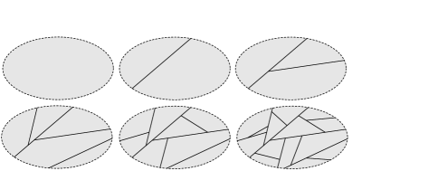
Figure 1: Construction of a STIT tessellation in a convex window with curved boundary.

Starting with [17], STIT tessellations and their theoretical framework were formally introduced in [18]. In [14, 15], a tessellation-valued random process on the positive real half-axis was constructed with the property that at each time the law of the tessellation is stable under iteration. This dynamic point of view also provides the link to a class of more general iteration infinitely divisible tessellations, which are in the focus of the present paper as well. In compact and convex windows $W\subset{\mathbb{R}}^{d}$ with positive volume, this process can be explained as follows. A terminal time $t>0$ and a (in some sense nondegenerate) measure $\Lambda$ on the space of hyperplanes in ${\mathbb{R}}^{d}$ are fixed in advance. Now $W$ is assigned a random lifetime. Upon expiry of its lifetime, $W$ dies and splits into two random sets separated by a hyperplane hitting $W$, which is chosen according to the suitable normalization of $\Lambda$. The resulting new random sets are again assigned independent random lifetimes and the entire construction continues recursively until the deterministic time threshold $t$ is reached, see Figure 1 for an illustration. The resulting random structure tessellates the window $W$ and is denoted by $Y(t\Lambda,W)$. In order to ensure the Markov property of this construction in the continuous-time parameter $t$ and in order to keep the law of $Y(t\Lambda,W)$ infinitely divisible or stable with respect to iterations, we will have to take care of the special choice of the lifetime distributions and the the cell-dividing hyperplanes, see Section 3 below. We would like to emphasize that the dynamical representation is a special feature of STIT tessellations and their infinitely divisible counterparts and, as recently pointed out in [21], that such and similar spatio-temporal random processes have remarkable potential for applications in stochastic geometry.

The purpose of the present paper is to explore the dynamic representation further and to introduce a new technique, which unifies and generalizes former approaches and which, moreover, has the advantage that it allows to deal with properties of the model that were out of reach so far. The crucial fact is that the construction above has an interpretation as a piecewise deterministic Markov process (PDMP) on the space of tessellations of $W$, which paves the way to the general theory of PDMP’s for which we refer to [6] in particular. This in turn puts us into the position to construct certain martingales related to the tessellation (see Section 4), eventually leading to fundamental comparison results of the tessellations under consideration with certain mixtures of Poisson hyperplane tessellations in Section 5. We would like to remark at this point that the theory of PDMP’s has previously successfully been applied in stochastic geometry and spatial statistics for the modeling of crack-growth networks, cf. [3, 4]. As applications of our comparison results we calculate in Section 6 several new mean values and also some new distributions related to geometric objects determined by the tessellation. To keep the paper self-contained, we recall in Section 2 the construction of STIT tessellations as limit of repeated iterations and formally introduce in Section 3 their Markovian dynamic representation. Moreover, we introduce there the above mentioned class of iteration infinitely divisible random tessellations and summarize some of their properties needed in this paper.

The current work is based on an extended version available online [22]. It also forms the basis of our papers [23, 24, 26, 25].

2 STIT tessellations as limits

Before explaining the concept of iteration of tessellations, let us fix some basic notions and notation. A tessellation of ${\mathbb{R}}^{d}$ is a locally finite partition of the space into compact convex polytopes, the cells of the tessellation. One can regard a tessellation either as a collection of its cells or as the closed set formed by the union of their boundaries. We will follow the second point of view and denote by $\operatorname{Cells}(Y)$ the set of cells of a tessellation $Y$. Thus, a random tessellation can be regarded as a special random closed set in the classical sense of stochastic geometry, see [20]. In particular, this imposes the usual Fell topology and the corresponding Borel measurable structure on the family of tessellations, see ibidem. By $\mathcal{K}_{d}$, we denote in this paper the space of compact and convex set in ${\mathbb{R}}^{d}$ with positive volume.

A random tessellation $Y$ is stationary if its distribution does not change upon actions of translations. Analogously a random tessellation is said to be isotropic if its distribution is invariant under the action of the rotation group $\mathit{SO}_{d}$.

Whenever two random tessellations $Y_{1}$ and $Y_{2}$ of ${\mathbb{R}}^{d}$ are given, we can define their iteration/nesting. For this purpose, we associate to each cell $c\in\operatorname{Cells}(Y_{1})$ an independent copy $Y_{2}(c)$ of $Y_{2}$ and we assume furthermore the family $\{Y_{2}(c)\colon\ c\in\operatorname{Cells}(Y_{1})\}$ to be independent of $Y_{1}$. Then we define the iteration of $Y_{1}$ with $Y_{2}$ by

$$Y_{1}\boxplus Y_{2}:=Y_{1}\cup\bigcup_{c\in\operatorname{Cells}(Y_{1})}\bigl{(}Y_{2}(c)\cap c\bigr{)},$$

that is, we take the local superposition of $Y_{1}$ and the family $\{Y_{2}(c)\colon\ c\in\operatorname{Cells}(Y_{1})\}$ inside the cells of $Y_{1}$. It was shown in [15] that with $Y_{1}$ and $Y_{2}$ also $Y_{1}\boxplus Y_{2}$ is a stationary random tessellation. A stationary random tessellation $Y$ is called stable under iterations, or STIT for short, if

$$m(\underbrace{Y\boxplus\cdots\boxplus Y}_{m\ \mathrm{times}})\stackrel{{\scriptstyle D}}{{=}}Y,\qquad m=2,3,\ldots,$$ (1)

where $\stackrel{{\scriptstyle D}}{{=}}$ stands for equality in distribution (note that rescaling with factor $m$ ensures that the mean surface area of cell boundaries per unit volume remains constant). In fact, using the uniqueness results Theorem 3 and Corollary 2 in [18] it is easy to see that it is enough to take one fixed $m>1$ in (1).

To proceed, let us be given a constant $0<t<\infty$ and an even (symmetric) probability measure $\mathcal{R}$ on the unit sphere ${\mathbb{S}}^{d-1}$, usually identified with the induced distribution of orthogonal hyperplanes on the space of $(d-1)$-dimensional linear hyperplanes in ${\mathbb{R}}^{d}$, also denoted by $\mathcal{R}$ in the sequel for notational simplicity. Define the measure $\Lambda$ on the space $\mathcal{H}$ of affine hyperplanes in ${\mathbb{R}}^{d}$ by

$$\Lambda:=\ell_{+}\otimes\mathcal{R},$$ (2)

with $\ell_{+}$ standing for the Lebesgue measure on the positive real half-axis $(0,\infty)$. Throughout this paper, we always require that the support of $\mathcal{R}$ spans the whole space. Assume now that we are given a stationary random tessellation $Y$ with surface intensity $t$ (i.e., the mean surface area of cell boundaries per unit volume equals $t$) and directional distribution $\mathcal{R}$ (i.e., the distribution of the normal direction of the facet containing the typical point is given by $\mathcal{R}$) and define the sequence $(\mathcal{I}_{n}(Y))_{n\geq 1}$ by

$$\mathcal{I}_{1}(Y):=2(Y\boxplus Y),\qquad\mathcal{I}_{n}(Y):=\frac{n}{n-1}\mathcal{I}_{n-1}(Y)\boxplus nY=n(\underbrace{Y\boxplus\cdots\boxplus Y}_{n\ \mathrm{times}}),\qquad n\geq 2.$$

It was shown in [18], Theorem 3, that $\mathcal{I}_{n}(Y)$ converges in law, as $n\to\infty$, to a stationary random limit tessellation $Y(t\Lambda)$ uniquely determined by $t\Lambda$. This tessellation is easily shown to be stable under iterations, whence a STIT tessellation with parameter $t$ and hyperplane measure $\Lambda$; we refer to Figure 2 for an illustration of the limit tessellation.

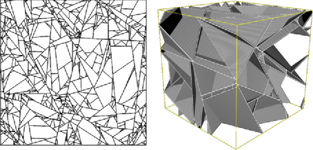
Figure 2: Realizations of a planar and a spatial stationary and isotropic STIT tessellation in a square and a cube, respectively.

3 The Markovian construction

As already emphasized in the Introduction, it is a crucial feature of the random tessellations $Y(t\Lambda)$ introduced in the previous section that they admit a simple and intuitive spatio-temporal Markovian construction. For a restriction $Y(t\Lambda,W)$ of $Y(t\Lambda)$ to a window $W\in\mathcal{K}_{d}$, this construction can be described as follows (the reader is referred to [18] for full details). Assign to $W$ an exponentially distributed random lifetime with parameter $\Lambda([W])$ where $[W]:=\{H\in\mathcal{H}\colon\ H\cap W\neq\varnothing\}$ stands for the family of all hyperplanes hitting $W$. Upon expiry of its lifetime, $W$ dies and splits into $W^{\pm}=W\cap H^{\pm}$ ($H^{\pm}$ are the two half-spaces determined by $H$), which are separated by a hyperplane in $[W]$ chosen according to the law $\Lambda(\cdot\cap[W])/\Lambda([W])$. The resulting new random sets $W^{+}$ and $W^{-}$ are again assigned independent exponential lifetimes with respective parameters $\Lambda([W^{+}])$ and $\Lambda([W^{-}])$ and the entire construction continues recursively until the deterministic time threshold $t$ is reached, see Figure 1. The separating $(d-1)$-dimensional facets (the word facet stands for a $(d-1)$-dimensional face here and throughout) arising in subsequent splits are usually referred to as $(d-1)$-dimensional maximal polytopes or I-segments for $d=2$ as assuming shapes similar to the letter I. (Note, that due to a possibly curved boundary of $W$ some of the maximal polytopes may also have a curved boundary and are no polytopes in the usual sense. However, we abuse notation and include also these sets in our class of maximal polytopes, which causes no difficulties in our theory.) The resulting random closed set constructed inside $W$ is denoted by $Y(t\Lambda,W)$, whereas the collection of all $(d-1)$-dimensional maximal polytopes or I-segments is denoted by $\operatorname{MaxPolytopes}_{d-1}(Y(t\Lambda,W))$. Moreover, we write $\operatorname{MaxPolytopes}_{k}(Y(t\Lambda,W))$ for the collection of $k$-dimensional maximal polytopes of $Y(t\Lambda,W)$, where a $k$-dimensional maximal polytope is just a $k$-dimensional face of some $(d-1)$-dimensional maximal polytope (again, some of them are no polytopes in the usual sense).

It was shown in [18] that the law of $Y(t\Lambda,W)$ is consistent in that $Y(t\Lambda,W)\cap V\stackrel{{\scriptstyle D}}{{=}}Y(t\Lambda,V)$ for convex $V\subset W$ and thus $Y(t\Lambda,W)$ can be extended to a random tessellation $Y(t\Lambda)$ in the whole space, which is then proved (see [18]) to coincide with the limit tessellation $Y(t\Lambda)$ considered in the previous section as notation already suggests. Again, the family of all $k$-dimensional maximal polytopes of $Y(t\Lambda)$ is denoted by $\operatorname{MaxPolytopes}_{k}(Y(t\Lambda))$ ($0\leq k\leq d-1$). The stationary random tessellation $Y(t\Lambda)$ is additionally isotropic if and only if $\mathcal{R}$ is the uniform distribution on ${\mathbb{S}}^{d-1}$ in the factorization (2).

A simple yet crucial observation is that even though only translation-invariant measures $\Lambda$ of the form (2) show up in the limiting STIT tessellations, the dynamic construction can be carried out with arbitrary non-atomic and locally finite measures $\Lambda$ on $\mathcal{H}$ also leading to a consistent family $Y(t\Lambda,W)$ and eventually, by extension, yielding a whole space tessellation $Y(t\Lambda)$. Many of our theorems will be stated in this general context. It should be emphasized that such tessellations are no longer iteration stable (STIT). However, they have the general property of being iteration infinitely divisible, as they can be readily checked to arise as $m$-fold iterations of $Y(t/m)$ for each $m\geq 2$ in all finite windows. Formally, this means that

$$Y\bigl{(}(t/m)\Lambda,W\bigr{)}^{\boxplus m}\stackrel{{\scriptstyle D}}{{=}}Y(t\Lambda,W)$$

for all $W\in\mathcal{K}_{d}$, which follows directly by construction as yielding

$$Y(s\Lambda,W)\boxplus Y(u\Lambda,W)\stackrel{{\scriptstyle D}}{{=}}Y\bigl{(}(s+u)\Lambda,W\bigr{)}.$$

It is worth pointing out that it is currently an open problem whether any iteration infinitely divisible random tessellation in ${\mathbb{R}}^{d}$ can be constructed in this way.

4 Associated martingales

The finite volume continuous-time incremental Markovian construction of iteration infinitely divisible random tessellations, or more specially of stationary STIT tessellations, as discussed in Sections 2 and 3 above, clearly enjoys the Markov property in the continuous time parameter. Whence, natural martingales arise, which will be of crucial importance for our further considerations. To discuss these processes, we notice that for any $W\in\mathcal{K}_{d}$ and any nonatomic locally finite hyperplane measure $\Lambda$, $(Y(t\Lambda,W))_{t>0}$ is a piecewise deterministic Markov process (PDMP) on the space of tessellations of $W$ and we cite Chapter 3 in [5], Chapter 7 in [6] and Chapter 12 in [7] for the general theory of such processes. Using these general results, we conclude that the PDMP $(Y(t\Lambda,W))_{t>0}$ has its infinitesimal generator ${\mathbb{L}}:={\mathbb{L}}_{\Lambda;W}$ given by

$${\mathbb{L}}F(Y)=\int_{[W]}\sum_{f\in\operatorname{Cells}(Y\cap H)}[F(Y\cup\{f\})-F(Y)]\Lambda(\mathrm{d}H),$$ (3)

where $Y$ is some instant of $Y(t\Lambda,W)$ and $F$ is some bounded measurable function on space of tessellations of $W$, cf. Theorem 12.22 in [7] in particular. Notice that for a tessellation $Y$ of $W\in\mathcal{K}_{d}$ and $H\in[W]$, $\operatorname{Cells}(Y\cap H)$ stands for the collection of $(d-1)$-dimensional cell of the sectional tessellation $Y\cap H$. By standard theory as given in Lemma 5.1, Appendix 1, Section 5 in [10] or, alternatively, by a direct check we readily conclude now.

Proposition 1

For $F$ bounded and measurable, the stochastic process

$$F(Y(t\Lambda,W))-\int_{0}^{t}{\mathbb{L}}F(Y(s\Lambda,W))\,\mathrm{d}s,\qquad t\geq 0,$$

is a martingale with respect to the filtration $\Im_{t}:=\sigma(Y(s\Lambda,W)\colon\ 0\leq s\leq t)$.

To proceed towards the crucial Proposition 2, consider $F$ of the form

$$\Sigma_{\phi}(Y):=\sum_{f\in\operatorname{MaxPolytopes}_{d-1}(Y)}\phi(f),$$ (4)

where $\phi(\cdot)$ is a generic bounded and measurable functional on $(d-1)$-dimensional facets in $W$, that is to say a bounded and measurable function on the space of closed $(d-1)$-dimensional polytopes in $W$, possibly chopped off by the boundary of $W$, with the standard measurable structure inherited from space of closed sets in $W$.

Proposition 2

The stochastic process

$$\Sigma_{\phi}(Y(t\Lambda,W))-\int_{0}^{t}\int_{[W]}\sum_{f\in\operatorname{Cells}(Y(s\Lambda,W)\cap H)}\phi(f)\Lambda(\mathrm{d}H)\,\mathrm{d}s,\qquad t\geq 0,$$

is a martingale with respect to $\Im_{t}$.

Proof.

The functional $\Sigma_{\phi}$ defined by (4) is not necessarily bounded and thus Proposition 1 cannot be applied directly with $F=\Sigma_{\phi}$ there. However, we can apply it for the truncations $\Sigma_{\phi}^{N}:=(\Sigma_{\phi}\wedge N)\vee-N,N\in{\mathbb{N}}$ and let $N\to\infty$ to conclude that

$$\Sigma_{\phi}(Y(t\Lambda,W))-\int_{0}^{t}{\mathbb{L}}\Sigma_{\phi}(Y(s\Lambda,W))\,\mathrm{d}s,\qquad t\geq 0$$

is a local $\Im_{t}$-martingale with a localizing sequence given by

$$\{\tau_{N}\}_{N\in{\mathbb{N}}}\qquad\mbox{with}\qquad\tau_{N}=\inf\{{t\geq 0}\colon\ |\Sigma_{\phi}(Y(t\Lambda,W))|\geq N\}.$$

Now, we apply the proof of Lemma 1 in [18], where the number of cells in $Y(t\Lambda,W)$, and hence for all $Y(s\Lambda,W),s\leq t$, has been shown to be bounded by a Furry–Yule-type linear birth process whose cardinality at any given finite time admits moments of all orders, to conclude that

$$\Sigma_{\phi}(Y(t\Lambda,W))-\int_{0}^{t}{\mathbb{L}}\Sigma_{\phi}(Y(s\Lambda,W))\,\mathrm{d}s,\qquad t\leq T,$$

is of class DL for all $T>0$ in the sense of Definition 4.8 in [8]. Using now the result of Problem 5.19(i) ibidem, we finally conclude that the random process

$$\Sigma_{\phi}(Y(t\Lambda,W))-\int_{0}^{t}{\mathbb{L}}\Sigma_{\phi}(Y(s\Lambda,W))\,\mathrm{d}s,\qquad t\geq 0,$$

is a martingale with respect to $\Im_{t}$. Moreover, in view of (3) we have

$${\mathbb{L}}\Sigma_{\phi}(Y) = \int_{[W]}\sum_{f\in\operatorname{Cells}(Y\cap H)}[\Sigma_{\phi}(Y\cup\{f\})-\Sigma_{\phi}(Y)]\Lambda(\mathrm{d}H)$$

$$= \int_{[W]}\sum_{f\in\operatorname{Cells}(Y\cap H)}\phi(f)\Lambda(\mathrm{d}H),$$

which completes the proof. ∎

5 Relationships for intensity measures

In this section, we establish two fundamental first-order properties of $Y(t\Lambda,W)$ for general locally finite nonatomic measures $\Lambda$, essentially obtained by comparison with suitable mixtures of Poisson hyperplane tessellations. The results are somehow surprising as formal identities and we are not able to provide an intuitive understanding. However, their applications in Corollary 1 and in Section 6 below have a very natural meaning and interpretation.

The key to our results is Proposition 2 from the previous section. To exploit it, consider the random measure

$$\mathcal{M}^{Y(t\Lambda,W)}:=\sum_{c\in\operatorname{Cells}(Y(t\Lambda,W))}\delta_{c}\quad\mbox{and}\quad{\mathbb{M}}^{Y(t\Lambda,W)}:={\mathbb{E}}\mathcal{M}^{Y(t\Lambda,W)}$$ (5)

with $\delta_{c}$ standing for the unit mass Dirac measure at $c$. In full analogy, define $\mathcal{M}^{\operatorname{PHT}(t\Lambda,W)}$ and ${\mathbb{M}}^{\operatorname{PHT}(t\Lambda,W)}$, where $\operatorname{PHT}(t\Lambda,W)$ is the Poisson hyperplane tessellation with intensity measure $t\Lambda$, restricted to $W$ (see [20] for background material). Further, put

$$\mathcal{F}_{k}^{Y(t\Lambda,W)}:=\sum_{f\in\operatorname{MaxPolytopes}_{k}(Y(t\Lambda,W))}\delta_{f},\qquad{\mathbb{F}}_{k}^{Y(t\Lambda,W)}:={\mathbb{E}}\mathcal{F}_{k}^{Y(t\Lambda,W)},\quad k=1,\ldots,d-1,$$

where, recall, $\operatorname{MaxPolytopes}_{k}(Y)$ is the collection of $k$-dimensional maximal polytopes of $Y$. Likewise, define

$$\mathcal{F}_{k}^{\operatorname{PHT}(t\Lambda,W)}:=\sum_{f\in\operatorname{Faces}_{k}(\operatorname{PHT}(t\Lambda,W))}\!\delta_{f},\qquad{\mathbb{F}}_{k}^{\operatorname{PHT}(t\Lambda,W)}:={\mathbb{E}}\mathcal{F}_{k}^{\operatorname{PHT}(t\Lambda,W)},\quad k=1,\ldots,d-1,$$

where $\operatorname{Faces}_{k}(\operatorname{PHT}(t\Lambda,W))$ is the collection of all $k$-face of the Poisson hyperplane tessellation $\operatorname{PHT}(t\Lambda,W)$. Our first claim is

Theorem 1

It holds that ${\mathbb{M}}^{Y(t\Lambda,W)}={\mathbb{M}}^{\operatorname{PHT}(t\Lambda,W)}$.

Proof.

Using (3) and (1) with

$$F(Y):=\sum_{c\in\operatorname{Cells}(Y)}\phi(c)$$

for a general bounded measurable cell functional $\phi$, with a localization argument as the one in the proof of Proposition 2 we conclude that

$$\int\phi(c^{\prime})\mathcal{M}^{Y(t\Lambda,W)}(\mathrm{d}c^{\prime})$$

$$\quad{}-\int_{0}^{t}\int_{[W]}\sum_{f\in\operatorname{Cells}(Y(s\Lambda,W)\cap H)}[\phi(\operatorname{Cell}^{+}(f,H|Y(s\Lambda,W)))+\phi(\operatorname{Cell}^{-}(f,H|Y(s\Lambda,W)))$$ (6)

$$\hphantom{\quad{}-\int_{0}^{t}\int_{[W]}\sum_{f\in\operatorname{Cells}(Y(s\Lambda,W)\cap H)}[}{}-\phi(\operatorname{Cell}(f,H|Y(s\Lambda,W)))]\Lambda(\mathrm{d}H)\,\mathrm{d}s,\qquad t\geq 0,$$

is a $\Im_{t}$-martingale. Here, $\operatorname{Cell}(f,H|Y(s\Lambda,W))$ stands for the a.s. uniquely determined cell of $Y(s\Lambda,W)$ that gets divided into $\operatorname{Cell}^{\pm}(f,H|Y(s\Lambda,W))$ by the facet $f$ on the hyperplane $H\in[W]$. To simplify the notation, we use $c^{\pm}(H)$ to denote the cells into which $c$ gets divided by $H$, lying, respectively, in the positive and negative half-space determined by $H$. With this notation, (5) says that

$$\int\phi(c^{\prime})\mathcal{M}^{Y(t\Lambda,W)}(\mathrm{d}c^{\prime})$$

$$\quad{}-\int_{0}^{t}\int\int_{[c]}[\phi(c^{+}(H))+\phi(c^{-}(H))-\phi(c)]\Lambda(\mathrm{d}H)\mathcal{M}^{Y(s\Lambda,W)}(\mathrm{d}c)\,\mathrm{d}s,\qquad t\geq 0$$

is a $\Im_{t}$-martingale. Taking expectations leads to

$$\int\phi(c^{\prime}){\mathbb{M}}^{Y(t\Lambda,W)}(\mathrm{d}c^{\prime})$$

(7)

$$\quad=\int_{0}^{t}\int\int_{[c]}[\phi(c^{+}(H))+\phi(c^{-}(H))-\phi(c)]\Lambda(\mathrm{d}H){\mathbb{M}}^{Y(s\Lambda,W)}(\mathrm{d}c)\,\mathrm{d}s$$

for all bounded measurable $\phi$ as above.

To proceed, we regard ${\mathbb{M}}^{Y(s\Lambda,W)}$ as an element of the space of bounded variation Borel measures on the family of polyhedral sub-cells of $W$ endowed with the standard measurable structure inherited from the space of closed sets in $W$. Consider the linear operator $T_{\Lambda}$ on this measure space given by

$$T_{\Lambda}\mu=\int\int_{[c]}[\delta_{c^{+}(H)}+\delta_{c^{-}(H)}-\delta_{c}]\Lambda(\mathrm{d}H)\mu(\mathrm{d}c).$$ (8)

By (8), $\|T_{\Lambda}\mu\|_{\mathrm{TV}}\leq(\int_{[W]}\mathrm{d}\Lambda)\|\mu\|_{\mathrm{TV}}=\Lambda([W])\|\mu\|_{\mathrm{TV}}$ where $\|\cdot\|_{\mathrm{TV}}$ is the standard total variation norm of a measure. This inequality turns into equality when $\mu=\delta_{W}$. Consequently, $T_{\Lambda}$ is a bounded operator of operator norm $\Lambda([W])<+\infty$ by the assumed locally finiteness of $\Lambda$. Using the operator $T_{\Lambda}$, relation (5) can be rewritten in form of an initial value problem for the operator differential equation

$$\frac{\partial}{\partial t}{\mathbb{M}}^{Y(t\Lambda,W)}=T_{\Lambda}{\mathbb{M}}^{Y(t\Lambda,W)},\qquad{\mathbb{M}}^{Y(0,W)}=\delta_{W},$$ (9)

which, in view of the above properties of $T_{\Lambda}$, admits by standard theory of linear operators (cf. [9], Chapter IX.§2, Section 2) the unique solution

$${\mathbb{M}}^{Y(t\Lambda,W)}=\exp(tT_{\Lambda})\delta_{W},\qquad t\geq 0,$$ (10)

where the operator exponential of $tT_{\lambda}$ is applied to the measure $\delta_{W}$. It is easily seen that exactly the same equations (5), (9) and thus also (10) hold for ${\mathbb{M}}^{\operatorname{PHT}(t\Lambda,W)}$. In particular, we have ${\mathbb{M}}^{Y(t\Lambda,W)}={\mathbb{M}}^{\operatorname{PHT}(t\Lambda,W)}$, as required. ∎

It is interesting to note that in the translation-invariant set-up, we obtain as a corollary that the distribution ${\mathbb{Q}}$ of the typical cell of the STIT tessellation $Y(t\Lambda)$ coincides with the typical cell distribution ${\mathbb{Q}}^{\operatorname{PHT}(t\Lambda)}$ of a stationary Poisson hyperplane tessellation $\operatorname{PHT}(t\Lambda)$ with intensity measure $t\Lambda$, a result that has previously been shown in [17] by completely different arguments. Recall, that – in intuitive terms – the typical cell of a tessellation is a randomly selected cell, where each cell has the same chance of being selected.

Corollary 1

In the translation-invariant set-up as considered in the previous paragraph it holds that $\mathbb{Q}={\mathbb{Q}}^{\operatorname{PHT}(t\Lambda)}$.

Proof.

The distribution ${\mathbb{Q}}$ is formally defined by the relation

$$\lambda_{d}{\mathbb{Q}}(A)=\lim_{r\rightarrow\infty}{{\mathbb{E}}\sum_{c\in\operatorname{Cells}(Y(t\Lambda))}\bm{1}[c\subset rW]\bm{1}[c-m(c)\in A]\over r^{d}\mathrm{V}_{d}(W)},$$ (11)

where $A$ is a measurable subset in the space of $d$-dimensional polytopes, $\lambda_{d}$ is the cell density of $Y(t\Lambda)$, $W\in\mathcal{K}_{d}$ and where $m(c)$ stands for some translation-covariant selector of the $d$-dimensional polytope $c$ (for example the Steiner point or the center of gravity), cf. [20], equation (4.8, 4.9). The distribution ${\mathbb{Q}}^{\operatorname{PHT}(t\Lambda)}$ is defined in a similar spirit. Here and below $\bm{1}[\cdot]$ stands for the usual indicator function, which is $1$ if the statement in brackets if fulfilled and $0$ otherwise. Rewriting the sum in (11) as an integral and using Campbell’s theorem, we obtain

$${\mathbb{E}}\sum_{c\in\operatorname{Cells}(Y(t\Lambda))}\bm{1}[c\subset rW]\bm{1}[c-m(c)\in A]$$

$$\quad=\int\bm{1}[c\subset rW]\bm{1}[c-m(c)\in A]{\mathbb{M}}^{Y(t\Lambda,rW)}(\mathrm{d}c),$$

where the condition $c\subset rW$ excludes from $Y(t\Lambda,rW)\stackrel{{\scriptstyle D}}{{=}}Y(t\Lambda)\cap rW$ those cells that hit the boundary of $rW$. Theorem 1 allows now to replace ${\mathbb{M}}^{Y(t\Lambda,rW)}$ by ${\mathbb{M}}^{\operatorname{PHT}(t\Lambda,rW)}$. Moreover, Theorem 1 clearly implies that the tessellations $Y(t\Lambda)$ and $\operatorname{PHT}(t\Lambda)$ have the same cell density, which in view of (11) completes the argument. ∎

Having characterized ${\mathbb{M}}^{Y(t\Lambda,W)}$, we now turn to the lower-dimensional face intensity measures ${\mathbb{F}}_{k}^{Y(t\Lambda,W)}$ in our general set-up, not necessarily assuming the translation-invariance of the hyperplane measure $\Lambda$.

Theorem 2

For all $k=0,\ldots,d-1$, it holds that

$${\mathbb{F}}_{k}^{Y(t\Lambda,W)}=(d-k)2^{d-k-1}\int_{0}^{t}\frac{1}{s}{\mathbb{F}}_{k}^{\operatorname{PHT}(s\Lambda,W)}\,\mathrm{d}s.$$

Proof.

Fix $k\in\{0,\ldots,d-1\}$. Let $\psi$ be a general bounded measurable function of a $k$-dimensional maximal polytope, as usual regarded as a closed subset of $W$, and for a $(d-1)$-dimensional maximal polytope $h$ put

$$\phi(h):=\sum_{f\in\operatorname{Faces}_{k}(h)}\psi(f),$$ (12)

noting that the $k$-dimensional maximal polytopes of the tessellation $Y(t\Lambda,W)$ are precisely the $k$-faces of its $(d-1)$-dimensional maximal polytopes. Using Proposition 2, taking expectations and recalling (5) we see that

$${\mathbb{E}}\Sigma_{\phi}(Y(t\Lambda,W))=\int\phi\,\mathrm{d}{\mathbb{F}}_{d-1}^{Y(t\Lambda,W)}=\int_{0}^{t}\int\int_{[c]}\phi(c\cap H)\Lambda(\mathrm{d}H){\mathbb{M}}^{Y(s\Lambda,W)}(\mathrm{d}c)\,\mathrm{d}s.$$

Applying Theorem 1, we get

$$\int\phi\,\mathrm{d}{\mathbb{F}}_{d-1}^{Y(t\Lambda,W)}=\int_{0}^{t}\int\int_{[c]}\phi(c\cap H)\Lambda(\mathrm{d}H){\mathbb{M}}^{\operatorname{PHT}(s\Lambda,W)}(\mathrm{d}c)\,\mathrm{d}s.$$ (13)

Now the Slivnyak–Mecke formula [20], Theorem 3.2.5 implies

$$\int\int_{[c]}\phi(c\cap H)\Lambda(\mathrm{d}H){\mathbb{M}}^{\operatorname{PHT}(\Lambda,W)}(\mathrm{d}c)=\int\phi\,\mathrm{d}{\mathbb{F}}_{d-1}^{\operatorname{PHT}(\Lambda,W)}.$$ (14)

Indeed, identifying $\operatorname{PHT}(\Lambda,W)$ with the collection of Poisson hyperplanes hitting $W$ we have

$$\int\phi\,\mathrm{d}{\mathbb{F}}_{d-1}^{\operatorname{PHT}(\Lambda,W)}$$

$$\quad={\mathbb{E}}\sum_{H\in\operatorname{PHT}(\Lambda,W)}\sum_{f\in\operatorname{Cells}(\operatorname{PHT}(\Lambda,W)\cap H)}\phi(f)=\int_{[W]}{\mathbb{E}}\sum_{f\in\operatorname{Cells}(\operatorname{PHT}(\Lambda,W)\cap H)}\phi(f)\Lambda(\mathrm{d}H)$$

$$\quad={\mathbb{E}}\sum_{c\in\operatorname{Cells}(\operatorname{PHT}(\Lambda,W))}\int_{[c]}\phi(c\cap H)\Lambda(\mathrm{d}H)=\int\int_{[c]}\phi(c\cap H)\Lambda(\mathrm{d}H){\mathbb{M}}^{\operatorname{PHT}(\Lambda,W)}(\mathrm{d}c).$$

Taking in (14) now $s\Lambda$ in place of $\Lambda$ we find more generally

$$\int\int_{[c]}\phi(c\cap H)\Lambda(\mathrm{d}H){\mathbb{M}}^{\operatorname{PHT}(s\Lambda,W)}(\mathrm{d}c)=\frac{1}{s}\int\phi\,\mathrm{d}{\mathbb{F}}_{d-1}^{\operatorname{PHT}(s\Lambda,W)},$$

whence, with (13),

$$\int\phi\,\mathrm{d}{\mathbb{F}}_{d-1}^{Y(t\Lambda,W)}=\int_{0}^{t}\frac{1}{s}\int\phi\,\mathrm{d}{\mathbb{F}}_{d-1}^{\operatorname{PHT}(s\Lambda,W)}\,\mathrm{d}s.$$

We note now that, by (12),

$$\int\phi\,\mathrm{d}{\mathbb{F}}_{d-1}^{Y(t\Lambda,W)}=\int\psi\,\mathrm{d}{\mathbb{F}}_{k}^{Y(t\Lambda,W)},$$

because each $k$-dimensional maximal polytope is a $k$-face of precisely one $(d-1)$-dimensional maximal polytope in $Y(t\Lambda,W)$. On the other hand,

$$\int\phi\,\mathrm{d}{\mathbb{F}}_{d-1}^{\operatorname{PHT}(s\Lambda,W)}=(d-k)2^{d-k-1}\int\psi\,\mathrm{d}{\mathbb{F}}_{k}^{\operatorname{PHT}(s\Lambda,W)},$$

because each $k$-face of $\operatorname{PHT}(s\Lambda,W)$ is a $k$-face of $(d-k)2^{d-k-1}$ facets of $\operatorname{PHT}(s\Lambda,W)$, see Theorems 10.1.2 and 10.3.1 in [20]. Hence, we conclude that

$$\int\psi\,\mathrm{d}{\mathbb{F}}_{k}^{Y(t\Lambda,W)}=(d-k)2^{d-k-1}\int_{0}^{t}\frac{1}{s}\int\psi\,\mathrm{d}{\mathbb{F}}_{k}^{\operatorname{PHT}(s\Lambda,W)}\,\mathrm{d}s$$

for all $\psi$ bounded and measurable, which completes the proof of the theorem. ∎

Some of our arguments in the sequel and the theory developed in [23, 24], for example, require a straightforward formal extension of Theorem 2. Namely, we formally mark all $(d-1)$-dimensional maximal polytopes of the tessellation $Y(t\Lambda,W)$ by their birth times. This gives rise to the birth-time augmented tessellation $\hat{Y}(t,W)$ with birth-time-marked $(d-1)$-dimensional maximal polytopes and makes the Markovian construction of $\hat{Y}(t,W)$ into a Markov process whose generator $\hat{{\mathbb{L}}}$ is a clear modification of ${\mathbb{L}}$ as given in (3):

$$\hat{\mathbb{L}}\hat{F}(\hat{Y}(s,W))=\int_{[W]}\sum_{f\in\operatorname{Cells}(Y(s,W)\cap H)}\bigl{[}\hat{F}(\hat{Y}(s,W)\cup[\{f\},s])-\hat{F}(\hat{Y}(s,W))\bigr{]}\Lambda(\mathrm{d}H)$$

for $\hat{F}$ bounded and measurable on the space of birth-time-marked tessellations of $W$. Consequently, writing $\hat{\mathbb{F}}^{Y(t\Lambda,W)}_{k},k=0,\ldots,d-1$, for the birth-time-marked version of ${\mathbb{F}}^{Y(t\Lambda,W)}_{k}$, where each $k$-dimensional maximal polytope is marked with its birth time, by a straightforward modification of the proof of Theorem 2 we are led to the following.

Corollary 2

For all $k=0,\ldots,d-1$ it holds that

$$\hat{\mathbb{F}}^{Y(t\Lambda,W)}_{k}=(d-k)2^{d-k-1}\int_{0}^{t}\frac{1}{s}\bigl{[}{\mathbb{F}}^{\operatorname{PHT}(s\Lambda,W)}_{k}\otimes\delta_{s}\bigr{]}\,\mathrm{d}s.$$

6 Typical maximal polytope distributions

We are now going to apply the results obtained in the last section to the stationary set-up, that is, with $\Lambda$ translation-invariant, to study the distribution of typical $k$-dimensional maximal polytopes of the STIT tessellation $Y(t\Lambda)$ in ${\mathbb{R}}^{d}$. Recall, that, in intuitive terms, the typical $k$-dimensional maximal polytope of $Y(t\Lambda)$ is what we get when we equiprobably choose one of the tessellations $k$-dimensional maximal polytopes. The typical $k$-dimensional maximal polytope distribution ${\mathbb{Q}}_{k}$ ($1\leq k\leq d-1$) is formally given by

$$\lambda_{k}{\mathbb{Q}}_{k}(A)=\lim_{r\rightarrow\infty}{1\over\mathrm{V}_{d}(rW)}\sum_{f\in\operatorname{MaxPolytopes}_{k}(Y(t\Lambda))}\bm{1}[f\subset rW]\bm{1}[f-m(f)\in A],$$ (15)

where $\lambda_{k}$ is the mean number of $k$-dimensional maximal polytope selectors $m(f)$ of $Y(t\Lambda)$ per unit volume (this is the intensity of $\operatorname{MaxPolytopes}_{k}(Y(t\Lambda))$), $A$ is a measurable subset of the space of $k$-dimensional polytopes, $W\in\mathcal{K}_{d}$ and, as in the proof of Corollary 1, where $m(f)$ stands for some translation-covariant selector of $f$ (as its Steiner point for example). Similarly, the distribution ${\mathbb{Q}}_{k}^{\operatorname{PHT}(t\Lambda)}$ of the typical $k$-face of a Poisson hyperplane tessellation with intensity measure $t\Lambda$ is defined, see Chapter 4.1 in [20].

Theorem 3

For $k\in\{1,\ldots,d-1\}$, the distribution ${\mathbb{Q}}_{k}$ of the typical $k$-dimensional maximal polytope of $Y(t\Lambda)$ is given by

$${\mathbb{Q}}_{k}=\int_{0}^{t}{{d}s^{d-1}\over t^{d}}{\mathbb{Q}}_{k}^{\operatorname{PHT}(s\Lambda)}\,\mathrm{d}s.$$

The preceding theorem can be rephrased by saying that the distribution of the typical $k$-dimensional maximal polytope of a STIT tessellation is a mixture of suitable rescalings of distributions of typical $k$-dimensional faces of Poisson hyperplane tessellations, and that the mixing distribution is a beta-distribution on $(0,t)$ with parameters $d$ and $1$, which has density ${\,\mathrm{d}s^{d-1}\over t^{d}}\bm{1}[0<s<t]$. Proof of Theorem 3 To start, let $\varphi_{k}$ be a real-valued, bounded, translation-invariant, non-negative measurable function on the space of $k$-dimensional polytopes ($1\leq k\leq d-1$) and denote by $\overline{\varphi}_{k}(Y(t\Lambda))$ the (possibly infinite) $\varphi_{k}$-density of $Y(t\Lambda)$ in the sense of [20], Chapter 4.1, that is,

$$\overline{\varphi}_{k}(Y(t\Lambda))=\lim_{r\rightarrow\infty}{1\over\mathrm{V}_{d}(rW)}{\mathbb{E}}\sum_{f\in\operatorname{MaxPolytopes}_{k}(Y(t\Lambda))}\bm{1}[f\subset rW]\varphi_{k}(f)$$ (16)

with $W\in\mathcal{K}_{d}$. The existence of this limit is guaranteed by Theorem 4.1.3 ibidem. Using now Campbell’s theorem [20], Theorem 3.1.2 and Theorem 2 from above, we obtain, possibly with both sides infinite,

$$\overline{\varphi}_{k}(Y(t\Lambda)) = \lim_{r\rightarrow\infty}{1\over\mathrm{V}_{d}(rW)}{\mathbb{E}}\sum_{f\in\operatorname{MaxPolytopes}_{k}(Y(t\Lambda))}\bm{1}[f\subset rW]\varphi_{k}(f)$$

$$= \lim_{r\rightarrow\infty}{1\over\mathrm{V}_{d}(rW)}{\mathbb{E}}\int\bm{1}[f\subset rW]\varphi_{k}(f)\mathcal{F}_{k}^{Y(t\Lambda,rW)}(\mathrm{d}f)$$

$$= \lim_{r\rightarrow\infty}{1\over\mathrm{V}_{d}(rW)}\int\bm{1}[f\subset rW]\varphi_{k}(f){\mathbb{F}}_{k}^{Y(t\Lambda,rW)}(\mathrm{d}f)$$

$$= \lim_{r\rightarrow\infty}{(d-k)2^{d-k-1}\over\mathrm{V}_{d}(rW)}\int_{0}^{t}{1\over s}\int\bm{1}[f\subset rW]\varphi_{k}(f){\mathbb{F}}_{k}^{\operatorname{PHT}(s\Lambda,rW)}(\mathrm{d}f)\,\mathrm{d}s.$$

By dominated convergence, we can continue as follows:

$$= (d-k)2^{d-k-1}\int_{0}^{t}{1\over s}\biggl{[}\lim_{r\rightarrow\infty}{1\over\mathrm{V}_{d}(rW)}{\mathbb{E}}\sum_{f\in\operatorname{Faces}_{k}(\operatorname{PHT}(s\Lambda))}\bm{1}[f\subset rW]\varphi_{k}(f)\biggr{]}\,\mathrm{d}s$$

$$= (d-k)2^{d-k-1}\int_{0}^{t}{1\over s}\overline{\varphi}_{k}(\operatorname{PHT}(s\Lambda))\,\mathrm{d}s.$$

For $\varphi_{k}\equiv 1$ we find $\lambda_{k}=\overline{\varphi}_{k}(Y(t\Lambda))$, which clearly has an interpretation as intensity of $k$-dimensional maximal polytopes. Similarly, we denote by $\lambda_{k}^{\operatorname{PHT}(s\Lambda)}$ the intensity of $k$-faces of the Poisson hyperplane tessellation $\operatorname{PHT}(s\Lambda)$ and notice that $s\operatorname{PHT}(s\Lambda)\stackrel{{\scriptstyle D}}{{=}}\operatorname{PHT}(\Lambda)$. Hence, there is a constant $C_{k}\in(0,\infty)$, which is independent of $s$, such that $\lambda_{k}^{\operatorname{PHT}(s\Lambda)}=C_{k}s^{d}$ (in fact $C_{k}$ is explicitly known and given by equation (10.44) in [20]). Thus, in view of (6) we get

$$\lambda_{k}=(d-k)2^{d-k-1}\int_{0}^{t}{1\over s}C_{k}s^{d}\,\mathrm{d}s={d-k\over d}2^{d-k-1}C_{k}t^{d}={d-k\over d}2^{d-k-1}\lambda_{k}^{\operatorname{PHT}(t\Lambda)}.$$ (18)

Let $m(f)$ with $f\in\operatorname{MaxPolytopes}_{k}(Y(t\Lambda))$ be as in (15). Using (6), this time with $\varphi_{k}(f):=\bm{1}[f-m(f)\in\cdot]$, together with (15), we obtain

$$\lambda_{k}{\mathbb{Q}}_{k}=(d-k)2^{d-k-1}\int_{0}^{t}{1\over s}\lambda_{k}^{\operatorname{PHT}(s\Lambda)}{\mathbb{Q}}_{k}^{\operatorname{PHT}(s\Lambda)}\,\mathrm{d}s.$$ (19)

Combining (19) with (18) we find, with $C_{k}$ as above,

$${\mathbb{Q}}_{k} = (d-k)2^{d-k-1}\int_{0}^{t}{1\over s}{\lambda_{k}^{\operatorname{PHT}(s\Lambda)}\over\lambda_{k}}{\mathbb{Q}}_{k}^{\operatorname{PHT}(s\Lambda)}\,\mathrm{d}s=\int_{0}^{t}{d\over s}{\lambda_{k}^{\operatorname{PHT}(s\Lambda)}\over\lambda_{k}^{\operatorname{PHT}(t\Lambda)}}{\mathbb{Q}}_{k}^{\operatorname{PHT}(s\Lambda)}\,\mathrm{d}s$$

$$= \int_{0}^{t}{d\over s}{C_{k}s^{d}\over C_{k}t^{d}}{\mathbb{Q}}_{k}^{\operatorname{PHT}(s\Lambda)}\,\mathrm{d}s=\int_{0}^{t}{{d}s^{d-1}\over t^{d}}{\mathbb{Q}}_{k}^{\operatorname{PHT}(s\Lambda)}\,\mathrm{d}s,$$

which is the desired expression for ${\mathbb{Q}}_{k}$.

It is interesting to note that formally marking the $k$-dimensional maximal polytopes with their birth-times and repeating the argument leading to Theorem 3 with Theorem 2 replaced by its time-marked extension in Corollary 2 we obtain the birth time-marked extension of Theorem 3:

Corollary 3

The distribution $\hat{\mathbb{Q}}_{k}$ of the typical birth-time-marked $k$-dimensional maximal polytope of $Y(t\Lambda)$ is given by

$$\hat{\mathbb{Q}}_{k}=\int_{0}^{t}{ds^{d-1}\over t^{d}}\bigl{[}{\mathbb{Q}}_{k}^{\operatorname{PHT}(s\Lambda)}\otimes\delta_{s}\bigr{]}\,\mathrm{d}s,$$

where $k\in\{1,\ldots,d-1\}$ as above.

From these identities, mean values and also distributional results for the typical $k$-dimensional maximal polytope of a stationary STIT tessellation can be deduced. To illustrate the general method, we exemplarily calculate at first the mean intrinsic volumes of the typical $k$-dimensional maximal polytope of the STIT tessellation $Y(t\Lambda)$. To neatly formulate them, let $\Pi$ be the associated zonoid of the Poisson hyperplane tessellation $\operatorname{PHT}(t\Lambda)$. This is the convex body which has its support $h_{\Pi}(u)$ function given by

$$h_{\Pi}(u)={t\over 2}\int_{{\mathbb{S}}^{d-1}}|\langle u,v\rangle|\mathcal{R}(\mathrm{d}v),\qquad u\in{\mathbb{R}}^{d},$$

see [20], equation (4.59), where $\langle\cdot,\cdot\rangle$ denotes the standard scalar product in ${\mathbb{R}}^{d}$. Moreover, we will denote by $V_{j}(K)$ the intrinsic volume of order $j$ of $K\in\mathcal{K}_{d}$ in the usual sense of integral geometry. In particular, $V_{d}(K)$ is the volume, $2V_{d-1}(K)$ the surface area, $V_{1}(K)$ a constant multiple of the mean width and $V_{0}(K)=1$ the Euler-characteristic of $K$, cf. [20].

Corollary 4

Fix $0\leq j\leq k\leq d-1$. The mean $j$th intrinsic volume $V_{j}$ of the typical $k$-dimensional maximal polytope $I_{k}$ (this is a random polytope with distribution ${\mathbb{Q}}_{k}$) is given by

$${\mathbb{E}}V_{j}(I_{k})={d\over d-j}{{d-j\choose d-k}\over{d\choose k}}{V_{d-k}(\Pi)\over\mathrm{V}_{d}(\Pi)}.$$

Proof.

Using Theorem 3, Theorem 10.3.3 in [20] and the homogeneity of the intrinsic volumes, we get

$${\mathbb{E}}V_{j}(I_{k}) = \int_{0}^{t}{ds^{d-1}\over t^{d}}{{d-j\choose d-k}V_{d-j}((s/t)\Pi)\over{d\choose k}\mathrm{V}_{d}((s/t)\Pi)}\,\mathrm{d}s={{d-j\choose d-k}\over{d\choose k}}{V_{d-k}(\Pi)\over\mathrm{V}_{d}(\Pi)}\int_{0}^{t}{ds^{d-1}\over t^{d}}{(s/t)^{d-j}\over(s/t)^{d}}\,\mathrm{d}s$$

$$= {d\over d-j}{{d-j\choose d-k}\over{d\choose k}}{V_{d-k}(\Pi)\over\mathrm{V}_{d}(\Pi)},$$

which completes the proof. ∎

Note that in the isotropic case, that is, when $\mathcal{R}$ is the uniform distribution on ${\mathbb{S}}^{d-1}$ in the factorization (2), the zonoid $\Pi$ is a $d$-dimensional ball with radius proportional to $t$. More specifically, we have in this case

$${\mathbb{E}}V_{j}(I_{k})={d\over d-j}{k\choose j}\biggl{(}{d\kappa_{d}\over\kappa_{d-1}}\biggr{)}^{j}{1\over\kappa_{j}t^{j}},$$

where $\kappa_{j}$ is the volume of the $j$-dimensional unit ball.

Remark 1.

In the planar ($d=2$) and in the spatial case ($d=3$), the mean values ${\mathbb{E}}V_{j}(I_{k})$ are in accordance with the values obtained earlier in [13, 19], for example. The method there was based on the stochastic stability of the tessellation under iterations, which leads to balance equations for ${\mathbb{E}}V_{j}(I_{k})$ that can be solved by using intersection formulae for random tessellations. It seems, however, that this method becomes impracticable in higher space dimensions.

Remark 2.

Corollary 4 shows that the intrinsic volumes $V_{j}$ ($0\leq j\leq k$) are integrable with respect to ${\mathbb{Q}}_{k}$ ($1\leq k\leq d-1$), the typical $k$-dimensional maximal polytope distribution. In view of Theorem 4.1.2 in [20] this allows us to replace the definition (16) of $\overline{\varphi}_{k}$ by

$$\overline{\varphi}_{k}(Y(t\Lambda)) = \lim_{r\rightarrow\infty}{1\over\mathrm{V}_{d}(rW)}{\mathbb{E}}\sum_{f\in\operatorname{MaxPolytopes}_{k}(Y(t\Lambda,rW))}\varphi_{k}(f)$$

$$= \lim_{r\rightarrow\infty}{1\over\mathrm{V}_{d}(rW)}\int\varphi_{k}(f){\mathbb{F}}_{k}^{Y(t\Lambda,rW)},$$

not excluding thereby those maximal polytopes hitting the boundary of $W\in\mathcal{K}_{d}$, which is somehow more natural in view of our setting in Section 5.

As a second example, we turn now to the length distribution of the typical I-segment, which is nothing than the typical maximal polytope of dimension one.

Corollary 5

The distribution of the length of the typical I-segment of a stationary and isotropic STIT tessellation with time parameter $t>0$ is a mixture of exponential distributions with parameter $\gamma s$. The mixing distribution is a beta-distribution on $(0,t)$ with parameters $d$ and $1$. Its density is given by

$$p_{d}(x)=\int_{0}^{t}\gamma s\mathrm{e}^{-\gamma sx}{ds^{d-1}\over t^{d}}\,\mathrm{d}s={d\over(\gamma t)^{d}x^{d+1}}\Gamma(d+1,\gamma tx),\qquad x>0,$$

where $\Gamma(\cdot,\cdot)$ is the lower incomplete Gamma-function and $\gamma=\Gamma(d/2)/(\Gamma(1/2)\Gamma((d+1)/2))$.

Proof.

This follows immediately from Theorem 3 and the well-known fact that the length distribution of the typical edge of a stationary and isotropic Poisson hyperplane tessellation with intensity $0<s<t$ is an exponential distribution with parameter $\gamma s$, see [1]. ∎

In particular for $d=2$ and $d=3$, we have the densities

$$p_{2}(x) = {1\over t^{2}x^{3}}\bigl{(}\uppi^{2}-(\uppi^{2}+2\uppi tx+2t^{2}x^{2})\mathrm{e}^{-(2/\uppi)tx}\bigr{)},\qquad x>0,$$

$$p_{3}(x) = {3\over t^{3}x^{4}}\bigl{(}48-(48+24tx+6t^{2}x^{2}+t^{3}x^{3})\mathrm{e}^{-(1/2)tx}\bigr{)},\qquad x>0.$$

The mean segment lengths are $\uppi/t$ in the planar case and $3/t$ for $d=3$. Moreover, the variance of the length of the typical I-segment in the spatial case is given by $24/t^{2}$, which was not available before. In general, from the explicit length density formula it is easily seen that for the length of the typical I-segment only the moments of order $1$ up to $d-1$ are finite.

Let us finally remark that Corollary 5 allows an extension to the anisotropic setting. Theorem 3 also implies that the conditional length distribution of the typical I-segment in $Y(t\Lambda)$ (where now $\Lambda$ is a general translation-invariant hyperplane measure as in (2)), given its birth time $s\in(0,1)$ and direction $u\in{\mathbb{S}}^{d-1}$, is an exponential distribution with parameter $s\Lambda([e(u)])$, where $e(u)$ is a line segment of unit length parallel to $u$. Thus, the conditional distribution of the length of the typical I-segment with a given direction is a mixture of these exponential distributions and the mixing distribution has again density ${ds^{d-1}\over t^{d}}\bm{1}[0<s<t]$.

Remark 3.

The length density $p_{2}(x)$ of the typical I-segment in a planar stationary and isotropic STIT tessellation has been calculated in [13] by an entirely different method based on Palm theory. However, this method seems to be restricted to the study of I-segments and does not lead to results for higher-dimensional maximal polytopes as in Theorem 3 above.

References

- [1] {barticle}[mr] \bauthor\bsnmBaumstark, \bfnmVolker\binitsV. &\bauthor\bsnmLast, \bfnmGünter\binitsG. (\byear2009). \btitleGamma distributions for stationary Poisson flat processes. \bjournalAdv. in Appl. Probab. \bvolume41 \bpages911–939. \biddoi=10.1239/aap/1261669578, issn=0001-8678, mr=2663228 \bptokimsref \endbibitem
- [2] {barticle}[mr] \bauthor\bsnmBeil, \bfnmMichael\binitsM., \bauthor\bsnmEckel, \bfnmStefanie\binitsS., \bauthor\bsnmFleischer, \bfnmFrank\binitsF., \bauthor\bsnmSchmidt, \bfnmHendrik\binitsH., \bauthor\bsnmSchmidt, \bfnmVolker\binitsV. &\bauthor\bsnmWalther, \bfnmPaul\binitsP. (\byear2006). \btitleFitting of random tessellation models to keratin filament networks. \bjournalJ. Theoret. Biol. \bvolume241 \bpages62–72. \biddoi=10.1016/j.jtbi.2005.11.009, issn=0022-5193, mr=2250184 \bptokimsref \endbibitem
- [3] {barticle}[pbm] \bauthor\bsnmBeil, \bfnmMichael\binitsM., \bauthor\bsnmLück, \bfnmSebastian\binitsS., \bauthor\bsnmFleischer, \bfnmFrank\binitsF., \bauthor\bsnmPortet, \bfnmStéphanie\binitsS., \bauthor\bsnmArendt, \bfnmWolfgang\binitsW. &\bauthor\bsnmSchmidt, \bfnmVolker\binitsV. (\byear2009). \btitleSimulating the formation of keratin filament networks by a piecewise-deterministic Markov process. \bjournalJ. Theor. Biol. \bvolume256 \bpages518–532. \biddoi=10.1016/j.jtbi.2008.09.044, issn=1095-8541, pii=S0022-5193(08)00504-3, pmid=19014958 \bptokimsref \endbibitem
- [4] {barticle}[mr] \bauthor\bsnmChiquet, \bfnmJulien\binitsJ., \bauthor\bsnmLimnios, \bfnmNikolaos\binitsN. &\bauthor\bsnmEid, \bfnmMohamed\binitsM. (\byear2009). \btitlePiecewise deterministic Markov processes applied to fatigue crack growth modelling. \bjournalJ. Statist. Plann. Inference \bvolume139 \bpages1657–1667. \biddoi=10.1016/j.jspi.2008.05.034, issn=0378-3758, mr=2494482 \bptokimsref \endbibitem
- [5] {bbook}[auto:STB—2012/03/21—07:41:58] \bauthor\bsnmGikhman, \bfnmIosif I.\binitsI.I. &\bauthor\bsnmSkorokhod, \bfnmAnatoli V.\binitsA.V. (\byear1974). \btitleThe Theory of Stochastic Processes. II. \baddressBerlin: \bpublisherSpringer. \bptnotecheck year \bptokimsref \endbibitem
- [6] {bbook}[mr] \bauthor\bsnmJacobsen, \bfnmMartin\binitsM. (\byear2006). \btitlePoint Process Theory and Applications: Marked Point and Piecewise Deterministic Processes. \bseriesProbability and Its Applications. \baddressBoston, MA: \bpublisherBirkhäuser. \bidmr=2189574 \bptokimsref \endbibitem
- [7] {bbook}[mr] \bauthor\bsnmKallenberg, \bfnmOlav\binitsO. (\byear2002). \btitleFoundations of Modern Probability, \bedition2nd ed. \bseriesProbability and Its Applications (New York). \baddressNew York: \bpublisherSpringer. \bidmr=1876169 \bptokimsref \endbibitem
- [8] {bbook}[auto:STB—2012/03/21—07:41:58] \bauthor\bsnmKaratzas, \bfnmIoannis\binitsI. &\bauthor\bsnmShreve, \bfnmSteven E.\binitsS.E. (\byear1998). \btitleBrownian Motion and Stochastic Calculus, \bedition2nd ed. \baddressNew York: \bpublisherSpringer. \bptnotecheck year \bptokimsref \endbibitem
- [9] {bbook}[auto:STB—2012/03/21—07:41:58] \bauthor\bsnmKato, \bfnmT.\binitsT. (\byear1966). \btitlePerturbation Theory for Linear Operators. \baddressBerlin: \bpublisherSpringer. \bptokimsref \endbibitem
- [10] {bbook}[mr] \bauthor\bsnmKipnis, \bfnmClaude\binitsC. &\bauthor\bsnmLandim, \bfnmClaudio\binitsC. (\byear1999). \btitleScaling Limits of Interacting Particle Systems. \bseriesGrundlehren der Mathematischen Wissenschaften [Fundamental Principles of Mathematical Sciences] \bvolume320. \baddressBerlin: \bpublisherSpringer. \bidmr=1707314 \bptokimsref \endbibitem
- [11] {barticle}[mr] \bauthor\bsnmLautensack, \bfnmClaudia\binitsC. (\byear2008). \btitleFitting three-dimensional Laguerre tessellations to foam structures. \bjournalJ. Appl. Stat. \bvolume35 \bpages985–995. \biddoi=10.1080/02664760802188112, issn=0266-4763, mr=2522123 \bptokimsref \endbibitem
- [12] {bincollection}[auto:STB—2012/03/21—07:41:58] \bauthor\bsnmLautensack, \bfnmC.\binitsC. &\bauthor\bsnmSych, \bfnmT.\binitsT. (\byear2005). \btitle3d image analysis of foams using random tessellations. In \bbooktitleProceedings of the 9th European Congress on Stereology and Image Analysis and 7th STERMAT International Conference on Stereology and Image Analysis in Materials Science in Zakopane \bpages147–153. \bptokimsref \endbibitem
- [13] {barticle}[auto] \bauthor\bsnmMecke, \bfnmJ.\binitsJ., \bauthor\bsnmNagel, \bfnmW.\binitsW. &\bauthor\bsnmWeiss, \bfnmV.\binitsV. (\byear2007). \btitleLength distributions of edges in planar stationary and isotropic STIT tessellations. \bjournalJ. Contemp. Math. Anal. \bvolume42 \bpages28–43. \bptokimsref \endbibitem
- [14] {barticle}[mr] \bauthor\bsnmMecke, \bfnmJ.\binitsJ., \bauthor\bsnmNagel, \bfnmW.\binitsW. &\bauthor\bsnmWeiss, \bfnmV.\binitsV. (\byear2008). \btitleA global construction of homogeneous random planar tessellations that are stable under iteration. \bjournalStochastics \bvolume80 \bpages51–67. \biddoi=10.1080/17442500701605403, issn=1744-2508, mr=2384821 \bptokimsref \endbibitem
- [15] {barticle}[mr] \bauthor\bsnmMecke, \bfnmJoseph\binitsJ., \bauthor\bsnmNagel, \bfnmWerner\binitsW. &\bauthor\bsnmWeiss, \bfnmViola\binitsV. (\byear2008). \btitleThe iteration of random tessellations and a construction of a homogeneous process of cell divisions. \bjournalAdv. in Appl. Probab. \bvolume40 \bpages49–59. \biddoi=10.1239/aap/1208358886, issn=0001-8678, mr=2411814 \bptokimsref \endbibitem
- [16] {barticle}[mr] \bauthor\bsnmNagel, \bfnmWerner\binitsW., \bauthor\bsnmMecke, \bfnmJoseph\binitsJ., \bauthor\bsnmOhser, \bfnmJoachim\binitsJ. &\bauthor\bsnmWeiss, \bfnmViola\binitsV. (\byear2008). \btitleA tessellation model for crack patterns on surfaces. \bjournalImage Anal. Stereol. \bvolume27 \bpages73–78. \biddoi=10.5566/ias.v27.p73-78, issn=1580-3139, mr=2455218 \bptokimsref \endbibitem
- [17] {barticle}[mr] \bauthor\bsnmNagel, \bfnmWerner\binitsW. &\bauthor\bsnmWeiss, \bfnmViola\binitsV. (\byear2003). \btitleLimits of sequences of stationary planar tessellations. \bjournalAdv. in Appl. Probab. \bvolume35 \bpages123–138. \bnoteIn honor of Joseph Mecke. \biddoi=10.1239/aap/1046366102, issn=0001-8678, mr=1975507 \bptokimsref \endbibitem
- [18] {barticle}[mr] \bauthor\bsnmNagel, \bfnmWerner\binitsW. &\bauthor\bsnmWeiss, \bfnmViola\binitsV. (\byear2005). \btitleCrack STIT tessellations: Characterization of stationary random tessellations stable with respect to iteration. \bjournalAdv. in Appl. Probab. \bvolume37 \bpages859–883. \biddoi=10.1239/aap/1134587744, issn=0001-8678, mr=2193987 \bptokimsref \endbibitem
- [19] {barticle}[auto:STB—2012/03/21—07:41:58] \bauthor\bsnmNagel, \bfnmW.\binitsW. &\bauthor\bsnmWeiss, \bfnmV.\binitsV. (\byear2008). \btitleMean values for homogeneous STIT tessellations in 3D. \bjournalImage Anal. Stereol. \bvolume27 \bpages29–37. \bptokimsref \endbibitem
- [20] {bbook}[mr] \bauthor\bsnmSchneider, \bfnmRolf\binitsR. &\bauthor\bsnmWeil, \bfnmWolfgang\binitsW. (\byear2008). \btitleStochastic and Integral Geometry. \bseriesProbability and Its Applications (New York). \baddressBerlin: \bpublisherSpringer. \biddoi=10.1007/978-3-540-78859-1, mr=2455326 \bptokimsref \endbibitem
- [21] {bmisc}[auto:STB—2012/03/21—07:41:58] \bauthor\bsnmSchreiber, \bfnmT.\binitsT. (\byear2010). \bhowpublishedLimit theorems in stochastic geometry. In New Perspectives in Stochastic Geometry (W.S. Kendall and I. Molchanov, eds.). Oxford: Oxford Univ. Press. \bptokimsref \endbibitem
- [22] {bmisc}[auto:STB—2012/03/21—07:41:58] \bauthor\bsnmSchreiber, \bfnmT.\binitsT. &\bauthor\bsnmThäle, \bfnmC.\binitsC. (\byear2010). \bhowpublishedTypical geometry, second-order properties and central limit theory for iteration stable tessellations. Available at arXiv:\arxivurl1001.0990. \bptokimsref \endbibitem
- [23] {barticle}[mr] \bauthor\bsnmSchreiber, \bfnmTomasz\binitsT. &\bauthor\bsnmThäle, \bfnmChristoph\binitsC. (\byear2010). \btitleSecond-order properties and central limit theory for the vertex process of iteration infinitely divisible and iteration stable random tessellations in the plane. \bjournalAdv. in Appl. Probab. \bvolume42 \bpages913–935. \biddoi=10.1239/aap/1293113144, issn=0001-8678, mr=2796670 \bptokimsref \endbibitem
- [24] {barticle}[mr] \bauthor\bsnmSchreiber, \bfnmTomasz\binitsT. &\bauthor\bsnmThäle, \bfnmChristoph\binitsC. (\byear2011). \btitleIntrinsic volumes of the maximal polytope process in higher dimensional STIT tessellations. \bjournalStochastic Process. Appl. \bvolume121 \bpages989–1012. \biddoi=10.1016/j.spa.2011.01.001, issn=0304-4149, mr=2775104 \bptokimsref \endbibitem
- [25] {bmisc}[auto:STB—2012/03/21—07:41:58] \bauthor\bsnmSchreiber, \bfnmT.\binitsT. &\bauthor\bsnmThäle, \bfnmC.\binitsC. (\byear2011). \bhowpublishedSecond-order theory for iteration stable tessellations. Available at arXiv:\arxivurl1103.3959. \bptokimsref \endbibitem
- [26] {bmisc}[auto:STB—2012/03/21—07:41:58] \bauthor\bsnmSchreiber, \bfnmT.\binitsT. &\bauthor\bsnmThäle, \bfnmC.\binitsC. (\byear2013). \bhowpublishedLimit theorems for iteration stable tessellations. Ann. Probab. 41 2261–2278. \bptokimsref \endbibitem
- [27] {bbook}[auto] \bauthor\bsnmStoyan, \bfnmD.\binitsD., \bauthor\bsnmKendall, \bfnmW. S.\binitsW.S. &\bauthor\bsnmMecke, \bfnmJ.\binitsJ. (\byear1995). \btitleStochastic Geometry and Its Applications, \bedition2nd ed. \baddressChichester: \bpublisherWiley. \bptokimsref \endbibitem