Exact Casimir-Polder potential between a particle and an ideal metal cylindrical shell and the proximity force approximation

Abstract

We derive the exact Casimir-Polder potential for a polarizable microparticle inside an ideal metal cylindrical shell using the Green function method. The exact Casimir-Polder potential for a particle outside a shell, obtained recently by using the Hamiltonian approach, is rederived and confirmed. The exact quantum field theoretical result is compared with that obtained using the proximity force approximation and a very good agreement is demonstrated at separations below 0.1$R$, where $R$ is the radius of the cylinder. The developed methods are applicable in the theory of topological defects.

1 Introduction

The Casimir-Polder and Casimir forces act between a polarizable microparticle and a surface and between two surfaces, respectively 1 ; 2 . Both forces are of quantum nature and originate from zero-point oscillations of quantized fields. The Casimir force due to nontrivial spatial topology plays an important role in the compactification of extra dimensions in Kaluza-Klein theories 2a , in cosmology 2b , and in the theory of topological defects 2c . With advances in nanotechnology and successes in the production of ultracold atoms it became possible to measure the Casimir and Casimir-Polder force with increased precision (see 3 ; 4 for a review). Interestingly, some of the fundamental results on the Casimir effect have already found topical applications. As an example, the Casimir energy for isolated cylindrical and toroidal carbon nanotubes was calculated in 12a ; 12b basing on the theory of topological defects.

Many calculations of the Casimir and other interactions between curved surfaces were performed by means of the so-called proximity force approximation (PFA) 15 ; 15a ; 15b ; 22a . This is an approximate method which replaces infinitesimal elements of curved surfaces with pairs of plane parallel plates and uses advantages of a known exact solution for the plane parallel geometry. The PFA is commonly used for comparison between experimental results and theory 21a . This method is subject to some restrictions and possesses only a limited accuracy. Because of this, a more fundamental quantum field theoretical approach is highly desirable. Such an approach was developed, for instance, for an ideal metal cylinder above an ideal metal plane 18N . For this configuration, the asymptotic expansion of the exact result in the limit of short separations was found and compared with the PFA 19N . As one more configuration allowing the fundamental description based on first principles of quantum field theory one could consider the interaction potential of a microparticle with an ideal metal cylindrical shell. This configuration has long been studied (see related references in 21b ). Recently, the exact interaction potential for a microparticle external to a cylindrical shell has been found in 21b using the Hamiltonian approach. It was also suggested add to use Rydberg atoms out of thermal equilibrium inside a cylindrical cavity for the observation of resonant Casimir-Polder interactions.

Here, we derive the exact expression for the Casimir-Polder potential between a polarizable microparticle either external or internal to an ideal metal cylindrical shell using the Green tensor of the electromagnetic field in a cylindrical configuration. For a microparticle external to a cylindrical shell the obtained results are shown to be in agreement with those derived in 21b with the help of another method. We compare the exact particle-cylinder potential with the approximate result obtained using the PFA. This allows one to determine rigorously the application region of the PFA in one more of rare cases in the Casimir physics where the exact quantum field theoretical solution is available. The role of the dynamic polarizability of a particle is investigated. The suggested exact approach based on the use of the Green tensor allows generalization for different boundary conditions.

The structure of this paper is as follows. In Sect. 2 we derive the Green tensor for an exterior region of a cylindrical shell. In Sect. 3 the same is done for an interior region. Section 4 is devoted to the derivation of the exact Casimir-Polder potential for a particle situated either in exterior or interior regions of the cylindrical shell. In Sect. 5 the role of dynamic effects is considered and the comparison between the exact and the PFA results is performed. Section 6 contains computational results for a particle inside a cylindrical shell. In Sect. 7 the reader will find our conclusions and discussions.

2 Green tensor for an exterior of ideal metal cylindrical shell

We consider the Casimir-Polder interaction between a microparticle (an atom or a molecule) and an ideal metal cylinder. The corresponding interaction energy is given by the expression (see, for instance, 16 )

$$U(\mathbf{r})=\frac{\hbar}{2\pi}\int_{0}^{\infty}d\xi\,\,\alpha_{jl}(i\xi)G_{jl}^{\rm{(c)}}(\mathbf{r},\mathbf{r};i\xi),$$ (1)

where $\alpha_{jl}(i\xi)$ is the polarizability of a particle situated at a point $\mathbf{r}$ calculated along the imaginary frequency axis, $j,l=1,2,3$, and

$$G_{jl}^{\rm{(c)}}(\mathbf{r},\mathbf{r}^{\prime};\omega)=\frac{1}{2\pi}\int_{-\infty}^{+\infty}d\tau\,G_{jl}^{\rm{(c)}}(x,x^{\prime})e^{i\omega\tau}.$$ (2)

Here, $x=(t,\mathbf{r})$, $x^{\prime}=(t^{\prime},\mathbf{r}^{\prime})$, $\tau=t-t^{\prime}$. In (2), $G_{jl}^{\rm{(c)}}(x,x^{\prime})$ is the part of the retarded Green tensor $G_{jl}(x,x^{\prime})$ induced by the cylindrical shell:

$$G_{jl}(x,x^{\prime})=G_{jl}^{(0)}(x,x^{\prime})+G_{jl}^{\rm{(c)}}(x,x^{\prime}),$$ (3)

where $G_{jl}^{(0)}(x,x^{\prime})$ is the Green tensor in free space. The retarded Green tensor is defined as

$$\hbar G_{jl}(x,x^{\prime})=-i\theta(\tau)\langle E_{j}(x)E_{l}(x^{\prime})-E_{l}(x^{\prime})E_{j}(x)\rangle,$$ (4)

where $\theta(x)$ is the unit-step function, $E_{i}(x)$ is the operator of the $i$ component of an electric field, and the angular brackets mean the vacuum expectation value.

For the evaluation of the vacuum expectation value in (4) we use the mode sum formula

$$G_{jl}(x,x^{\prime})=-i\theta(\tau)\sum_{\alpha}[E_{\alpha j}(x)E_{\alpha l}^{\ast}(x^{\prime})-E_{\alpha l}(x^{\prime})E_{\alpha j}^{\ast}(x)],$$ (5)

where $\{\mathbf{E}_{\alpha}(x),\mathbf{E}_{\alpha}^{\ast}(x)\}$ is the complete set of eigenfunctions for the electric field in the region outside a conducting cylindrical shell, specified by the collective index $\alpha=(\gamma,m,k)$ (see below), and the asterisk stands for a complex conjugate. For the geometry under consideration we have two different classes of eigenfunctions corresponding to the cylindrical waves of the transverse magnetic (TM) and transverse electric (TE) types. In cylindrical coordinates $(r,\phi,z)$, the eigenfunctions, satisfying the ideal metal boundary condition on the surface of a cylinder of radius $R$, have the form

$$\mathbf{E}_{\alpha}^{(\lambda)}=\beta_{\alpha,\lambda}\mathbf{E}_{\alpha}^{(\lambda)}(r)e^{im\phi+ikz-i\omega t},$$ (6)

where $m=0,\pm 1,\pm 2,\ldots$, $-\infty<k<\infty$, and $\lambda=1,2$ correspond to the TM and TE waves, respectively. For separate components of the electric field the radial functions in (6) have the form

$$E_{\alpha,r}^{(1)}(r)=ik\gamma g_{1,\alpha}^{\prime}(\gamma r),\quad E_{\alpha,r}^{(2)}(r)=-\frac{\omega m}{cr}g_{2,\alpha}(\gamma r),$$ (7)

$$E_{\alpha,\phi}^{(1)}(r)=-\frac{km}{r}g_{1,\alpha}(\gamma r),\quad E_{\alpha,\phi}^{(2)}(r)=-i\frac{\omega}{c}\gamma g_{2,\alpha}^{\prime}(\gamma r),$$

$$E_{\alpha,z}^{(1)}(r)=\gamma^{2}g_{1,\alpha}(\gamma r),\quad E_{\alpha,z}^{(2)}(r)=0,$$

where here and below $\omega=c\sqrt{\gamma^{2}+k^{2}}$, $0\leq\gamma<\infty$, the prime means the derivative with respect to the argument, and the following notations are introduced:

$$g_{1,\alpha}(\gamma r) = J_{|m|}(\gamma r)Y_{|m|}(\gamma R)-Y_{|m|}(\gamma r)J_{|m|}(\gamma R),$$

$$g_{2,\alpha}(\gamma r) = J_{|m|}(\gamma r)Y_{|m|}^{\prime}(\gamma R)-Y_{|m|}(\gamma r)J_{|m|}^{\prime}(\gamma R).$$ (8)

In equation (8), $J_{\nu}(x)$ and $Y_{\nu}(x)$ are the Bessel and Neumann functions. The normalization coefficient in (6) is given by the expression

$$\beta_{\alpha,1}^{-2}=2\pi c^{-2}\gamma\omega\left[J_{|m|}^{2}(\gamma R)+Y_{|m|}^{2}(\gamma R)\right],$$ (9)

$$\beta_{\alpha,2}^{-2}=2\pi c^{-2}\gamma\omega\left[{J_{|m|}^{\prime}}^{\!\!\!\!\!2}\,(\gamma R)+{Y_{|m|}^{\prime}}^{\!\!\!\!2}\,(\gamma R)\right].$$

Substituting the eigenfunctions (6) into the mode-sum (5), we find for the Green tensor

$$G_{jl}(x,x^{\prime})=-i\theta(\tau)\sum_{\alpha}\sum_{\lambda=1,2}\,\beta_{\alpha,\lambda}^{2}$$ (10)

$$~{}\times\left[T_{\alpha}E_{\alpha,j}^{(\lambda)}(r)E_{\alpha,l}^{(\lambda)\ast}(r^{\prime})-T_{\alpha}^{\ast}E_{\alpha,l}^{(\lambda)}(r^{\prime})E_{\alpha,j}^{(\lambda)\ast}(r)\right].$$

Here, the summation over the collective index $\alpha$ means the summation over $m$ and integrations over $k$ and $\gamma$, and

$$T_{\alpha}=\exp(im\Delta\phi+ik\Delta z-i\omega\tau),$$

$$\Delta\phi=\phi^{\prime}-\phi,\qquad\Delta z=z^{\prime}-z.$$

In order to extract from (10) the cylinder-induced part, we subtract from the right-hand side of this equation the respective expression for the bulk without a cylindrical shell. The latter is given by (10), where $\beta_{\alpha,\lambda}^{2}$ should be replaced with $c^{2}/(2\pi\gamma\omega)$ and the respective field components are given by (7) where the functions $g_{\lambda,\alpha}(\gamma r)$ are replaced with $J_{|m|}(\gamma r)$. As a result, the cylinder-induced part of the Green tensor can be presented in the from

$$G_{jl}^{\rm{(c)}}(x,x^{\prime})=i\frac{\theta(\tau)}{4\pi}\sum_{\alpha}\frac{c^{2}}{\gamma\omega}\sum_{s=1,2}\left[T_{\alpha}\Xi_{\alpha,jl}^{(s)}-T_{\alpha}^{\ast}\widetilde{\Xi}_{\alpha,jl}^{(s)}\right],$$ (11)

where the following notation is used:

$$\Xi_{\alpha,jl}^{(s)} = \frac{J_{|m|}(\gamma R)}{H_{|m|}^{(s)}(\gamma R)}E_{\alpha,j}^{(1,s)}(r)\widetilde{E}_{\alpha,l}^{(1,s)}(r^{\prime})$$ (12)

$$+\frac{J_{|m|}^{\prime}(\gamma R)}{H_{|m|}^{(s)\prime}(\gamma R)}E_{\alpha,j}^{(2,s)}(r)\widetilde{E}_{\alpha,l}^{(2,s)}(r^{\prime}).$$

Here, the quantities $E_{\alpha,j}^{(\lambda,s)}(r)$ are given by (7), where the functions $g_{\lambda,\alpha}(\gamma r)$ are replaced by the Hankel functions $H_{|m|}^{(s)}(\gamma r)$. Tilde in (11) and (12) stands for the complex conjugation which is, however, not applied on the functions $H_{|m|}^{(s)}(\gamma r)$ and $H_{|m|}^{(s)}(\gamma R)$. For example,

$$\widetilde{E}_{\alpha,r}^{(1,s)}(r)=-ik\gamma H_{|m|}^{(s)\prime}(\gamma r).$$

By taking into account (11), for the spectral component of the Green tensor in (1) one finds

$$G_{jl}^{\rm{(c)}}(\mathbf{r},\mathbf{r};i\xi)=\frac{c^{2}}{4\pi}\sum_{\alpha}\frac{1}{\gamma\omega}\sum_{s=1,2}\left\{\frac{J_{|m|}(\gamma R)}{H_{|m|}^{(s)}(\gamma R)}\right.$$

$$~{}~{}~{}\times\left[\frac{E_{\alpha,j}^{(1,s)}(r)\widetilde{E}_{\alpha,l}^{(1,s)}(r)}{\omega-i\xi}+\frac{E_{\alpha,l}^{(1,s)}(r)\widetilde{E}_{\alpha,j}^{(1,s)}(r)}{\omega+i\xi}\right]$$ (13)

$$\left.+\frac{J_{|m|}^{\prime}(\gamma R)}{H_{|m|}^{(s)\prime}(\gamma R)}\left[\frac{E_{\alpha,j}^{(2,s)}(r)\widetilde{E}_{\alpha,l}^{(2,s)}(r)}{\omega-i\xi}+\frac{E_{\alpha,l}^{(2,s)}(r)\widetilde{E}_{\alpha,j}^{(2,s)}(r)}{\omega+i\xi}\right]\right\}.$$

Using the expressions for $E_{\alpha,j}^{(\lambda,s)}(r)$, for the off-diagonal components we have

$$G_{jl}^{\rm{(c)}}(\mathbf{r},\mathbf{r};i\xi)=-G_{lj}^{\rm{(c)}}(\mathbf{r},\mathbf{r};i\xi).$$

Since the tensor $\alpha_{jl}(i\xi)$ is symmetric, we conclude that the off-diagonal components do not contribute to the Casimir-Polder interaction energy.

For the diagonal components, in (13) we rotate the integration contour in the complex $\gamma$-plane by the angle $\pi/2$ for the $s=1$ term and by the angle $-\pi/2$ for the $s=2$ term. The integrand has poles at $\gamma=\pm i\sqrt{k^{2}+\xi^{2}/c^{2}}$ and we assume that they are avoided by small semicircles $C_{\rho}^{(\pm)}$ of radius $\rho$ in the right half-plane. As a result the integrals over $\gamma$ for the $s=1$ and $s=2$ terms are presented as the sum of integrals over the interval $(0,\pm i\sqrt{k^{2}+\xi^{2}/c^{2}}\mp i\rho)$, over $C_{\rho}^{(\pm)}$ and over the interval $(\pm i\sqrt{k^{2}+\xi^{2}/c^{2}}\pm i\rho,\infty)$. It can be seen that the integrals over the two intervals are cancelled for the $s=1$ and $s=2$ terms. Evaluating the integrals along $C_{\rho}^{(\pm)}$, for the diagonal components of the Green tensor we find the following expressions

$$G_{rr}^{\rm{(c)}}(\mathbf{r},\mathbf{r};i\xi)=\frac{4}{\pi}\sum_{m=0}^{\infty}{\vphantom{\sum}}^{\prime}\int_{0}^{\infty}dk\left[\frac{\xi^{2}}{c^{2}}\frac{I_{m}^{\prime}(\beta R)}{K_{m}^{\prime}(\beta R)}\frac{m^{2}K_{m}^{2}(\beta r)}{\beta^{2}r^{2}}\right.$$

$$~{}~{}~{}~{}~{}~{}\left.-k^{2}\frac{I_{m}(\beta R)}{K_{m}(\beta R)}K_{m}^{\prime 2}(\beta r)\right],$$

$$G_{\phi\phi}^{\rm{(c)}}(\mathbf{r},\mathbf{r};i\xi)=\frac{4}{\pi}\sum_{m=0}^{\infty}{\vphantom{\sum}}^{\prime}\int_{0}^{\infty}dk\left[\frac{\xi^{2}}{c^{2}}\frac{I_{m}^{\prime}(\beta R)}{K_{m}^{\prime}(\beta R)}\,K_{m}^{\prime 2}(\beta r)\right.$$

$$~{}~{}~{}~{}~{}~{}\left.-k^{2}\frac{I_{m}(\beta R)}{K_{m}(\beta R)}\,\frac{m^{2}K_{m}^{2}(\beta r)}{\beta^{2}r^{2}}\right],$$ (14)

$$G_{zz}^{\rm{(c)}}(\mathbf{r},\mathbf{r};i\xi)=-\frac{4}{\pi}\sum_{m=0}^{\infty}{\vphantom{\sum}}^{\prime}\int_{0}^{\infty}dk\,\beta^{2}\frac{I_{m}(\beta R)}{K_{m}(\beta R)}\,K_{m}^{2}(\beta r),$$

where $I_{m}(z)$ and $K_{m}(z)$ are the modified Bessel functions and we introduced the notation $\beta=\sqrt{k^{2}+\xi^{2}/c^{2}}$. The prime near the summation sign means that the term with $m=0$ is multiplied by 1/2.

3 Green tensor for an interior of ideal metal cylindrical shell

In this section we consider the region inside a cylindrical shell. The corresponding eigenfunctions have the form (6), where the functions $\mathbf{E}_{\alpha}^{(\lambda)}(r)$ are given by expressions (7) with the replacement $g_{\lambda,\alpha}(\gamma r)\rightarrow J_{|m|}(\gamma r)$ and for the normalization coefficient one has

$$\beta_{\alpha,\lambda}^{2}=\frac{c^{2}T_{|m|}(\gamma R)}{\pi R\omega\gamma},\;T_{\nu}(x)=\frac{x}{J_{\nu}^{{}^{\prime}2}(x)+(1-\nu^{2}/x^{2})J_{\nu}^{2}(x)}.$$ (15)

From the boundary conditions on the cylindrical boundary with radius $R$, we can see that the eigenvalues for the quantum number $\gamma$ are the roots of the equation $J_{|m|}(\gamma R)=0$ for TM waves and the roots of the equation $J_{|m|}^{\prime}(\gamma R)=0$ for TE waves. The corresponding eigenvalues $\gamma R$ we denote $\gamma R=j_{m,n}^{(\lambda)}$, $n=1,2,\ldots$, where, as before, $\lambda=1,2$ correspond to the TM and TE waves. The mode sum for the Green tensor is given by (10), where now the summation over the collective index $\alpha$ means the summation over $m$ and $n$, and the integration is performed over $k$. For the spectral component of the Green tensor one finds

$$G_{jl}(\mathbf{r},\mathbf{r};i\xi)=-\frac{c^{2}}{\pi}\,\sum_{\alpha}\sum_{\lambda=1,2}\frac{T_{|m|}(j_{m,n}^{(\lambda)})}{j_{m,n}^{(\lambda)}\omega_{m,n}^{(\lambda)}}$$ (16)

$$~{}~{}\times\left[\frac{E_{\alpha,j}^{(\lambda)}(r)E_{\alpha,l}^{(\lambda)\ast}(r)}{\omega_{m,n}^{(\lambda)}-i\xi}+\frac{E_{\alpha,l}^{(\lambda)}(r)E_{\alpha,j}^{(\lambda)\ast}(r)}{\omega_{m,n}^{(\lambda)}+i\xi}\right],$$

where $\omega_{m,n}^{(\lambda)}=c\sqrt{j_{m,n}^{(\lambda)2}/R^{2}+k^{2}}$.

For the summation of the series over $n$ in (16) we apply the formula 16a

$$\sum_{n=1}^{\infty}T_{|m|}(j_{m,n}^{(\lambda)})f(j_{m,n}^{(\lambda)})=\frac{1}{2}\int_{0}^{\infty}dx\,f(x)$$ (17)

$$~{}~{}~{}-\frac{\pi i}{2}\sum_{p}\left.{\mathrm{Res}}\right|_{z=iy_{p}}f(z)\frac{H_{|m|}^{(1,\lambda)}(z)}{J_{|m|}^{(\lambda)}(z)},$$

where

$$J_{|m|}^{(1)}(z)=J_{|m|}(z),\quad J_{|m|}^{(2)}(z)=J_{|m|}^{\prime}(z),$$

and

$$H_{|m|}^{(1,1)}(z)=H_{|m|}^{(1)}(z),\quad H_{|m|}^{(1,2)}(z)=H_{|m|}^{(1)\prime}(z).$$

Formula (17) is valid for functions $f(z)$ analytic in the right half-plane $\mathrm{Re\,}z>0$ with poles $\pm iy_{p}$, $y_{p}>0$, $p=1,2,\ldots$, and satisfying the condition

$$f(ye^{\pi i/2})=-e^{2|m|\pi i}f(ye^{-\pi i/2})$$

and the condition

$$|f(x+iy)|<\varepsilon(x)e^{by},\quad b<2,$$

for $y\rightarrow\infty$, with $\varepsilon(x)\rightarrow 0$ for $x\rightarrow\infty$. For the function $f(z)$, corresponding to the components of the Green tensor (16), the poles on the imaginary axis correspond to $y_{p}=R\sqrt{k^{2}+\xi^{2}}$ and the above conditions are satisfied if $r<R$. For example, in the contribution of the TM waves ($\lambda=1$) to the $rr$-component of the Green tensor the function $f(z)$ has the form

$$f(z)=zJ_{|m|}^{\prime 2}(zr/R)/[z^{2}+R^{2}(k^{2}+\xi^{2})].$$

The part of the Green tensor corresponding to the first term on the right-hand side of (17) is the Green tensor for the free space. The boundary-induced part of the Green tensor corresponds to the second term. It can be seen that the diagonal components of the boundary-induced part in a cylindrical cavity are obtained from (14) by the replacements $I_{m}\rightleftarrows K_{m}$.

4 The Casimir-Polder potential

We first consider a particle outside of a cylindrical shell. Substituting (14) into (1) we obtain the exact formula for the Casimir-Polder interaction energy in the general case of an anisotropic polarizability

$$U(\mathbf{r})=\frac{2\hbar}{\pi^{2}}\sum_{m=0}^{\infty}{\vphantom{\sum}}^{\prime}\int_{0}^{\infty}d\xi\,\,\int_{\xi/c}^{\infty}d\beta\frac{\beta}{\sqrt{\beta^{2}-\xi^{2}/c^{2}}}$$

$$~{}~{}\times\left\{\alpha_{rr}(i\xi)\left[\frac{\xi^{2}}{c^{2}}\frac{I_{m}^{\prime}(\beta R)}{K_{m}^{\prime}(\beta R)}\frac{m^{2}K_{m}^{2}(\beta r)}{\beta^{2}r^{2}}\right.\right.$$

$$~{}~{}~{}~{}~{}~{}~{}\left.-\left(\beta^{2}-\frac{\xi^{2}}{c^{2}}\right)\frac{I_{m}(\beta R)}{K_{m}(\beta R)}K_{m}^{\prime 2}(\beta r)\right]$$

$$~{}~{}~{}~{}+\alpha_{\phi\phi}(i\xi)\left[\frac{\xi^{2}}{c^{2}}\frac{I_{m}^{\prime}(\beta R)}{K_{m}^{\prime}(\beta R)}\,K_{m}^{\prime 2}(\beta r)\right.$$

$$~{}~{}~{}~{}~{}~{}~{}\left.-\left(\beta^{2}-\frac{\xi^{2}}{c^{2}}\right)\frac{I_{m}(\beta R)}{K_{m}(\beta R)}\,\frac{m^{2}K_{m}^{2}(\beta r)}{\beta^{2}r^{2}}\right]$$

$$~{}~{}~{}~{}\left.\vphantom{\left[\frac{I_{m}^{\prime}(\beta R)}{K_{m}^{\prime}(\beta R)}\right]}-\alpha_{zz}(i\xi)\beta^{2}\frac{I_{m}(\beta R)}{K_{m}(\beta R)}\,K_{m}^{2}(\beta r)\right\},$$ (18)

where $\alpha_{rr}$, $\alpha_{\phi\phi}$, and $\alpha_{zz}$ are the diagonal components of an atomic (molecular) polarizability.

In the isotropic case the exact Casimir-Polder energy (18) simplifies to

$$U(r)=\frac{2\hbar}{\pi^{2}}\,\sum_{m=0}^{\infty}{\vphantom{\sum}}^{\prime}\int_{0}^{\infty\!\!}d\xi\,\alpha(i\xi)\int_{\xi/c}^{\infty}\!\!d\beta\frac{\beta}{\sqrt{\beta^{2}-\xi^{2}/c^{2}}}$$

$$\times\left\{\frac{\xi^{2}}{c^{2}}\frac{I_{m}^{\prime}(\beta R)}{K_{m}^{\prime}(\beta R)}G_{m}(\beta r)-\,\frac{I_{m}(\beta R)}{K_{m}(\beta R)}\right.$$ (19)

$$~{}~{}~{}~{}~{}~{}~{}~{}\left.\times\left[\left(\beta^{2}-{\xi^{2}}/{c^{2}}\right)G_{m}(\beta r)+\beta^{2}K_{m}^{2}(\beta r)\right]\vphantom{\frac{\xi^{2}}{C^{2}}}\right\},$$

with the notation $G_{m}(z)=K_{m}^{\prime 2}(z)+\left(m/z\right)^{2}\,K_{m}^{2}(z).$

It can be easily seen that (18) coincides with expression (17) [with notations (27)–(29)] of 21b , where the exact Casimir-Polder potential for an atom outside an ideal metal cylinder was obtained. To see this we use the following expressions for the components of atomic polarizability

$$\alpha_{ll}(\omega)=2\sum_{j}\frac{E_{ji}|\left\langle j\left|\mu_{l}\right|i\right\rangle|^{2}}{E_{ji}^{2}-\hbar^{2}\omega^{2}}.$$ (20)

Here, $|i\rangle$ is the state of an atom with the energy $E_{i}$, $E_{ji}\equiv E_{j}-E_{i}$, and $\mu$ is the atomic dipole moment operator. Now we substitute (20) into (18) and return to the integration variable $k$:

$$U(\mathbf{r})=\frac{4\hbar}{\pi^{2}}\sum_{j}E_{ji}\sum_{m=0}^{\infty}{\vphantom{\sum}}^{\prime}\int_{0}^{\infty}d\xi\,\,\int_{0}^{\infty}dk\frac{1}{E_{ji}^{2}+\hbar^{2}\xi^{2}}$$

$$\!\times\!\left\{\!|\mu_{r}|^{2}\left[\frac{\xi^{2}}{c^{2}}\frac{I_{m}^{\prime}(\beta R)}{K_{m}^{\prime}(\beta R)}\frac{m^{2}K_{m}^{2}(\beta r)}{\beta^{2}r^{2}}-k^{2}\frac{I_{m}(\beta R)}{K_{m}(\beta R)}K_{m}^{\prime 2}(\beta r)\right]\right.$$

$$+|\mu_{\phi}|^{2}\left[\frac{\xi^{2}}{c^{2}}\frac{I_{m}^{\prime}(\beta R)}{K_{m}^{\prime}(\beta R)}\,K_{m}^{\prime 2}(\beta r)-k^{2}\frac{I_{m}(\beta R)}{K_{m}(\beta R)}\,\frac{m^{2}K_{m}^{2}(\beta r)}{\beta^{2}r^{2}}\right]$$

$$\left.-|\mu_{z}|^{2}\beta^{2}\frac{I_{m}(\beta R)}{K_{m}(\beta R)}\,K_{m}^{2}(\beta r)\right\}.$$ (21)

Next we introduce polar coordinates in the plane $(\xi/c,k)$: $\xi/c=\beta\,\cos\theta$, $k=\beta\sin\theta$. This allows us to rearrange (21) into the form

$$U(\mathbf{r})=\frac{4\hbar c}{\pi^{2}}\sum_{j}E_{ji}\sum_{m=0}^{\infty}{\vphantom{\sum}}^{\!\!\prime}\int_{0}^{\infty}\!\!d\beta\,\,\int_{0}^{\pi/2}\!\!\!\frac{\beta^{3}d\theta}{E_{ji}^{2}+\hbar^{2}c^{2}\beta^{2}\cos^{2}\theta}$$

$$\times\left\{|\mu_{r}|^{2}\left[\cos^{2}\theta\frac{I_{m}^{\prime}(\beta R)}{K_{m}^{\prime}(\beta R)}\frac{m^{2}K_{m}^{2}(\beta r)}{\beta^{2}r^{2}}-\sin^{2}\theta\right.\right.$$ (22)

$$\left.\times\frac{I_{m}(\beta R)}{K_{m}(\beta R)}K_{m}^{\prime 2}(\beta r)\right]+|\mu_{\phi}|^{2}\left[\cos^{2}\theta\frac{I_{m}^{\prime}(\beta R)}{K_{m}^{\prime}(\beta R)}\,K_{m}^{\prime 2}(\beta r)\right.$$

$$\left.-\sin^{2}\theta\frac{I_{m}(\beta R)}{K_{m}(\beta R)}\,\frac{m^{2}K_{m}^{2}(\beta r)}{\beta^{2}r^{2}}\right]\left.\!\!-|\mu_{z}|^{2}\frac{I_{m}(\beta R)}{K_{m}(\beta R)}\,K_{m}^{2}(\beta r)\!\right\}\!.$$

Evaluating the integrals over $\theta$, we obtain from (22) the following result:

$$U(\mathbf{r})=-\frac{2\hbar}{\pi c}\sum_{j}\sum_{m=0}^{\infty}{\vphantom{\sum}}^{\prime}\int_{0}^{\infty}d\beta\,\beta\,\,$$

$$\times\left\{|\mu_{z}|^{2}\frac{c^{2}\beta^{2}}{\sqrt{E_{ji}^{2}+\hbar^{2}c^{2}\beta^{2}}}\frac{I_{m}(\beta R)}{K_{m}(\beta R)}\,K_{m}^{2}(\beta r)\right.$$ (23)

$$+|\mu_{r}|^{2}\!\left[\!\left(\frac{E_{ji}}{\sqrt{E_{ji}^{2}+\hbar^{2}c^{2}\beta^{2}}}-1\right)\!E_{ji}\frac{I_{m}^{\prime}(\beta R)}{K_{m}^{\prime}(\beta R)}\frac{m^{2}K_{m}^{2}(\beta r)}{\beta^{2}r^{2}}\right.$$

$$~{}+\left.\left(\sqrt{E_{ji}^{2}+\hbar^{2}c^{2}\beta^{2}}-E_{ji}\right)\frac{I_{m}(\beta R)}{K_{m}(\beta R)}K_{m}^{\prime 2}(\beta r)\vphantom{\left(\frac{E_{ji}}{\sqrt{E_{ji}^{2}+\hbar^{2}c^{2}\beta^{2}}}\right)}\right]$$

$$+|\mu_{\phi}|^{2}\left[\left(\frac{E_{ji}}{\sqrt{E_{ji}^{2}+\hbar^{2}c^{2}\beta^{2}}}-1\right)E_{ji}\frac{I_{m}^{\prime}(\beta R)}{K_{m}^{\prime}(\beta R)}\,K_{m}^{\prime 2}(\beta r)\right.$$

$$\left.\left.+\left(\sqrt{E_{ji}^{2}+\hbar^{2}c^{2}\beta^{2}}-E_{ji}\right)\frac{I_{m}(\beta R)}{K_{m}(\beta R)}\,\frac{m^{2}K_{m}^{2}(\beta r)}{\beta^{2}r^{2}}\vphantom{\left(\frac{E_{ji}}{\sqrt{E_{ji}^{2}+\hbar^{2}c^{2}\beta^{2}}}\right)}\right]\!\right\}\!.$$

The latter coincides with the result given by equations (17), (27)-(29) of 21b (note that in 21b the International system of units is used).

For an anisotropic particle inside a cylindrical shell the Casimir-Polder potential is obtained by the substitution of the Green tensor (16) in (1), which results in

$$U(\mathbf{r})=\frac{2\hbar}{\pi^{2}}\sum_{m=0}^{\infty}{\vphantom{\sum}}^{\prime}\int_{0}^{\infty}d\xi\,\,\int_{\xi/c}^{\infty}d\beta\frac{\beta}{\sqrt{\beta^{2}-\xi^{2}/c^{2}}}$$

$$\times\left\{\alpha_{rr}(i\xi)\left[\frac{\xi^{2}}{c^{2}}\frac{K_{m}^{\prime}(\beta R)}{I_{m}^{\prime}(\beta R)}\frac{m^{2}I_{m}^{2}(\beta r)}{\beta^{2}r^{2}}\right.\right.$$

$$~{}~{}~{}~{}~{}~{}~{}~{}\left.-\left(\beta^{2}-\frac{\xi^{2}}{c^{2}}\right)\frac{K_{m}(\beta R)}{I_{m}(\beta R)}I_{m}^{\prime 2}(\beta r)\right]$$

$$+\alpha_{\phi\phi}(i\xi)\left[\frac{\xi^{2}}{c^{2}}\frac{K_{m}^{\prime}(\beta R)}{I_{m}^{\prime}(\beta R)}\,I_{m}^{\prime 2}(\beta r)\right.$$

$$~{}~{}~{}~{}~{}~{}~{}~{}\left.-\left(\beta^{2}-\frac{\xi^{2}}{c^{2}}\right)\frac{K_{m}(\beta R)}{I_{m}(\beta R)}\,\frac{m^{2}I_{m}^{2}(\beta r)}{\beta^{2}r^{2}}\right]$$

$$\left.-\alpha_{zz}(i\xi)\beta^{2}\frac{K_{m}(\beta R)}{I_{m}(\beta R)}\,I_{m}^{2}(\beta r)\right\}.$$ (24)

The Casimir-Polder energy for an isotropic particle inside a cylindrical shell is given by the expression

$$U(r)=\frac{2\hbar}{\pi^{2}}\,\sum_{m=0}^{\infty}{\vphantom{\sum}}^{\prime}\int_{0}^{\infty}d\xi\,\alpha(i\xi)\int_{\xi/c}^{\infty}d\beta\frac{\beta}{\sqrt{\beta^{2}-\xi^{2}/c^{2}}}$$

$$~{}~{}\times\left\{\frac{\xi^{2}}{c^{2}}\frac{K_{m}^{\prime}(\beta R)}{I_{m}^{\prime}(\beta R)}F_{m}(\beta r)-\,\frac{K_{m}(\beta R)}{I_{m}(\beta R)}\right.$$ (25)

$$~{}~{}~{}~{}\left.\times\left[\left(\beta^{2}-\xi^{2}/c^{2}\right)F_{m}(\beta r)+\beta^{2}I_{m}^{2}(\beta r)\right]\vphantom{\frac{\xi^{2}}{c^{2}}}\right\},$$

where $F_{m}(z)=I_{m}^{\prime 2}(z)+\left(m/z\right)^{2}\,I_{m}^{2}(z)$. We emphasize that the results (24) and (25) cannot be obtained from the formalism 26a developed for an atom inside a hollow dielectric cylinder of finite permittivity.

5 The role of dynamic effects and the comparison with the proximity force approximation

The following analysis is given for the expression (19), i.e., for an isotropic polarizable particle spaced outside a cylindrical shell.

Let us denote by $a$ the separation distance between a particle and a surface of the cylinder, so that $a=r-R$. At small distances, $a/R\ll 1$, the dominant contribution to Eq. (19) comes from large values of $m$ and we can use the uniform asymptotic expansions for the modified Bessel functions for large values of $m$. After calculations, in two leading orders in $a/R$, we find

$$U(a)\approx-\frac{\hbar c}{16\pi a^{4}}\,\int_{0}^{\infty}\!\!d\zeta\,\alpha(i\omega_{c}\zeta)\left\{\vphantom{\frac{a}{2R}}(2+2\zeta+\zeta^{2})e^{-\zeta}\right.$$ (26)

$$\left.-\frac{a}{2R}\,\left[(2+2\zeta+\zeta^{2})e^{-\zeta}+2\zeta^{2}\Gamma(0,\zeta)-\zeta^{4}\Gamma(-2,\zeta)\right]\right\},$$

where $\omega_{c}=c/(2a)$, $\zeta=\xi/\omega_{c}$, and $\Gamma(b,\zeta)$ is the incomplete gamma function. The term of zeroth order in $a/R$ in (26) coincides with the Casimir-Polder potential for an atom near an ideal metal plate (see equation (16.27) in 17 ).

The oscillator model for the dynamic polarizability of a particle

$$\alpha(i\xi)=\sum_{j}\frac{g_{j}}{\omega_{j}^{2}+\xi^{2}},$$ (27)

where $g_{j}$ are the oscillator strengths and $\omega_{j}$ are the eigenfrequencies, works well over a wide range of separations 7 ; 8 . Substituting (27) into (19) and evaluating the integrals over $\xi$ explicitly, one finds

$$U(r)=\frac{\hbar c}{\pi}\sum_{j}\frac{g_{j}}{\omega_{j}^{2}}\sum_{m=0}^{\infty}{\vphantom{\sum}}^{\!\prime}\,\int_{0}^{\infty\!\!}d\beta\,\beta^{3}\left\{\frac{I_{m}^{\prime}(\beta R)}{K_{m}^{\prime}(\beta R)}\right.$$ (28)

$$\times\frac{G_{m}(\beta r)}{s_{j}(\beta)[s_{j}(\beta)+1]}\left.-\frac{I_{m}(\beta R)}{K_{m}(\beta R)}\left[\,\frac{K_{m}^{2}(\beta r)}{s_{j}(\beta)}+\frac{G_{m}(\beta r)}{s_{j}(\beta)+1}\right]\right\},$$

where $s_{j}(\beta)\equiv\sqrt{c^{2}\beta^{2}/\omega_{j}^{2}+1}$. The main contribution to the $\beta$-integral in (28) comes from $\beta\lesssim 1/a$. If $a\gg c/\omega_{j}$, the ratio $c\beta/\omega_{j}$ is small and from (28) we obtain

$$U^{\rm(stat)}(r)=\hbar c\frac{\alpha_{0}}{2\pi}\sum_{m=0}^{\infty}{\vphantom{\sum}}^{\prime}\int_{0}^{\infty}d\beta\,\beta^{3}\left\{\frac{I_{m}^{\prime}(\beta R)}{K_{m}^{\prime}(\beta R)}G_{m}(\beta r)\right.$$

$$~{}~{}~{}~{}\left.-\frac{I_{m}(\beta R)}{K_{m}(\beta R)}\left[G_{m}(\beta r)+2K_{m}^{2}(\beta r)\right]\right\},$$ (29)

where $\alpha_{0}=\sum_{j}g_{j}/\omega_{j}^{2}$ is the static polarizability of a particle. In the static limit, assuming $a/R\ll 1$, from (26) we find

$$U^{\rm{(stat)}}(a)\approx U_{0}(a)\left(1-\frac{26}{45}\frac{a}{R}\right),$$ (30)

where $U_{0}(a)=-3\hbar c\alpha_{0}/(8\pi a^{4})$ is the famous Casimir-Polder result for the interaction energy between a particle and an ideal metal plane 1 .

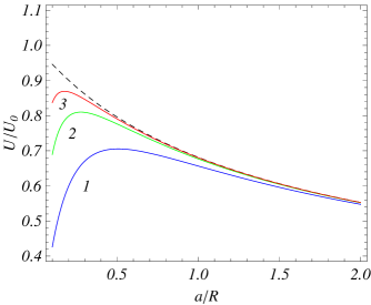
Figure 1: The normalized exact Casimir-Polder potential for a particle outside a cylindrical shell as a function of $a/R$ for $R/\lambda_{A}=1,\>2.5$ and 5 (solid lines 1, 2, and 3, respectively). The dashed line represents the Casimir-Polder potential in the static limit.

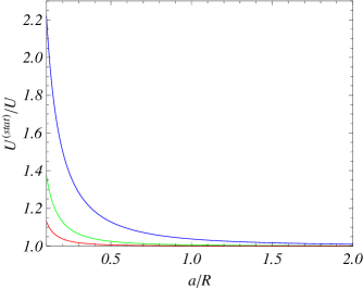
Figure 2: The ratio of exact Casimir-Polder potentials calculated using static and dynamic polarizabilities of a particle as a function of $a/R$ for the same values of $R/\lambda_{A}$, as in Fig. 1, increasing from top to bottom lines.

In Fig. 1 we plot the exact Casimir-Polder energy (28) for a particle outside a shell normalized for $U_{0}$ as a function of $a/R$ using the single-oscillator model [(27) with $\omega_{1}=\omega_{A}$]. Different lines are plotted for $R/\lambda_{A}=1,\>2.5$, and $5$ (lines 1, 2, and 3 respectively), where $\lambda_{A}=2\pi c/\omega_{A}$. The dashed line corresponds to the static limit (29). For instance, for an atom of metastable He^∗ one has 8 $\omega_{A}=1.18$ eV and the cylinder radius corresponding to $R/\lambda_{A}=1$ is equal to $0.95\,\mu$m. As can be seen in Fig. 1, with increasing $R/\lambda_{A}$ the Casimir-Polder energy approaches to the static limit. Note that although lines 1, 2, and 3 around $a/R=0$ demonstrate the same distance dependence (the inverse third power of separation) as does the nonrelativistic limit (i.e., the van der Waals force), they are quite different in nature. Particularly, the van der Waals force does not depend on $c$ whereas the potential (28) in the limit $a/R\to 0$ does. In fact, the nonrelativistic limit cannot be achieved for an ideal metal cylinder. Figure 2 shows the ratio $U^{\rm{(stat)}}/U$ as a function of $a/R$ (the upper, middle and lower lines correspond to $R/\lambda_{A}=1,\>2.5$, and $5$, respectively).

Now we turn to the comparison between the exact Casimir-Polder energy with that obtained using PFA. The latter is given by the expression

$$U_{\rm{PFA}}(a)=-\frac{\hbar c}{16\pi a^{4}}\sqrt{\frac{R}{R+a}}\int_{0}^{\infty}d\zeta\,\alpha(i\omega_{c}\zeta)e^{-\zeta}$$

$$~{}~{}~{}~{}~{}~{}\times\left[2+2\zeta+\zeta^{2}-\frac{a(1+\zeta)}{2(R+a)}\right]$$ (31)

obtained from corresponding equation in 14 by putting the reflection coefficients equal to $\pm 1$, as it holds for ideal metal. In the static limit, (31) leads to

$$U_{\rm{PFA}}(a)=U_{0}(a)\sqrt{\frac{R}{R+a}}\left(1-\frac{1}{6}\frac{a}{R+a}\right),$$ (32)

and for $a/R\ll 1$ one has

$$U_{\rm{PFA}}(a)\approx U_{0}(a)\left(1-\frac{2a}{3R}\right),$$ (33)

to be compared with the exact result (30) obtained in this limiting case. In Fig. 3 we plot the ratio $U/U_{0}$ evaluated in the single-oscillator model by using exact expression (28) (solid lines) and by the PFA, expression (31) (dashed lines). The lines 1 and 2 correspond to $R/\lambda_{A}=1$ and $5$, respectively. As can be seen in Fig. 3, the PFA results are in very good agreement with the exact results. For example, at $a/R=0.1$ the relative deviation between the two results is equal to 1.3% and 0.9% for lines 1 and 2, respectively. The same lines within the region $0.01\leqslant a/R\leqslant 0.1$ are shown on an inset to Fig. 3. At $a/R=0.02$ the relative deviation between the exact and the PFA results does not exceed 0.4%.

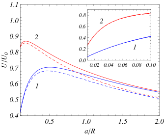
Figure 3: Comparison between the exact and PFA Casimir-Polder potentials for particle-cylinder interaction (the solid and dashed lines, respectively) for $R/\lambda_{A}=1$ and 5 (lines labeled 1 and 2) in the separation region $0.1\leq a/R\leq 2$. The inset shows the region from $a/R=0.01$ to $a/R=0.1$.

6 Microparticle in an interior of cylindrical shell

Here, we present a few computational results for a microparticle inside an ideal metal cylindrical shell. Substituting (27) into (25) and integrating over $\xi$, we find the expression

$$U(r)=\frac{\hbar c}{\pi}\sum_{j}\frac{g_{j}}{\omega_{j}^{2}}\sum_{m=0}^{\infty}{\vphantom{\sum}}^{\!\prime}\,\int_{0}^{\infty}\!\!d\beta\,\beta^{3}\left\{\frac{K_{m}^{\prime}(\beta R)}{I_{m}^{\prime}(\beta R)}\right.$$ (34)

$$\times\frac{F_{m}(\beta r)}{s_{j}(\beta)[s_{j}(\beta)+1]}\left.-\frac{K_{m}(\beta R)}{I_{m}(\beta R)}\left[\,\frac{I_{m}^{2}(\beta r)}{s_{j}(\beta)}+\frac{F_{m}(\beta r)}{s_{j}(\beta)+1}\right]\right\}.$$

In the static limit, similar to (29), one obtains

$$U^{\rm(stat)}(r)=\hbar c\frac{\alpha_{0}}{2\pi}\sum_{m=0}^{\infty}{\vphantom{\sum}}^{\!\prime}\,\int_{0}^{\infty}\!\!d\beta\,\beta^{3}\left\{\frac{K_{m}^{\prime}(\beta R)}{I_{m}^{\prime}(\beta R)}F_{m}(\beta r)\right.$$

$$\left.-\frac{K_{m}(\beta R)}{I_{m}(\beta R)}\left[F_{m}(\beta r)+2I_{m}^{2}(\beta r)\right]\right\}.$$ (35)

The computational results are presented in Fig. 4, where the exact Casimir-Polder energy (34) normalized for $U_{0}$ is plotted as a function of $a/R$ (note that in the interior of a cylindrical shell $a=R-r$ holds). In so doing the single-oscillator model was again used. Similar to Fig. 1, the solid lines from the bottom to the top one correspond to $R/\lambda_{A}=1,\>2.5$, and 5, respectively. The dashed line represents the Casimir-Polder potential in the static limit (35). As is seen in Fig. 4, with increasing $R/\lambda_{A}$ the Casimir-Polder energy for a particle inside a cylindrical shell approaches the static limit. This is in analogy to a particle outside an ideal metal cylindrical shell.

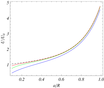
Figure 4: The normalized exact Casimir-Polder potential for a particle inside a cylindrical shell as a function of $a/R$ for $R/\lambda_{A}=1,\>2.5$ and 5 increasing from bottom to top solid lines. The dashed line represents the Casimir-Polder potential in the static limit.

7 Conclusions and Discussion

In the foregoing we have derived the exact Casimir-Polder potential for a polarizable particle placed in an exterior or in an interior of an ideal metal cylindrical shell. Derivation was performed by the Green tensor method. The obtained results for a particle outside the cylindrical shell were compared with obtained by another method and found to be in agreement. Computations were made for particles described by the single-oscillator model. It was shown that at particle-cylinder separations below 0.1$R$ errors introduced by the use of the PFA do not exceed 1.3%. This justifies the application of the PFA for the comparison of the experimental data with theory. We have also investigated the role of dynamic polarizability of the particle. According to our computational results, the static limit is approached for large $a/R$ or $R/\lambda_{A}$. Replacing ideal metal boundary conditions used in expressions (6) and (7) by, for instance, standard electrodynamic continuity conditions or boundary conditions of the Dirac model 18 ; 25a , it is possible to find the respective exact solutions for a particle interacting with a dielectric cylindrical shell or with a single-walled carbon nanotube.

The obtained results can be used in the theory of topological defects, e.g., when there is a cosmic string along the axis of the cylinder. For a cosmic string with the angle deficit $2\pi-\phi_{0}$ ($0\leqslant\phi\leqslant\phi_{0}$), the formulae for the Casimir-Polder potential are obtained from (19) and (25) by the replacement $m\rightarrow qm$ and adding the factor $q$, where $q=2\pi/\phi_{0}$ (for the corresponding eigenfunctions see 19 ). Note that the conducting cylindrical surface can be considered as a simple model of superconducting string core. Superconducting strings are predicted in a wide class of field theories and they are sources of a number of interesting astrophysical effects such as generation of synchrotron radiation, cosmic rays, and relativistic jets.

References

- (1) H.B.G. Casimir, D. Polder, Phys. Rev. 73, 360 (1948)
- (2) H.B.G. Casimir, Proc. K. Ned. Akad. Wet. 51, 793 (1948)
- (3) P.S. Wesson, Five-Dimensional Physics: Classical and Quantum Consequencies of Kaluza-Klein Cosmology (World Scientific, Singapore, 2006)
- (4) E. Elizalde, S.D. Odintsov, A. Romeo, A.A. Bytsenko, S. Zerbini, Zeta Regularization Techniques with Applications (World Scientific, Singapore, 1994)
- (5) A. Vilenkin, E.P.S. Shellard, Cosmic Strings and Other Topological Defects (Cambridge University Press, Cambridge, 1994)
- (6) G.L. Klimchitskaya, U. Mohideen, V.M. Mostepanenko, Rev. Mod. Phys. 81, 1827 (2009)
- (7) H. Friedrich, J. Trost, Phys. Rep. 397, 359 (2004)
- (8) S. Bellucci, A.A. Saharian, Phys. Rev. D 79, 085019 (2009)
- (9) S. Bellucci, A.A. Saharian, Phys. Rev. D 80, 105003 (2009)
- (10) T. Emig, R.L. Jaffe, M. Kardar, A. Scardicchio, Phys. Rev. Lett. 96, 080403 (2006).
- (11) M. Bordag, Phys. Rev. D 73, 125018 (2006).
- (12) B.V. Derjaguin, Kolloid. Z. 69, 155 (1934).
- (13) J. Błocki, J. Randrup, W.J. Swiatecki, C.F. Tsang, Ann. Phys. (NY) 105, 427 (1977)
- (14) R.S. Decca, E. Fischbach, G.L. Klimchitskaya, D.E. Krause, D. López, V.M. Mostepanenko, Phys. Rev. D 79, 124021 (2009)
- (15) E. Fischbach, G.L. Klimchitskaya, D.E. Krause, V.M. Mostepanenko, Eur. Phys. J. C 68, 223 (2010)
- (16) B. Geyer, G.L. Klimchitskaya, V.M. Mostepanenko, Phys. Rev. A 82 032513 (2010)
- (17) C. Eberlein, R. Zietal, Phys. Rev. A 80, 012504 (2009)
- (18) S. A. Ellingsen, S. Y. Buhmann, S. Scheel, Phys. Rev. A 82, 032516 (2010)
- (19) S.Y. Buhmann, D.-G. Welsch, Progr. Quant. Electronics 31, 51 (2007)
- (20) A.A. Saharian, The Generalized Abel-Plana Formula with Applications to Bessel Functions and Casimir Effect (Yerevan State University Publishing House,Yerevan, 2008); Preprint ICTP/2007/082; arXiv:0708.1187
- (21) H. Nha, W. Jhe, Phys. Rev. A 56, 2213 (1997)
- (22) M. Bordag, G.L. Klimchitskaya, U. Mohideen, V.M. Mostepanenko, Advances in the Casimir Effect (Oxford University Press, Oxford, 2009)
- (23) J.F. Babb, G.L. Klimchitskaya, V.M. Mostepanenko, Phys. Rev. A 70, 042901 (2004)
- (24) A.O. Caride, G.L. Klimchitskaya, V.M. Mostepanenko, S.I. Zanette, Phys. Rev. A 71, 042901 (2005)
- (25) E.V. Blagov, G.L. Klimchitskaya, V.M. Mostepanenko, Phys. Rev. B 75, 235413 (2007)
- (26) M. Bordag, I.V. Fialkovsky, D.M. Gitman, D.V. Vassilevich, Phys. Rev. B 80, 245406 (2009)
- (27) Yu.V. Churkin, A.B. Fedortsov, G.L. Klimchitskaya, V.A. Yurova, Phys. Rev. B 82, 165433 (2010)
- (28) E.R. Bezerra de Mello, V.B. Bezerra, A.A. Saharian, Phys. Lett. B 645, 245 (2007)