Feedback Reduction for Random Beamforming in Multiuser MIMO Broadcast Channel

Abstract

For the multiuser multiple-input multiple-output (MIMO) downlink channel, the users feedback their channel state information (CSI) to help the base station (BS) schedule users and improve the system sum rate. However, this incurs a large aggregate feedback bandwidth which grows linearly with the number of users. In this paper, we propose a novel scheme to reduce the feedback load in a downlink orthogonal space division multiple access (SDMA) system with zero-forcing receivers by allowing the users to dynamically determine the number of feedback bits to use according to multiple decision thresholds. Through theoretical analysis, we show that, while keeping the aggregate feedback load of the entire system constant regardless of the number of users, the proposed scheme almost achieves the optimal asymptotic sum rate scaling with respect to the number of users (also known as the multiuser diversity). Specifically, given the number of thresholds, the proposed scheme can achieve a constant portion of the optimal sum rate achievable only by the system where all the users always feedback, and the remaining portion (referred to as the sum rate loss) decreases exponentially to zero as the number of thresholds increases. By deriving a tight upper bound for the sum rate loss, the minimum number of thresholds for a given tolerable sum rate loss is determined. In addition, a fast bit allocation method is discussed for the proposed scheme, and the simulation results show that the sum rate performances with the complex optimal bit allocation method and with the fast algorithm are almost the same. We compare our multi-threshold scheme to some previously proposed feedback schemes. Through simulation, we demonstrate that the proposed scheme can reduce the feedback load and utilize the limited feedback bandwidth more effectively than the existing feedback methods.

I Introduction

Multiple-input multiple-output (MIMO) technologies can provide spatial diversity in wireless fading channels to improve the communication quality. In particular, recent studies have shown that the sum rates of MIMO systems can be increased when the base station (BS) communicates with multiple users simultaneously [1]. For the downlink broadcast channel employing multiple antennas, it has been shown recently that dirty paper coding (DPC) [2] achieves the capacity [3]. However, this capacity achieving scheme is difficult to derive and has a high encoding/decoding complexity. Thus, several works resorted to the more practical (but suboptimal) space division multiple access (SDMA) based designs. For example, zero-forcing beamforming (ZF-BF) was shown in [4] to achieve the optimal sum rate growth. However, both the DPC and the ZF schemes require perfect channel state information (CSI) feedback from the users to the BS to achieve the optimal performance. This may result in high feedback load and is not practical.

In [5, 6], a model was proposed to analyze the sum rate loss due to imperfect (quantized) CSI. In the system considered there, each user quantizes the channel vector to one of the $N=2^{B}$ quantization vectors and feeds back the codebook index using $B$ bits to the BS to capture the spatial direction and magnitude of the channel. To reduce the feedback load, the orthogonal random beamforming (ORB) scheme [7] can be used. In the ORB scheme, the BS transmits through orthogonal beamforming vectors to the users, and each user only needs to feedback its received signal-to-interference-plus-noise ratios (SINR) on different orthogonal beamforming vectors for the purpose of scheduling. It was shown in [7] that the ORB exhibits the same sum rate growth as the DPC and the ZF-BF based schemes when the number of users is large.

There are other previous works that sought to reduce the feedback load at the scheduling stage. In [8], a threshold was set according to the scheduling outage probability such that a user did not need to feedback when its CSI is below the threshold. This method reduces the system feedback load without affecting the scheduling performance much. In [9], multiple thresholds were set, and the scheduler utilized a polling process to select the best feedback threshold from these thresholds to further reduce the aggregate feedback load. However, the drawback of this scheme is the large delay incurred by the polling process. In [10], another scheme was proposed to reduce the feedback load of the ZF-BF systems through two-stage feedback. In the first stage, each user feeds back the coarsely quantized version of its CSI, and thus the BS has some information to determine which users to schedule. The BS then broadcasts to the scheduled users and asks them to feedback finer CSI to achieve good ZF-BF performance in the second stage. The drawback of this scheme is also the delay incurred by the two-stage feedback process.

From the above discussion, it is clear that the feedback load of multiuser MIMO systems can be reduced if the scheduling mechanism is taken into consideration. However, most existing works only use the scheduling mechanism to control the amount of feedback, but not incorporate the properties of scheduling into the CSI quantization design. In view of this, in this paper we propose to reduce the feedback load by incorporating the scheduling mechanism in both the determination of the amount to feedback and the CSI quantization. The proposed scheme divides the range of CSI into multiple regions according to the order statistics of the received signal-to-noise ratio (SNR) which reflect the properties of scheduling. Each region corresponds to a range of SNR, and is quantized with a specific number of bits to further assist scheduling and link adaptation. The CSI feedback thus consists of two parts: one indicating the region that the received SNR falls in, and the other being the quantized result of that region. For a given number of regions, we derive a tight upper bound for the sum rate loss of the proposed scheme as compared to systems with perfect CSI feedback from all users. Then, for any given tolerable sum rate loss of the system, the minimum number of regions required is derived. For example, the proposed scheme with four regions is good enough to keep the sum rate loss smaller than $0.25$ bps/Hz for the number of users less than 100. In addition, the aggregate feedback load and the multiuser diversity using the proposed scheme are also investigated. Our theoretical analysis shows that, in contrast to the existing feedback schemes whose aggregate feedback loads increase with the number of users, with a given number of regions, the proposed scheme has a constant feedback load regardless of the number of users. Moreover, while keeping the feedback load constant, the proposed scheme almost achieves the optimal asymptotic sum rate scaling with respect to the number of users (that is, the multiuser diversity). Specifically, given the number of regions, the proposed scheme can achieve a constant portion of the optimal sum rate achievable only by the system where all the users always feedback, and the sum rate loss decreases exponentially to zero as the number of regions increases. Through simulation, we verify these analytical results, and demonstrate that the proposed scheme can reduce the feedback load and utilize the limited feedback bandwidth more effectively than the existing feedback methods. A fast bit allocation method that assigns different numbers of quantization bits to different regions is also discussed. The simulation results show that the sum rate performances with the complex optimal bit allocation method and with the fast algorithm are almost the same.

Note that the required information for the proposed scheme to operate, such as the SNR statistics and the number of users, are usually known at the BS. Thus, in practices, the BS can compute the region thresholds and broadcast to the users periodically, or broadcast the parameters of the SNR statistics and the number of users periodically to the users to let them derive the thresholds.

The remainder of this paper is organized as follows. Section II describes the system model and briefs the order statistics. Section III introduces the proposed feedback scheme and analyzes its sum rate loss and multiuser diversity. In Section IV, the bit allocation problem is discussed along with the feedback load analysis. We then give the simulation results in Section V and conclude the paper in Section VI.

Notation: Vectors and matrices are denoted by boldface lower case and capital letters, respectively. $\mathbb{E}\{\cdot\}$ refers to expected values of a random variable. ${\mathbf{X}}^{T}$ $({\mathbf{x}}^{T})$ stands for the transpose of matrix $\mathbf{X}$ (vector ${\mathbf{x}}$), and ${\mathbf{X}}^{*}$ $({\mathbf{x}}^{*})$ stands for the conjugate transpose of matrix $\mathbf{X}$ (vector ${\mathbf{x}}$). Moreover, ${\mathbf{X}}^{{\dagger}}$ denotes the pseudo-inverse ${\mathbf{X}}^{*}({\mathbf{X}}{\mathbf{X}}^{*})^{-1}$. The function $\lceil x\rceil$ represents the smallest integer $\geq x$. $\log$ and $\ln$ are the logarithms with base $2$ and $e$, respectively.

II System Model

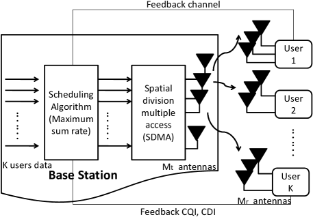
The multiuser MIMO downlink system model is shown in Fig.1 where the BS is equipped with $M_{t}$ antennas. There are $K$ users in the system and each user has $M_{r}$ receive antennas. We consider a full buffer traffic model, that is, each user always has data in the buffer to transmit. According to the ORB strategy for multiuser transmission, the BS uses a precoding matrix ${{\mathbf{W}}=[{\mathbf{w}}_{1},{\mathbf{w}}_{2},\ldots,{\mathbf{w}}_{M_{t}}]}$, where ${\mathbf{w}}_{i}\in{{\mathbb{C}}^{M_{t}}},i=1,2,\ldots,M_{t}$, are random orthogonal vectors generated from isotropic distribution [11]. The received signal at the $k$-th user can be mathematically described as:

$${\mathbf{y}}_{k}={\mathbf{H}}_{k}{\mathbf{W}}{\mathbf{s}}+{\mathbf{n}}_{k},$$ (1)

where ${\mathbf{H}}_{k}$ is the $M_{r}\times M_{t}$ complex Gaussian channel matrix between the BS and the $k$-th user, ${\mathbf{n}}_{k}$ is the $M_{r}\times 1$ additive white Gaussian noise (AWGN) vector at the $k$-th user. The entries of ${\mathbf{H}}_{k}$ and ${\mathbf{n}}_{k}$ are assumed to be independent identically distributed (i.i.d.) complex Gaussian with zero mean and unit variance. In addition, the channel matrices for different users are assumed to be independent. Note that in this paper we consider only identical channel distributions for the users for the simplicity of demonstrating the idea. The more practical situations where the users have different channel statistics or distributions are more intricate, and are discussed in [12]. The vector ${\mathbf{s}}=[{{s}}_{1},{{s}}_{2},\ldots,{{s}}_{M_{t}}]^{T}$ is the $M_{t}\times 1$ vector of the transmitted signal. It is assumed that the feedback channel is error-free and delay-free. The total transmitted power is a constant $P_{t}$ so that ${{\mathbb{E}}\{\mathbf{s}^{*}\mathbf{s}\}}=P_{t}$. Under the equal power assumption of the ORB, each beam is equally allocated with power $\rho=P_{t}/M_{t}$.

Figure 1: Multiuser MIMO downlink system model.

We consider zero-forcing receivers. The received signal after the zero-forcing filter is given by

$${({\mathbf{H}}_{k}{\mathbf{W}})}^{\dagger}{\mathbf{y}}_{k}={\mathbf{s}}+{({\mathbf{H}}_{k}{\mathbf{W}})}^{\dagger}{\mathbf{n}}_{k}.$$ (2)

Therefore, the received SNR of the $m$-th signal $s_{m}$ at the $k$-th user with the ZF receiver is given by

$$SNR_{m,k}=\frac{\rho}{[(({\mathbf{H}}_{k}{\mathbf{W}})^{*}({\mathbf{H}}_{k}{\mathbf{W}}))^{-1}]_{m}}$$ (3)

where $[{\mathbf{A}}]_{m}$ denotes the $m$-th diagonal element of matrix $\mathbf{A}$. Assuming that $M_{r}\geq M_{t}$, it is well known that $SNR_{m,k}$ is a chi-square random variable with $2(M_{r}-M_{t}+1)$ degrees of freedom [13]. For simplicity, we let $X_{m,k}=SNR_{m,k}$ and then the probability density function (PDF) of $X_{m,k}$ can be expressed as

$$f_{X_{m,k}}{(x)}=\frac{e^{-\frac{x}{\rho}}}{\rho(M_{r}-M_{t})!}\begin{array}[]{cc}({\frac{x}{\rho})}^{M_{r}-M_{t}},&x>0.\\ \end{array}$$ (5)

Consequently, the cumulative distribution function (CDF) of $X_{m,k}$ is given by

$$F_{X_{m,k}}{(x)}=1-\frac{\Gamma(M_{r}-M_{t}+1,\frac{x}{\rho})}{(M_{r}-M_{t})!},\forall m,k,$$ (6)

where $\Gamma(a,x)=\int_{x}^{\infty}t^{a-1}e^{-t}dt$ is the upper incomplete gamma function. According to (5), when the transmitter and the receiver have the same number of antennas, $X_{m,k}$ has an exponential distribution with parameter $1/\rho$. For simplicity of the derivation, we will consider this $M_{r}=M_{t}$ case for the ORB system. Extension to the other cases is straightforward, but the mathematical expressions are more complicated.

We consider that the maximum sum rate scheduling algorithm is employed at the BS. That is, on each beam direction, the BS selects, among the users who have fed back their CSIs, the user that has the best channel to transmit to. If none of the users has fed back the CSI, the BS randomly selects one user to transmit to. Due to the symmetric property, we drop the direction index $m$ of $X_{m,k}$, and let $X_{k}$ represent the SNR of user $k$ for a ceratin beam. Let ${X_{(1)}^{K},X_{(2)}^{K},\ldots,X_{(K)}^{K}}$, be the order statistics of i.i.d. continuous random variables $X_{1},X_{2},\ldots,X_{K}$, with the common PDF (5) in decreasing order, i.e., ${X_{(1)}^{K}\geq X_{(2)}^{K}\geq\cdots\geq X_{(K)}^{K}}$. The PDF and CDF of $X_{(j)}^{K}$, respectively, are given by[14]:

$$F_{X_{(j)}^{K}}{(x)}=\sum_{i=K-(j-1)}^{K}{\frac{K!\{F_{X_{m,j}}(x)\}^{i}\{1-F_{X_{m,j}}(x)\}^{K-i}}{(i)!(K-i)!}},-\infty<x<\infty,$$ (7)

$$f_{X_{(j)}^{K}}{(x)}=\frac{K!f_{X_{m,j}}(x)\{F_{X_{m,j}}(x)\}^{K-j}\{1-F_{X_{m,j}}(x)\}^{j-1}}{(j-1)!(K-j)!},-\infty<x<\infty.$$ (8)

With the order statistics, the sum rate using the maximum sum rate scheduling algorithm can be computed. As a simple example, if every user has the probability $P_{f}$ to feedback the CSI for a particular beam direction to the BS, and the feedback events are independent of the value of the CSI and independent from user to user and from beam to beam, the sum rate can be obtained by

$$R(K,P_{f})=M_{t}{\mathbb{E}}\left\{\sum_{n=1}^{K}\frac{K!{P_{f}}^{n}{(1-P_{f})}^{K-n}}{n!(K-n)!}\log(1+X_{(1)}^{n})+(1-P_{f})^{K}\log(1+X_{k})\right\}$$ (9)

where the second term is the rate when no user feeds back to the BS and the BS randomly schedules one user $k$ on a ceratin beam.

III The Multi-threshold Feedback Scheme

For the scheme in [8], if the SNR of a user is greater than the outage threshold, the user feeds back $B_{Q}$ bits to represent the received SNR. Otherwise it does not feedback. The threshold is derived according to a pre-determined scheduling outage probability (where “scheduling outage” refers to the situation when none of the users feeds back), but not directly related to the scheduling mechanism. Since the maximum sum rate scheduler selects users according to their SNR orders, it is more meaningful to set the threshold according to the order statistics of the received SNR.

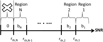
The basic idea of our proposed scheme is to let a user compare its received SNR with the thresholds derived from the order statistics. The user can thus guess its most possible rank among all the users, and, if its rank is high enough to make its chance to be scheduled high, it feeds back its SNR. Otherwise the user does not feedback in order to save the reverse link resource and avoid interfering the other users’ reverse link transmission. Note that there might be errors in the statistical inference by the individual users about their SNR ranks. These errors may result in the situation where the users who actually have high SNRs do not feedback, and the BS does not have proper users to select from. To make up for the sum rate loss due to this situation, we allow the users with several (guessed) ranks to feedback. Therefore, for each beam direction, a set of $N$ thresholds $R_{th}=\{r_{th,1},r_{th,2},\ldots,r_{th,N}\}$ is set (see Fig. 2) according to the order statistics of the received SNR. Let $r_{th,0}=\infty$. For SNR region $i$ bounded by the adjacent thresholds as $[r_{th,i},r_{th,i-1})$, $b_{i}$ additional quantization bits are used to help the BS differentiate users whose SNRs fall in that region, and make better link adaptation. According to the importance of the SNR regions to the sum rate, $b_{i},i=1,\ldots,N$, (to be optimized later) are usually in non-increasing order. When the received SNR is higher than $r_{th,N}$, the user feeds back its rank and the additional quantization bits. Otherwise the user does not feedback at all.

III-A Derivation of Multiple Thresholds

III-A1 i.i.d. case

When user $k$ has on its $m$-th beam $SNR_{m,k}=snr_{m,k}$ and the users have i.i.d. SNR distribution, the probability that user $k$’s SNR on the $m$-th beam direction is ranked the $p$-th among all the users is

$$P\{X_{k}=X_{(p)}^{K}|X_{k}=snr_{m,k}\}$$ (10)

$$= \frac{(K-1)!\{F_{X_{m,k}}(snr_{m,k})\}^{K-p}\{1-F_{X_{m,k}}(snr_{m,k})\}^{p-1}}{(K-p)!(p-1)!},$$

and satisfies

$$\sum_{p=1}^{K}P\{X_{k}=X_{(p)}^{K}|X_{k}=snr_{m,k}\}=1.$$ (11)

where $F_{X_{m,k}}(x)$ is defined in (6).

Figure 2: Multi-threshold feedback model.

For example, the probability that user $k$ has on its $m$-th beam $SNR_{m,k}=snr_{m,k}$ which is the highest SNR among all the users on the $m$-th beam is

$${\frac{P\{X_{(1)}^{K}=snr_{m,k}\}}{P\{X_{k}=snr_{m,k}\}}}=\left(F_{X_{m,k}}(snr_{m,k})\right)^{K-1}.$$ (12)

With $SNR_{m,k}=snr_{m,k}$, user $k$ can infer its most possible rank among the users on the $m$-th beam as

$$rank(snr_{m,k})=\arg\max_{p=1,\ldots,K}P\{X_{k}=X_{(p)}^{K}|X_{k}=snr_{m,k}\}.$$ (13)

III-A2 non-i.i.d. case

In practical systems, the users may be at different distances to the BS. Thus the CDFs of the users’ SNRs $F_{X_{m,j}}(x),j=1,2,\ldots,K$, may not be identical as in (6). Assuming that the users’ SNRs are independent, the probability that user $k$’s SNR on the $m$-th beam direction is ranked the $p$-th among all the users becomes

$$P\{X_{k}=X_{(p)}^{K}|X_{k}=snr_{m,k}\}$$ (14)

$$= \sum_{s(\cdot)\in{\cal S}}\left\{\prod_{j=1}^{K-p}F_{X_{m,s(j)}}(snr_{m,k})\prod_{j=K-p+1}^{K-1}\left(1-F_{X_{m,s(j)}}(snr_{m,k})\right)\right\},$$

where ${\cal S}$ is a set of permutation functions defined by

$${\cal S} = \left\{s:\{1,\ldots,K-1\}\rightarrow\{1,\ldots,k-1,k+1,\ldots,K\}~{}|~{}s(\cdot)\mbox{ invertible},\right.$$

$$\left.s(1)<\cdots<s(K-p)\mbox{ and }s(K-p+1)<\cdots<s(K-1)\right\},$$

where the last two conditions are to avoid multiple counting of the same combination. The most possible rank of user $k$ can again be found using (13).

To this end, the regions in Fig. 2 are defined such that for all the SNR values in region $j$, i.e., $\forall~{}snr_{m,k}\in[r_{th,j},r_{th,j-1})$, $rank(snr_{m,k})=j$. Thus the number of regions $N$ must be no larger than the number of users $K$. The corresponding thresholds $r_{th,j},j=1,2,\ldots,N$, can then be determined accordingly. All the thresholds can be computed off-line as long as the number of users and the channel statistics are known. The values of the thresholds can be updated periodically according to the system configuration and channel statistics possibly broadcasted by the BS.

In this paper we will consider only i.i.d. SNR distributions for the simplicity of demonstrating the idea. The non-i.i.d. case is much more intricate, and is handled separately in [12]. If a user finds its SNR on a beam lower than $r_{th,N}$, then no feedback is sent for that beam. Otherwise, the user feeds back $B_{R}=\lceil{\log_{2}(N)}\rceil$ bits to indicate its most possible rank on that beam. In order to account for the situation where there are more than one users reporting to have the same rank, each region $j$ is further quantized with $b_{j}$ bits which are also fed back together with the “rank” bits.

Due to the symmetric assumption that the users suffer i.i.d. Rayleigh fading processes, also due to the ORB, the same set of thresholds applies to all users and all beam directions. Since $rank(snr_{m,k})=j$ when $snr_{m,k}\in[r_{th,j},r_{th,j-1})$, $rank(snr_{m,k})=j+1$ when $snr_{m,k}\in[r_{th,j+1},r_{th,j})$, and the probability $P\{X_{k}=X_{(p)}^{K}|X_{k}=snr_{m,k}\}$ in (10) is a continuous function of $snr_{m,k}$ for $p=1,2,\ldots,K$, using (10) and (13) we have

$$P\{X_{k}=X_{(j)}^{K}|X_{k}=r_{th,j}\}=P\{X_{k}=X_{(j+1)}^{K}|X_{k}=r_{th,j}\}$$

$$\Leftrightarrow \frac{F_{X_{m,k}}(r_{th,j})}{K-j}=\frac{1-F_{X_{m,k}}(r_{th,j})}{j}$$

$$\Leftrightarrow j\left(1-e^{-\frac{r_{th,j}}{\rho}}\right)=(k-j)e^{-\frac{r_{th,j}}{\rho}}$$

$$\Leftrightarrow r_{th,j}={\rho}\ln\left(\frac{K}{j}\right),~{}~{}~{}j=1,2,\ldots,N.$$ (15)

Then

$$P\{X_{k}\in[r_{th,j},r_{th,j-1})\}=\frac{1}{K},~{}~{}j=1,2,\ldots,N.$$ (16)

In other words, the probability for a user to infer itself as being ranked the $j$th place on a certain beam direction is ${\frac{1}{K}}$, for all $j=1,2,\ldots,N$, with $N\leq K$. This is very intuitive because each user has the same probability ${\frac{1}{K}}$ of being ranked the $j$th place, $j=1,2,\ldots,K$, due to the symmetric assumption of the users’ SNR distributions. Therefore, the probability $P_{f}$ for a user to feedback is

$$\ P_{f}=1-F_{X_{m,k}}(r_{th,N})=e^{-\frac{r_{th,N}}{\rho}}=\frac{N}{K}.$$ (17)

III-B Minimum Number of Regions and Sum Rate Loss Analysis

One important issue regarding the multi-threshold design is the number of regions to be applied. The number of regions affects the sum rate loss. If the number of regions increases, which results in higher feedback load, the sum rate loss will decrease. Thus, for a given tolerable sum rate loss, we should apply the minimum number of regions required to minimize the feedback load.

Let the rate loss event be defined as when all users’ SNRs on a certain beam is smaller than the threshold $r_{th,N}$, and the BS randomly schedules one user because none has fed back. Note that this event is called the scheduling outage event in [8]. The probability of the rate loss event is then

$$\ P_{L}=P\{X_{(1)}^{K}<r_{th,N}\}=\left(1-e^{-\frac{r_{th,N}}{\rho}}\right)^{K}.$$ (18)

Without loss of generality, assume that user $k$ is selected by the BS in a rate loss event. The sum rate loss compared to the case when the users always feed back is

$$\triangle R(K,N) = M_{t}\mathbb{E}\left\{\log(1+X_{(1)}^{K})-\log(1+X_{k})~{}|~{}X_{(1)}^{K}<r_{th,N}\right\}P_{L}$$ (19)

$$\leq M_{t}\mathbb{E}\left\{\log\left(1+\left(X_{(1)}^{K}-X_{k}\right)\right)~{}|~{}X_{(1)}^{K}<r_{th,N}\right\}P_{L}$$

$$\leq M_{t}\log\left(1+{\mathbb{E}}\left\{\left(X_{(1)}^{K}-X_{k}\right)~{}|~{}X_{(1)}^{K}<r_{th,N}\right\}\right)P_{L}$$

$$\triangleq \triangle R_{U}(K,N),$$

where the inequalities are due to the convexity of the rate function and Jensen’s inequality. By using (15),

$${\mathbb{E}}\left\{\left(X_{(1)}^{K}-X_{k}\right)|X_{(1)}^{K}<r_{th,N}\right\}$$

$$=\int_{0}^{r_{th,N}}\frac{xK\frac{1}{\rho}e^{-\frac{x}{\rho}}\left(1-e^{-\frac{x}{\rho}}\right)^{K-1}}{\left(1-e^{-\frac{r_{th,N}}{\rho}}\right)^{K}}dx-\int_{0}^{r_{th,N}}\frac{x\frac{1}{\rho}e^{-\frac{x}{\rho}}\left(1-e^{-\frac{r_{th,N}}{\rho}}\right)^{K-1}}{\left(1-e^{-\frac{r_{th,N}}{\rho}}\right)^{K}}dx$$

$$=\frac{\displaystyle\frac{K}{\rho}\displaystyle\sum_{t=0}^{K-1}\frac{(-1)^{t}(K-1)!}{t!(K-t-1)!}\left(\begin{array}[]{c}\displaystyle\frac{1-{(\frac{N}{K})}^{{c}{\rho}}}{c^{2}}-\frac{{\rho}\left(\ln\frac{K}{N}\right){(\frac{N}{K})}^{{c}{\rho}}}{c}\\ \end{array}\right)}{(1-\frac{N}{K})^{K}}-{\rho}\left(1-\frac{\left(\ln\frac{K}{N}\right)\left(\frac{N}{K}\right)}{(1-\frac{N}{K})}\right)$$ (21)

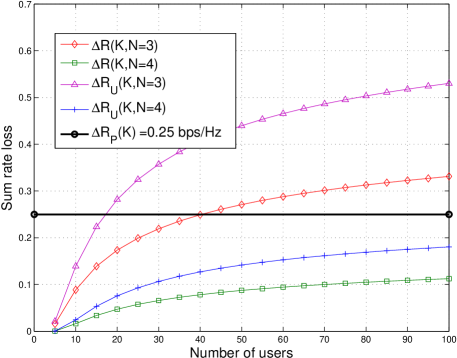
where $\displaystyle c=\frac{(1+t)}{\rho}$. Using (19) and (21), the minimum number of regions required for a given tolerable sum rate loss $\bigtriangleup R_{P}(K)$ can be effectively approximated by comparing the sum rate loss upper bound $\triangle R_{U}(K,N)$ with $\bigtriangleup R_{P}(K)$. Fig. 3 compares the sum rate loss upper bound with the actual sum rate loss obtained by simulation, and shows that the sum rate loss upper bound (19) with (21) is tight (within 0.1 bps/Hz) when the number of regions is large. This figure also shows that four regions are enough to keep the sum rate loss smaller than the tolerable sum rate loss $\bigtriangleup R_{P}(K)=0.25$ bps/Hz when the number of users is less than 100.

Figure 3: Sum rate loss versus the number of users. $\bigtriangleup R_{P}(K,N)=0.25$ bps/Hz, $\rho=10$ dB

Another important issue is how much the sum rate can be increased when the number of regions is increased by one. By (15) and (18), when the number of regions increases from $N$ to $N+1$, the probability of the rate loss event is reduced by

$$P_{I} =P\{r_{th,N+1}\leq X_{(1)}^{K}<r_{th,N}\}=\left(\begin{array}[]{c}\displaystyle\frac{K-N}{K}\\ \end{array}\right)^{K}-\left(\begin{array}[]{c}\displaystyle\frac{K-N-1}{K}\\ \end{array}\right)^{K}.$$ (24)

Note that when $r_{th,N+1}\leq X_{(1)}^{K}<r_{th,N}$, the system with $N+1$ regions will schedule the user with the highest SNR, while the system with $N$ regions will randomly schedule a user. Otherwise, the two systems have the same scheduling operations. Without loss of generality, assume that the randomly scheduled user is user $k$. When the number of regions increases from $N$ to $N+1$, the sum rate increment $\triangle R_{in}(K,N)$ can be upper bounded by

$$\triangle R_{in}(K,N) = M_{t}\mathbb{E}\left\{\log(1+X_{(1)}^{K})-\log(1+X_{k})~{}|~{}r_{th,N+1}\leq X_{(1)}^{K}<r_{th,N}\right\}P_{I}$$ (25)

$$\leq M_{t}\mathbb{E}\left\{\log\left(1+\left(X_{(1)}^{K}-X_{k}\right)\right)~{}|~{}r_{th,N+1}\leq X_{(1)}^{K}<r_{th,N}\right\}P_{I}$$

$$\leq M_{t}\log\left(1+{\mathbb{E}}\left\{\left(X_{(1)}^{K}-X_{k}\right)~{}|~{}r_{th,N+1}\leq X_{(1)}^{K}<r_{th,N}\right\}\right)P_{I}$$

$$\triangleq \triangle R_{in,U}(K,N),$$

where

$${\mathbb{E}}\left\{\left(X_{(1)}^{K}-X_{k}\right)|r_{th,N+1}\leq X_{(1)}^{K}<r_{th,N}\right\}=\frac{1}{P_{I}}\left\{\int_{r_{th,N+1}}^{r_{th,N}}xK\frac{1}{\rho}e^{-\frac{x}{\rho}}(1-e^{-\frac{x}{\rho}})^{K-1}dx\right.$$

$$-\Bigg{(}\int_{0}^{r_{th,N+1}}P_{A}\frac{x}{\rho}e^{-\frac{x}{\rho}}dx\left.+\int_{r_{th,N+1}}^{r_{th,N}}P_{B}\frac{x}{\rho}e^{-\frac{x}{\rho}}dx\Bigg{)}\right\}$$

$$=\frac{1}{P_{I}}\left\{\frac{K}{\rho c^{2}}\sum_{t=0}^{K-1}\frac{(-1)^{t}(K-1)!}{t!(K-t-1)!}\left[\left(cr_{th,N+1}+1\right)e^{-cr_{th,N+1}}-\left(cr_{th,N}+1\right)e^{-cr_{th,N}}\right]\right.$$

$$\left.-\left(P_{A}\left[\rho-\left(\rho+r_{th,N+1}\right)e^{-\frac{r_{th,N+1}}{\rho}}\right]+P_{B}\left[\left(\rho+r_{th,N+1}\right)e^{-\frac{r_{th,N+1}}{\rho}}-\left(\rho+r_{th,N}\right)e^{-\frac{r_{th,N}}{\rho}}\right]\right)\right\}$$

where

$$P_{A}=\left[(1-e^{-\lambda r_{th,N}})^{K-1}-(1-e^{-\lambda r_{th,N+1}})^{K-1}\right],$$

$$P_{B}=\left(1-e^{-\lambda r_{th,N}}\right)^{K-1}.$$

Furthermore, $\triangle R_{in}(K,N)$ can be lower bounded by

$$\triangle R_{in}(K,N) = M_{t}\mathbb{E}\left\{\log(1+X_{(1)}^{K})-\log(1+X_{k})~{}|~{}r_{th,N+1}\leq X_{(1)}^{K}<r_{th,N}\right\}P_{I}$$ (26)

$$> M_{t}\left[\log\left(1+r_{th,N+1}\right)-\mathbb{E}\left\{\log\left(1+X_{k}\right)~{}|~{}r_{th,N+1}\leq X_{(1)}^{K}<r_{th,N}\right\}\right]P_{I}$$

$$\geq M_{t}\left[\log\left(1+r_{th,N+1}\right)-\log\left(1+{\mathbb{E}}\left\{X_{k}~{}|~{}r_{th,N+1}\leq X_{(1)}^{K}<r_{th,N}\right\}\right)\right]P_{I}$$

$$\triangleq \triangle R_{in,L}(K,N).$$

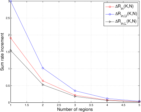
Fig. 4 compares the simulated sum rate increment with the upper bound (25) and lower bound (26) for different numbers of regions $N$ when the number of users is $K=100$. As in Fig. 3, the bounds become tighter when $N$ is large. In addition, the sum rate increment gets smaller as the number of regions gets larger. Eventually the sum rate increment will approach zero (when $N=K$, the users always feedback and the sum rate increment is exactly zero).

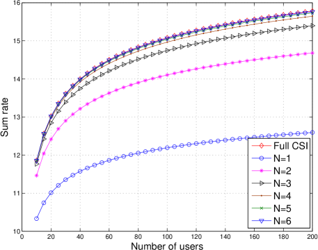
Fig. 5 shows the simulation results of the sum rate for different numbers of regions when the number of users increases. It is shown that the sum rate increases with both the number of users and the number of regions. Both the sum rate loss and the the sum rate increment decrease with the number of regions as already shown in Fig. 3 and Fig. 4, respectively. When the number of regions is larger than four, the sum rate achieved by the multi-threshold scheme is very close to the sum rate with full CSI.

Figure 4: The sum rate increment when the number of regions is increased from $N$ to $N+1$. $\rho=10$ dB, $K$=100

Figure 5: Sum rate performance of the multi-threshold scheme with different numbers of regions. $\rho=10$ dB.

III-C Multiuser Diversity Using the Multi-threshold Scheme

In this section, we characterize the asymptotic sum rate scaling of the multi-threshold feedback scheme with respect to the number of users, that is, the multiuser diversity. The sum rate using this scheme can be expressed as

$$R(K,N) = M_{t}P\{r_{th,N}\leq X_{(1)}^{K}<\infty\}\mathbb{E}\left\{\log(1+X_{(1)}^{K})~{}|~{}r_{th,N}\leq X_{(1)}^{K}<\infty\right\}$$ (27)

$$+ M_{t}P\{0\leq X_{(1)}^{K}<r_{th,N}\}\mathbb{E}\left\{\log(1+X_{k})~{}|~{}0\leq X_{(1)}^{K}<r_{th,N}\right\}.$$

When the number of users is large, this sum rate exhibits the following property.

Theorem 1

Let $M_{t}$, $\rho$, $N$ be given, and the lowest threshold $r_{th,N}={\rho}\ln(K/N)$. The achievable sum rate $R(K,N)$ of the multi-threshold feedback scheme satisfies

$$\lim_{K\rightarrow\infty}\frac{R(K,N)}{M_{t}\log\log K}=1-e^{-N}.$$

Proof:

The sum rate can be lower bounded by

$$R(K,N) \geq M_{t}P\{r_{th,N}\leq X_{(1)}^{K}<\infty\}\mathbb{E}\left\{\log(1+X_{(1)}^{K})~{}|~{}r_{th,N}\leq X_{(1)}^{K}<\infty\right\}$$ (28)

$$\geq M_{t}\left(1-P_{L}\right)\log(1+r_{th,N})\triangleq R_{L}(K,N)$$

where $P_{L}$ is the probability of the rate loss event defined in (18). For $R_{L}(K,N)$, we have

$$\lim_{K\rightarrow\infty}\frac{R_{L}(K,N)}{M_{t}\log\log K} = \lim_{K\rightarrow\infty}\frac{\left(1-P_{L}\right)M_{t}\log(1+r_{th,N})}{M_{t}\log\log K}$$

$$= \lim_{K\rightarrow\infty}\left(1-\left(1-\frac{N}{K}\right)^{K}\right)\frac{\log(1+r_{th,N})}{\log\log K}=1-e^{-N}.$$

On the other hand, using Jensen’s inequality, the sum rate $R{(K,N)}$ can be upper bounded by

$$R{(K,N)} \leq M_{t}(1-P_{L})\left\{\log(1+\mathbb{E}\left\{X_{(1)}^{K}~{}|~{}r_{th,N}\leq X_{(1)}^{K}<\infty\right\})\right\}$$ (29)

$$+M_{t}P_{L}\log(1+\mathbb{E}\left\{X_{k}\right\}).$$

According to [15], for i.i.d. random variables $X_{1},X_{2},\ldots,X_{K}$ having the same CDF $F_{X}(x)$,

$$\int_{0}^{1}F_{X}^{-1}(u)du\leq\mathbb{E}\left\{X_{(1)}^{K}\right\}\leq K\int_{1-\frac{1}{K}}^{1}F_{X}^{-1}(u)du.$$

Thus, $\mathbb{E}\left\{X_{(1)}^{K}~{}|~{}r_{th,N}\leq X_{(1)}^{K}<\infty\right\}$ can be upper bounded by

$$\mathbb{E}\left\{X_{(1)}^{K}~{}|~{}r_{th,N}\leq X_{(1)}^{K}<\infty\right\}\leq\mathbb{E}\left\{X_{(1)}^{K}~{}|~{}r_{th,N}\leq X_{k}<\infty,~{}k=1,2,\ldots,K\right\}$$

$$\leq K\int_{1-\frac{1}{K}}^{1}F_{X|X\geq r_{th,N}}^{-1}(u)du=K\int_{1-\frac{1}{K}}^{1}-\rho\ln\left((1-u)e^{-r_{th,N}/\rho}\right)du$$

$$=K\int_{1-\frac{1}{K}}^{1}\left(F_{X_{m,k}}^{-1}(u)+r_{th,N}\right)du=\rho\left(\ln(K)+1\right)+r_{th,N}$$ (30)

where $F_{X|X\geq r_{th,N}}(x)$ is the conditional CDF of $X$, which is distributed like $F_{X_{m,k}}(x)$ defined in (6), given that $X\geq r_{th,N}$. That is,

$$F_{X|X\geq r_{th,N}}(x)=1-\frac{e^{-x/\rho}}{e^{-r_{th,N}/\rho}}.$$

Substituting (30) and $\mathbb{E}\left\{X_{k}\right\}=\rho$ into (29), an upper bound of the sum rate $R_{U}(K,N)$ can be defined as

$$R(K,N)\leq M_{t}\left\{(1-P_{L})\log\left(1+\rho\left(\ln(K)+1\right)+r_{th,N}\right)+P_{L}\log(1+\rho)\right\}\triangleq R_{U}(K,N).$$

For the upper bound $R_{U}(K,N)$, we have

$$\lim_{K\rightarrow\infty}\frac{R_{U}(K,N)}{M_{t}\log\log K} = \lim_{K\rightarrow\infty}\left(\frac{(1-P_{L})\log\left(1+\rho\left(\ln(K)+1\right)+r_{th,N}\right)}{\log\log K}\right)+\lim_{K\rightarrow\infty}\frac{P_{L}\log(1+\rho)}{\log\log K}$$

$$= \lim_{K\rightarrow\infty}\left(1-\left(1-\frac{N}{K}\right)^{K}\right)\frac{\log\left(1+2\rho\ln(K)+\rho-\ln(N)\right)}{\log\log K}$$

$$= 1-e^{-N}.$$

The proof is complete. ∎

This theorem shows that with given $M_{t}$, $\rho$ and $N$, when the number of users $K$ is large, the multi-threshold feedback scheme can achieve a sum rate which scales like $(1-e^{-N})M_{t}\log\log(K)$. In other words, this scheme can asymptotically achieve a constant portion $(1-e^{-N})$ of the optimal sum rate $M_{t}\log\log(K)$ achievable with full CSI feedback. The remaining portion, i.e., the sum rate loss, decreases exponentially to zero as the number of regions $N$ increases. This result can be observed from Fig. 5 where it is shown that the sum rate loss is already very small when the number of regions is four.

IV Bit Allocation and Feedback Load Analysis

In this section, we consider practical quantization and feeding back the CSI values with finite numbers of bits. Assume that the users use $B_{R}$ bits to represent the region information, and additional $b_{j}$ bits to quantize the SNR when it falls in region $j$. On a given beam, whenever there are other users feeding back the same rank indication and the same additional quantized bits as the user who actually has the highest SNR, the BS will randomly schedule one of them. As a result, the lowest possible rate due to this ambiguity in scheduling will be the rate derived from the lower boundary of the SNR quantization region in question. Let ${\mathbf{B}}=(b_{1},b_{2},\ldots,b_{N})$ be the vector of the numbers of bits for quantizing the SNR in regions $1,2,\ldots,N$, respectively. We assume the optimal nonuniform quantization [16][17] for each region. The sum rate $R_{q}({\mathbf{B}})$ with both rank and SNR quantization feedback can be lower bounded by

$$R_{q}({\mathbf{B}})>M_{t}\sum_{j=1}^{N}\sum_{t=1}^{2^{b_{j}}}\int_{r_{th,j,t}}^{r_{th,j,t+1}}\log\left({1+r_{th,j,t}}\right)f_{X_{(1)}^{K}}(x)dx.$$ (31)

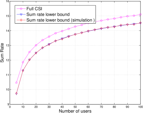
where $r_{th,j,1},r_{th,j,2},\cdots,r_{th,j,2^{b_{j}}+1}$ are the quantization levels in rank region $j$, with $r_{th,j,1}=r_{th,j}$, $r_{th,j,2^{b_{j}}+1}=r_{th,j-1}$. Fig. 6 shows that the analytical lower bound of the sum rate (31) almost matches the simulation result when $B=(0,0,0,3)$. Thus, the bound (31) is very tight.

We now discuss how to allocate available bits to quantize each region to achieve the maximum sum rate. Because all users have the same probability ${\frac{1}{K}}$ of inferring itself as being ranked the $j$th, $j=1,2,\cdots,N$, on each beam direction, the expected number of feedback bits required in addition to the rank bits is $\sum_{j=1}^{N}\frac{b_{j}}{K}$. Dropping the constant, the bit allocation problem of $N$ regions for a given beam $m$ becomes

$$\max_{{\mathbf{B}}}R_{q}({\mathbf{B}})~{}~{}~{}~{}~{}~{}~{}~{}~{}~{}~{}~{}~{}~{}~{}~{}~{}~{}~{}~{}~{}~{}~{}$$

$${\text{s.t.}\sum_{j=1}^{N}b_{j}=B_{Q},\ b_{j}\in\mathbb{Z}_{+}}.$$ (32)

Figure 6: Sum rate comparison between the mathematical lower bound and the simulation result with $B=(0,0,0,3)$, $\rho=10$ dB.

IV-A Optimal Bit Allocation

The problem (32) can be solved by the greedy algorithm, which is to assign one bit at a time to the region that will result in the maximum sum rate, because adding one more bit to any of the regions will increase the average feedback load by the same amount.

For the $s$-th single bit assigning iteration, the sum rate difference between using $b_{l,s-1}$ bits and $b_{l,s-1}+1$ bits for region $l$ can be expressed as

$$\bigtriangleup{R^{l}}(s)=R_{b_{l,s-1}+1}^{l}-R_{b_{l,s-1}}^{l},l=1,2,\ldots,N,$$ (33)

where $b_{l,s-1}$ is the number of bits for quantizing region $l$, resulting from the $(s-1)$th bit assigning iteration. $R_{m}^{l}$ is the sum rate of region $l$ using $m$ quantization bits, and can be approximated by $M_{t}\sum_{j=1}^{2^{m}}\int_{r_{th,l,j}}^{r_{th,l,j+1}}\log\left({1+r_{th,l,j}}\right)f_{X_{(1)}^{K}}(x)dx$. The region which gives the maximum sum rate increment with one additional bit will be assigned one more bit at the $s$-th iteration. The algorithm iterates until all the available quantization bits are allocated, i.e., when $s=B_{Q}$. The greedy algorithm is summarized in Table I.

TABLE I: The greedy algorithm for bit allocation.

Initialize $b_{l}=0$, $l=1,2,\ldots,N.$

For (s = 1 to $B_{Q}$)

$l=\displaystyle{arg\max_{t=1,2,\ldots,N}}\bigtriangleup{R^{t}}(s)$

$b_{l}=b_{l}+1$

End

IV-B Fast Bit Allocation Method

The sum rate formula (31) is difficult to compute. We alternatively consider minimizing the mean square quantization error as a suboptimal but simple solution. The conditional PDF of the SNR in region $j$ for a given beam $m$ is

$$f_{X_{m,k}}(x~{}|~{}r_{th,j}\leq x<r_{th,j-1})=\frac{f_{X_{m,k}}(x)}{P\left(r_{th,j}\leq x<r_{th,j-1}\right)}=\frac{K}{\rho}e^{-\frac{x}{\rho}},\ \ r_{th,j}\leq x<r_{th,j-1}.$$ (34)

The SNR variance in region $j$ can be expressed as

$$\sigma_{x,j}^{2}=\left(\begin{array}[]{c}{\displaystyle\int_{r_{th,j}}^{r_{th,j-1}}{\displaystyle x^{2}\frac{K}{\rho}e^{-\frac{x}{\rho}}}dx}\\ \end{array}\right)-\left(\begin{array}[]{c}{\displaystyle\int_{r_{th,j}}^{r_{th,j-1}}{\displaystyle x\frac{K}{\rho}e^{-\frac{x}{\rho}}}dx}\\ \end{array}\right)^{2}.$$ (37)

Thus, the variance of the quantization error using $b_{j}$ bits can be bounded by [18]

$$\sigma_{e,j}^{2}\leq\epsilon^{2}\frac{\sigma_{x,j}^{2}}{2^{b_{j}}},$$ (38)

where the constant $\epsilon$ is source dependent. For example, $\epsilon=1.0$ for uniform distributed sources and $\epsilon=2.17$ for Gaussian sources. In our case, the SNR PDFs for different regions are different, thus the $\epsilon$ that gives the tightest bound (38) will be different for different regions. In order to simplify the computation, we set the same $\epsilon$ for all regions such that the upper bound (38) is always valid. Note that this simplification is reasonable when $K$ is large such that the SNR distribution is almost uniform in all regions. We further relax the constraint for the number of quantization bits in (32) from being a positive integer to being a positive real number. Then, a new bit allocation problem based on minimizing the upper bound of the variance of the quantization error can be formulated as

$$\min_{\mathbf{B}=(b_{1},\ldots,b_{N})}\sum_{j=1}^{N}\frac{\sigma_{x,j}^{2}}{2^{b_{j}}}$$

$${{\text{s.t.}}\left\{\begin{array}[]{ll}\sum_{j=1}^{N}b_{j}=B_{Q}\\ {0\leq b_{j}\leq B_{Q}},&j=1,2,\ldots,N\\ b_{j}\in\mathbb{R_{+}}\end{array}\right.},$$ (42)

where in the objective function, the same constant $\epsilon$ and same probability $1/K$ for all regions are dropped for conciseness without changing the problem. Since the optimization problem (42) is convex, we can apply the Karush-Kuhn-Tucker (KKT) conditions [19] to solve it. To simplify the expression in (42), we let

$$L{({\mathbf{B}},{\lambda},{\nu_{1}},\ldots,{\nu_{N}},{\delta_{1}},\ldots,{\delta_{N}})}=f_{0}{(\mathbf{B})}+\lambda f_{1}{(\mathbf{B})}+\sum_{j=1}^{N}\nu_{j}h_{j}{(\mathbf{B})}+\sum_{j=1}^{N}\delta_{i}q_{j}{(\mathbf{B})}$$ (43)

where

$${\left\{\begin{array}[]{ll}f_{0}{(\mathbf{B})}=\sum_{j=1}^{N}\sigma_{x,j}^{2}2^{-b_{j}}\\ f_{1}{(\mathbf{B})}=\sum_{j=1}^{N}b_{j}-B_{Q}\\ h_{j}{(\mathbf{B})}=-b_{j}\\ q_{j}{(\mathbf{B})}=b_{j}-B_{Q}\end{array}\right.}.$$

Since $f_{o},f_{1},h_{j},q_{j}$ are differentiable, the KKT conditions for this problem are

$$\left\{\begin{array}[]{ll}\frac{\displaystyle\partial{L{({\mathbf{B}},{\lambda},{\nu_{1}},\ldots,{\nu_{N}},{\delta_{1}},\cdots,{\delta_{N}})}}}{\displaystyle\partial{b_{j}}}=0,&j=1,2,\ldots,N,\\ \sum_{j=1}^{N}b_{j}=B_{Q}\\ {\lambda}\neq 0\\ {\nu_{j}}h_{j}{(\mathbf{B})}=0,{\delta_{j}}q_{j}{(\mathbf{B})}=0,&j=1,2,\ldots,N,\\ {\nu_{j}}\geq 0,{\delta_{j}}\geq 0,&j=1,2,\ldots,N.\\ \end{array}\right.{}$$ (50)

From $\frac{\displaystyle\partial{L{({\mathbf{B}},{\lambda},{\nu_{1}},\cdots{\nu_{N}},{\delta_{1}},\cdots{\delta_{N}})}}}{\displaystyle\partial{b_{j}}}=0$, we have

$${\nu_{j}}=(-2\ln 2)2^{-2b_{j}}\sigma_{x,j}^{2}+{\lambda}+{\delta_{j}}.$$ (51)

Substitute (51) into the fourth condition in (50). By considering the $\{{\nu_{j}}=0,\delta_{j}=0,0<b_{j}<B_{Q}\}$, $\{{\nu_{j}}=0,\delta_{j}>0,b_{j}=B_{Q}\}$ and $\{{\nu_{j}}>0,\delta_{j}=0,b_{j}=0\}$ cases separately, and defining $W$ as

$$W={\frac{1}{N}}\left(\begin{array}[]{l}\displaystyle\sum_{j=1}^{N}T_{j}-V\\ \end{array}\right),$$ (53)

where $T_{j}=\frac{\ln((\ln 4)\sigma_{x,j}^{2})}{\ln 10}$ and $V=\frac{B_{Q}\ln 4}{\ln 10}$, $b_{j}$ can be obtained by

$$b_{j}={\left\{\begin{array}[]{cc}\displaystyle 0,&W>T_{j}\\ \displaystyle\frac{(T_{j}-W)\ln 10}{\ln 4},&T_{j}-V<W<T_{j}\\ \displaystyle B_{Q},&W<T_{j}-V.\\ \end{array}\right.}$$ (57)

The obtained $b_{j}$’s are then rounded to be nonnegative integers. Through simulation, we found that when $B_{Q}$ is sufficiently small $(B_{Q}\leq 3)$, the optimal bit allocation has the form ${\mathbf{B}}=(0,0,\cdots,0,B_{Q})$.

IV-C Feedback Load Analysis

Let $B_{R}$ be the number of feedback bits carrying the rank information and $B_{Q}$ be defined in (32). For the multi-threshold feedback scheme, the average number of feedback bits for the network when the number of users is $K$ can be expressed as

$$\overline{F}_{b}=KM_{t}\sum_{j=1}^{N}\left\{\frac{1}{K}(B_{R}+b_{j})\right\}=M_{t}(NB_{R}+B_{Q})$$ (58)

which does not increase with the number of users, and is a constant when the number of transmission beams $M_{t}$ and the number of regions $N$ are fixed. This is in contrast to the conventional feedback schemes whose total feedback load for the network increases with the number of users.

V Numerical Results

In this section, we compare different feedback schemes in terms of the sum rate and feedback load performance using simulation. The transmitter is equipped with $M_{t}=4$ antennas and there are $K$ users each having $M_{r}=4$ antennas. For the conventional feedback scheme, named ${\mathbf{Scheme\ A}}$, each user always feeds back to the BS the SNR values of the $M_{t}$ beams. A reduced feedback scheme was proposed in [20] where each user only feeds back its largest SNR value among all beams and the corresponding beam index. We refer to this scheme as ${\mathbf{Scheme\ B}}$. The feedback loads of both ${\mathbf{Scheme\ A}}$ and ${\mathbf{Scheme\ B}}$ increase with the number of users. The multi-threshold scheme we propose is referred to as ${\mathbf{Scheme\ C}}$. The single threshold feedback scheme proposed in [8] will be called ${\mathbf{Scheme\ D}}$. For that scheme, each user feeds back the SNR value of a beam direction when the SNR is greater than the threshold. In [8], the threshold is determined by the scheduling outage probability $P_{out}$ which is the probability that none of the users feeds back. In the performance comparison, we additionally introduce a slightly modified ${\mathbf{Scheme\ D}}$ based on the design philosophy proposed in this paper by setting the threshold as $r_{th,N}$ of ${\mathbf{Scheme\ C}}$, such that the $P_{out}$ of this scheme equals to the probability of rate loss event $P_{L}$ of ${\mathbf{Scheme\ C}}$ in (18). Thus, in the comparison, we will consider ${\mathbf{Scheme\ D}}$ with constant $P_{out}=10^{-1}$, $10^{-4}$, and $P_{out}=P_{L}=\left(1-\frac{N}{K}\right)^{K}$.

In the simulation, ${\mathbf{Scheme\ A}}$ and ${\mathbf{Scheme\ B}}$ use $B_{Q,A}$ and $B_{Q,B}$ bits, respectively, to optimally quantize their SNR values. ${\mathbf{Scheme\ C}}$ has $B_{Q}$ bits allocated to $N=4$ regions using the fast bit allocation method in Section IV-B. The number of regions is chosen to guarantee the sum rate loss upper bound in (19) smaller than the system tolerable sum rate loss $\bigtriangleup R_{P}(K)=0.25$ bps/Hz. Note that the bit allocation of ${\mathbf{Scheme\ C}}$ depends on the number of users. For ${\mathbf{Scheme\ D}}$, $B_{Q,D}$ bits are used to optimally quantize the region $[\mbox{threshold},\infty)$ where the threshold depends on the scheduling outage probability $P_{out}$.

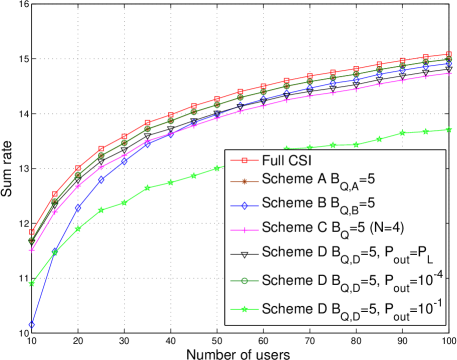
Fig. 7 compares the sum rates of different feedback schemes as the number of users increases. The numbers of SNR quantization bits defined above for different schemes are set as five. Note that for different schemes, the relationships between the number of SNR quantization bits and the total feedback load are different. Therefore, Fig. 7 is shown only to illustrate the performance difference between similar schemes. With the same number of SNR quantization bits, ${\mathbf{Scheme\ A}}$’s total feedback load is roughly four times that of ${\mathbf{Scheme\ B}}$. Thus ${\mathbf{Scheme\ A}}$’s sum rate is higher than that of ${\mathbf{Scheme\ B}}$, with the sum rate difference getting smaller as the number of users increases. This is because when the number of users is large, feeding back only the largest SNR among all beams is good enough for the purpose of scheduling. For ${\mathbf{Scheme\ D}}$, setting the threshold such that $P_{out}=10^{-4}$ results in higher sum rate compared to setting the threshold as $r_{th,4}$ when the number of users is large. This is because the scheduling outage probability of the latter increases with the number of users, and is higher than that of the former when the number of users is large. With $B_{Q}=5$, ${\mathbf{Scheme\ C}}$’s average number of feedback bits is $M_{t}(NB_{R}+B_{Q})=52$ which is less than $M_{t}NB_{Q,D}=80$ of ${\mathbf{Scheme\ D}}$ using the threshold $r_{th,4}$ (i.e., $P_{out}=P_{L}$). Thus ${\mathbf{Scheme\ C}}$’s sum rate is lower than that of ${\mathbf{Scheme\ D}}$.

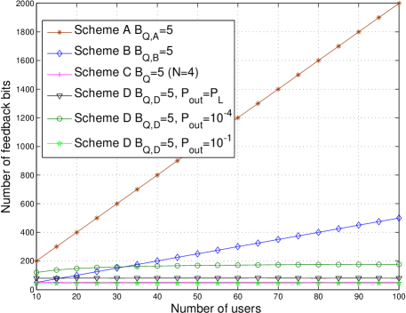
Fig. 8 shows the average total feedback loads of the cases considered in Fig. 7, and confirms the above discussion on the numbers of feedback bits for similar schemes. For example, the feedback loads of ${\mathbf{Scheme\ A}}$ and ${\mathbf{Scheme\ B}}$ grow linearly with the number of users, and the slope of ${\mathbf{Scheme\ A}}$ is four times that of ${\mathbf{Scheme\ B}}$ because ${\mathbf{Scheme\ A}}$’s users feedback the SNR of every beam. ${\mathbf{Scheme\ C}}$ and ${\mathbf{Scheme\ D}}$ with threshold $r_{th,4}$ have constant feedback loads as discussed in Section IV-C. On the other hand, ${\mathbf{Scheme\ D}}$ with constant scheduling outage probability ($P_{out}=10^{-1},10^{-4}$) has its feedback load increasing with the number of users, but saturating when the number of users is high. This is because when $P_{out}$ is fixed, ${\mathbf{Scheme\ D}}$’s threshold is $-\rho\ln(1-P_{out}^{1/K})$. When the number of users is large, ${\mathbf{Scheme\ D}}$’s feedback load is $\lim_{K\rightarrow\infty}M_{t}B_{Q}K\left(1-P_{out}^{1/K}\right)=M_{t}B_{Q}\ln(1/P_{out})$. Thus the feedback load behaviors of the three ${\mathbf{Scheme\ D}}$s are similar when the number of users is large.

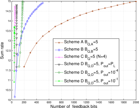
For fair comparison between the feedback schemes, the results of Fig. 7 and Fig. 8 are combined to show the sum rate as a function of the feedback load in Fig. 9. That is, the sum rate of each simulation case in Fig. 7 and its corresponding feedback load in Fig. 8 form a data point in Fig. 9. As shown in Fig. 9, for ${\mathbf{Scheme\ A}}$ and ${\mathbf{Scheme\ B}}$, the feedback load has to be increased if higher sum rate is desired. ${\mathbf{Scheme\ C}}$ and ${\mathbf{Scheme\ D}}$ with $r_{th,4}$ as the threshold ($P_{out}=P_{L}$), which is based on the same design philosophy as ${\mathbf{Scheme\ C}}$, have much lower and fixed feedback loads as their sum rates grow like $(1-e^{-N})M_{t}\log\log(K)$. It can be seen that, to achieve the same sum rate, ${\mathbf{Scheme\ C}}$ requires lower feedback load than ${\mathbf{Scheme\ D}}$. Note that, based on the design philosophy in [8], ${\mathbf{Scheme\ D}}$ with constant scheduling outage probability behaves similarly as ${\mathbf{Scheme\ A}}$ and ${\mathbf{Scheme\ B}}$. In fact, if the scheduling outage probability is set to zero, ${\mathbf{Scheme\ D}}$ will become exactly the same as ${\mathbf{Scheme\ A}}$. When ${\mathbf{Scheme\ D}}$’s $P_{out}$ is large, its sum rate loss is also large.

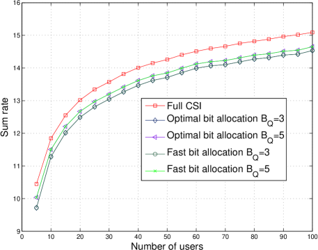
Fig. 10 compares the sum rate performance of ${\mathbf{Scheme\ C}}$ using the optimal and fast bit allocation methods discussed in Section IV. It is shown that the sum rate performances for these two bit allocation methods are visually indistinguishable. Thus, the fast bit allocation method is preferred for all practical purposes.

Figure 7: Sum rate performance comparison for different feedback schemes. $\rho=10$ dB.

Figure 8: Feedback load comparison for different feedback schemes. $\rho$=10dB.

Figure 9: Sum rate as a function of the feedback load. $\rho=10$ dB.

Figure 10: Sum rate performance comparison for different bit allocation methods in Scheme C with $N=4$ regions, $\rho=10$ dB.

VI Conclusion

In this paper, we proposed a multi-threshold feedback scheme for the MIMO broadcast channel to reduce the aggregate feedback load. The minimum number of regions (thresholds) required for a given tolerable sum rate loss was found, and the upper and lower bounds for the increment of sum rate with every additional region were derived. The multiuser diversity using the multi-threshold scheme was also investigated. Finally, the optimal bit allocation and a fast bit allocation algorithm for the multi-threshold scheme were discussed. Analytical and simulation results showed that the proposed multi-threshold feedback scheme can reduce the feedback load and utilize the limited feedback bandwidth more effectively than the existing feedback methods. In particular, while keeping the aggregate feedback load of the entire system constant regardless of the number of users, the proposed scheme almost achieves the optimal asymptotic sum rate scaling with respect to the number of users (i.e., the multiuser diversity).

References

- [1] G. Caire and S. Shamai, “On the achievable throughput for a multi-antenna Gaussian broadcast channel,” IEEE Trans. on Inf. Theory, vol. 49, no. 7, July 2003.
- [2] M. H. M. Costa, “Writing on dirty paper,” IEEE Trans. on Inf. Theory, vol. 29, no. 3, pp. 439–441, May. 1983.
- [3] H. Weingarten, Y. Steinberg, and S. Shamai, “The capacity region of the Gaussian multiple-input multiple-output broadcast channel,” IEEE Trans. on Inf. Theory, vol. 52, no. 9, pp. 3936 – 3964, Sept. 2006.
- [4] T. Yoo and A. Goldsmith, “On the optimality of multiantenna broadcast scheduling using zero-forcing beamforming,” IEEE J. Select. Areas Commun, vol. 24, pp. 528–541, Mar. 2006.
- [5] N. Jindal, “MIMO Broadcast Channels With Finite-Rate Feedback,” IEEE Trans. on Inf. Theory, vol. 52, no. 11, pp. 5045–5060, 2006.
- [6] T. Yoo, N. Jindal, and A. Goldsmith, “Multi-Antenna Downlink Channels with Limited Feedback and User Selection,” IEEE J. Select. Areas Commun, vol. 25, no. 7, pp. 1478–1491, Sep. 2007.
- [7] M. Sharif and B. Hassibi, “On the capacity of MIMO broadcast channel with partial side information,” IEEE Trans. on Inf. Theory, vol. 51, no. 2, pp. 506–522, Feb. 2005.
- [8] D. Gesbert and M. S. Alouini, “How much feedback is multi-user diversity really worth?,” IEEE Int. Conf. on Commun.(ICC), vol. 1, pp. 234–238, June 2004.
- [9] V. Hassel, M. S. Alouini, D. Gesbert, and G. E. Oien, “Exploiting multiuser diversity using multiple feedback thresholds,” IEEE VTC, vol. 2, pp. 1302–1306, May. 2005.
- [10] R. Zakhour and D. Gesbert, “A Two-Stage Approach to Feedback Design in Multi-User MIMO Channels with Limited Channel State Information,” IEEE PIMRC, vol. 24, pp. 1–5, Sep. 2007.
- [11] T. L. Marzetta and B. M. Hochwald, “Capacity of a mobile multiple-antenna communication link in Rayleigh flat fading,” IEEE Trans. on Inf. Theory, vol. 45, pp. 139–157, 1999.
- [12] J.-H. Li and H.-J. Su, “Feedback Reduction for MIMO Broadcast Channel with Heterogeneous Fading,” available: http://arxiv.org/abs/1103.3292.
- [13] D. A. Gore, R. W. Heath, and A. J. Paulraj, “Transmit Selection in Spatial Multiplexing Systems,” IEEE Communication Letter, vol. 6, pp. 491–493, Nov. 2002.
- [14] S. Ghahramani, Fundamentals of probability with stochastic processes, prentice-Hall, third edition, 2005.
- [15] O. Gascuel and G. Caraux, “Bounds on expectations of order statistics via extremal dependences,” Statist.Probab. Lett., pp. 143–148, 1992.
- [16] D.K. Sharma, “Design of Absolutely Optimal Quantizers for a Wide Class of Distortion Measure,” IEEE Trans. on Inf. Theory, vol. 24, no. 6, pp. 693–702, Nov. 1978.
- [17] C. Anton-Haro, “Optimal Quantization Schemes for Orthogonal Random Beamforming-A Cross-Layer Approach,” ICASSP, vol. 3, pp. 637–640, April. 2007.
- [18] H. H. Hang and J. J. Chen, “Source Model for Transform Video Coder and Its ApplicationPart I: Fundamental Theory,” IEEE Trans. on Circuits and Systems for Video Technology, vol. 7, no. 2, pp. 287–298, April. 1997.
- [19] S. Boyd and L. Vandenberghe, Convex Optimization, Cambridge University Press, 2004.
- [20] M. Pugh and B. D. Rao, “Reduce Feedback Schemes Using Random Beamforming in MIMO Broadcast Channels,” IEEE Trans. on Signal Processing, vol. 58, no. 3, pp. 4362–4372, March. 2010.