Spherical collapse of inhomogeneous dust cloud in the Lovelock theory

Abstract

We study gravitational collapse of a spherically symmetric inhomogeneous dust cloud in the Lovelock theory without cosmological constant. We show that the final fate of gravitational collapse in this theory depends on the spacetime dimensions. In odd dimensions the naked singularities formed are found to be massive. In the even dimensions, on the other hand, the naked singularities are found to be massless. We also show that the curvature strength of naked singularity is independent of the spacetime dimensions in odd dimensions. However, it depends on the spacetime dimensions in even dimension.

I Introduction

Whether gravitational collapse results in a black hole or a naked singularity is one of the crucial issues in classical general relativity. A singularity is not a “point” in the spacetime and information from such a place is in fact an end of causality in the theory. In order to avoid such a breakdown of physics, it is often believed that naked singularities cannot be formed under physically reasonable conditions in classical general relativity (GR). This is known as the cosmic censorship conjecture (CCC) Penrose:1969pc . Broadly there are two versions of the CCC, i.e., a strong cosmic censorship conjecture (SCCC) and a weak cosmic censorship conjecture (WCCC). The SCCC prohibits the formation of locally naked singularity, i.e., singularities are not visible to even nearby observers. On the other hand, the WCCC prohibits the formation of globally naked singularity, allowing a local observer moving around singularity to see it. Though there have been many efforts to prove the CCC, it remains as one of the important unsolved problem in GR. Meanwhile, a considerable number of counterexamples have been found violating both the WCCC and SCCC.

In 1939 Oppenheimer and Snyder studied the gravitational collapse of a spherically symmetric homogeneous dust cloud and found that the collapse ends in a black hole Oppenheimer:1939ue . However, in absence of a general proof of the CCC there have been studies on collapse using various matter models like dust, radiation, scalar fields, and so on. In these exact solutions of Einstein equations several counterexamples to the CCC have been found. For example, naked singularities form in the collapse of spherically symmetric inhomogeneous dust models Yodzis:1973 ; Eardley:1978tr ; Christodoulou:1984mz ; Newman:1985gt ; Joshi:1993zg ; Singh:1994tb ; Jhingan:1996jb (see Ref. Joshi:2008zz and the references therein). In general there are two types of singularities in spherical collapse, namely, shell-crossing and shell-focusing singularities. But, in what follows, we will focus only on the central shell-focusing singularities.

Recently, higher-dimensional spacetimes have generated considerable interest in theoretical physics. These higher-dimensional models are motivated by string/M theory. The case of collapse of a inhomogeneous dust cloud in the simple extension of GR to higher dimensions was well studied. It was shown there that the singularity cannot be naked when the spacetime dimension is more than six for smooth initial data Ghosh:2001fb ; Goswami:2004gy ; Goswami:2006ph (see also Ref. Joshi:2008zz and the references therein). More precisely, one could confirm that the SCCC holds in dimensions higher than six in such a naive extension of GR to higher dimensions. Clearly, the spacetime dimensions play an important role in the final fate of the gravitational collapse. However, it is expected that spacetime should be extremely curved near singularities putting in doubt the validity of classical GR in these regions. Indeed the string/M theory predicts the higher curvature corrections to the Einstein equation in its low-energy limit. In view of the above facts it is important to study gravitational collapse in such a theory. Though the CCC was originally formulated for general relativity, it is worthwhile to investigate the implications of stringy effects on it. In this paper, we shall address this issue while focusing on the gravitational collapse of spherical symmetric dust clouds. But there is no canonical recipe to include higher-order curvature corrections to GR. Although string theory predicts such corrections, we do not have a clear picture yet. In this paper we shall adopt a special combination of higher curvature corrections so that the field equations do not include the higher derivative terms of the metric than the third order, that is, the Lovelock theory Lovelock:1971yv . There is no strong reason why the CCC should hold in the Lovelock theory, since energy conditions are generally violated in this theory. Nevertheless, if singularities do form in this theory, it is important to know their features.

In the Lovelock theory the static black hole solutions of a spherically symmetric vacuum were found in Refs. Wheeler:1985qd ; Cai:2003kt ; Cai:2001dz . In Ref. Takahashi:2010ye ; Takahashi:2010gz the stability of a static vacuum black hole solution was discussed. The gravitational collapse of a spherical homogeneous dust cloud was analyzed in the dimensionally continued gravity Ilha:1996tc ; Ilha:1999yn (the restricted class of the Lovelock theory Banados:1993ur ). It was shown there that the singularity will be covered by event horizon as in the Oppenheimer-Snyder’s case Oppenheimer:1939ue . Subsequently, the gravitational spherical collapse of inhomogeneous dust cloud in the Gauss-Bonnet theory of gravity was addressed in Ref. Maeda:2006pm and it was shown that the final fate of collapse depends on the dimensions of spacetime. An exact solution and complete analysis in the 5-D Gauss-Bonnet theory was given in Ref. JhinganGhosh . In five dimensions, singularities were found to be naked and massive. From six to nine dimensions, singularities are naked and massless. In dimensions higher than ten, singularities are always covered. Therefore, including the Gauss-Bonnet corrections to GR makes the final state of collapse rather nontrivial. The gravitational collapse of null dust fluid was also studied Maeda:2005ci ; Nozawa:2005uy ; Dehghani:2008yc . These works also showed that the Lovelock corrections modify the collapse scenario in a nontrivial way.

In this paper we investigate the gravitational collapse of a spherical inhomogeneous dust cloud in the Lovelock gravity, without cosmological constant and in any dimensions. We show that singularities do form in the final stage of gravitational collapse in general and that they could be naked for some initial dates. Comparing with the Gauss-Bonnet gravity, we found that the Lovelock term changes the nature of singularities. In the Gauss-Bonnet case, singularities which appear in more than six dimensions are massless. In the Lovelock theory with odd dimensions, we see that singularities are massive. On the other hand, singularities are massless in the even dimensions. This is an unique feature of the Lovelock gravity.

The rest of this paper is organized as follows. In Sec. II, we briefly review the Lovelock theory. In Sec. III, we derive the basic equations for gravitational spherical dust collapse in the Lovelock theory. In Sec. IV, we analyze the nature of the singularity and apparent horizon. In Sec. V, we show the existence of null geodesics from the singularities. In Sec. VI, we analyze the strength of the naked singularities. Finally we will give our conclusion and discussion in Sec. VII. In the Appendix A, we discussed the junction between inner and outer solutions. In the Appendix B, the analysis of the homogeneous case will be briefly given. In this paper, we employ the units of $c=1$ and $8\pi G=1$, where $c$ is the speed of light and $G$ is the gravitational constant in higher dimensions.

II Lovelock theory

In this section we give an overview of the Lovelock theory in $D=n+2$-dimensional spacetimes. This is the most general theory of gravity satisfying following three conditions:

1. The field equations are written in terms of a symmetric rank-2 tensor.

2. The theory is consistent with the conservation law of the energy-momentum tensor.

3. The theory does not include higher than third order derivatives.

The Lagrangian of the theory is given by

$$\mathcal{L}=\sum_{m=1}^{k}\frac{a_{m}}{m}\mathcal{L}_{m},$$ (1)

where

$$\mathcal{L}_{m}=\frac{1}{2^{m}}\delta_{\mu_{1}\mu_{2}\dots\mu_{2m-1}\mu_{2m}}^{\nu_{1}\nu_{2}\dots\nu_{2m-1}\nu_{2m}}R_{\nu_{1}\nu_{2}}{}^{\mu_{1}\mu_{2}}\dots R_{\nu_{2m-1}\nu_{2m}}{}^{\mu_{2m-1}\mu_{2m}}{}.$$ (2)

In the above, $R_{\mu\nu}{}^{\rho\sigma}$ is the Riemann curvature tensor, and $\delta_{\mu_{1}\mu_{2}\dots\mu_{2m-1}\mu_{2m}}^{\nu_{1}\nu_{2}\dots\nu_{2m-1}\nu_{2m}}$ is the generalized and totally antisymmetric Kronecker delta. $\{a_{m}\}$ are arbitrary constants which cannot be determined by the theory itself. The suffixes $\mu_{1}\dots\mu_{2m}$ and $\nu_{1}\dots\nu_{2m}$ run from $1$ to $D$, and $k$ is a constant depending on the spacetime dimensions, defined by $k=[(D-1)/2]$ ($[x]$ is the integer part of $x$). Throughout this paper we suppose that $a_{m}$ are positive.

The field equations for this Lagrangian are

$$\mathcal{G}_{\mu}^{\nu} = -\sum_{m=1}^{k}\frac{1}{2^{m+1}}\frac{a_{m}}{m}\delta_{\mu\mu_{1}\mu_{2}\dots\mu_{2m-1}\mu_{2m}}^{\nu\nu_{1}\nu_{2}\dots\nu_{2m-1}\nu_{2m}}$$ (3)

$$\times R_{\nu_{1}\nu_{2}}{}^{\mu_{1}\mu_{2}}\dots R_{\nu_{2m-1}\nu_{2m}}{}^{\mu_{2m-1}\mu_{2m}}$$

$$= T_{\mu}^{\nu},$$

where $T^{\nu}_{\mu}$ is energy-momentum tensor of matter. It should be remembered that $\nabla^{\mu}\mathcal{G}_{\mu}^{\nu}=0$ holds, where $\nabla_{\mu}$ is the covariant derivative with respect to the metric $g_{\mu\nu}$.

There is an exact solution of the vacuum, static and spherical symmetric black hole Wheeler:1985qd ; Cai:2003kt ; Cai:2001dz . The metric is given by

$$ds^{2}=-f(r)dt^{2}+\frac{1}{f(r)}dr^{2}+r^{2}\gamma_{ij}dx^{i}dx^{j},$$ (4)

where $\gamma_{ij}$ is the line element of $n$-dimensional constant curvature hypersurface and $f(r)$ is

$$f(r)=\kappa-r^{2}\psi(r).$$ (5)

In the above, $\kappa$ is the constant curvature of the $n$-dimensional hypersurfaces which take values $-1,0\text{\ and\ }1$. In this paper we are interested only in asymptotically flat, spherically symmetric spacetime and then set $\kappa=1$. The function $\psi(r)$ is a solution to the algebraic equation

$$W[\psi]=\sum_{m=2}^{k}\bigg{[}\frac{a_{m}}{m}\bigg{\{}\prod_{p=1}^{2m-2}(n-p)\bigg{\}}\psi^{m}\bigg{]}+\psi=\frac{\mu}{r^{n+1}}.$$ (6)

Here $\mu$ is a constant proportional to the ADM mass.

Under the assumption that all the coefficient $a_{m}$ are positive, $W[\psi]$ is a monotonically increasing function of $\psi$ when $\psi>0$. Therefore, positive $\psi$ has a unique solution to Eq. (6). When we take $r\to\infty$, the positive solution goes to zero as

$$\psi=\frac{\mu}{r^{n+1}}+\mathcal{O}(\frac{1}{r^{n+2}}).$$ (7)

From this fact and the metric form of Eq. (5), it is easy to see that the solution corresponds to an asymptotically flat spacetime. A negative $\psi$ could also be the solution. But in this case, the solution corresponds to an asymptotically anti-deSitter (AdS) spacetime. In this paper we shall consider on the positive $\psi$ solution because we are interested in asymptotically flat spacetimes.

The horizon is located at $f=0$. Then the equation for the horizon is

$$\psi=\frac{1}{r^{2}}$$ (8)

and Eq. (6) implies

$$W[\psi]=\mu\psi^{(n+1)/2}$$ (9)

at the horizon. The solution to Eq. (9) depends on spacetime dimension, $n$. In even dimensions, Eq. (9) becomes

$$-\mu\psi^{(n-1)/2}+\sum_{m=2}^{n/2}\bigg{[}\frac{a_{m}}{m}\bigg{\{}\prod_{p=1}^{2m-2}(n-p)\bigg{\}}\psi^{m-1}\bigg{]}+1=0.$$

(10)

It is easy to see that there are always solutions to Eq. (10). In odd dimensions, on the other hand, Eq. (9) becomes

$$\Bigl{(}\frac{2a_{\frac{n+1}{2}}}{n+1}\bigg{\{}\prod_{p=1}^{n-1}(n-p)\bigg{\}}-\mu\Bigr{)}\psi^{(n-1)/2}$$

$$+\sum_{m=2}^{(n-1)/2}\bigg{[}\frac{a_{m}}{m}\bigg{\{}\prod_{p=1}^{2m-2}(n-p)\bigg{\}}\psi^{m-1}\bigg{]}+1=0.$$ (11)

There are the solutions to the equation above if

$$\frac{2a_{\frac{n+1}{2}}}{n+1}\bigg{\{}\prod_{p=1}^{n-1}(n-p)\bigg{\}}-\mu<0$$ (12)

is satisfied. In odd dimensions, there is a tendency that spacetimes with small mass have no horizons. This is the characteristic feature which is different from even-dimensional cases. For example, in the five-dimensional asymptotically flat solution, $f(r)$ becomes

$$f(r)=1+\frac{r^{2}}{2a_{2}}\left(1-\sqrt{1+\frac{4a_{2}\mu}{r^{4}}}\right).$$ (13)

The the event horizon is given by

$$r=\sqrt{\mu-a_{2}}.$$ (14)

Since $a_{2}>0$, the size of the Gauss-Bonnet black hole is smaller than that of the corresponding five-dimensional Schwarzschild black hole. Therefore, the Gauss-Bonnet correction weaken the gravity. Note that this solution has the naked singularity when $\mu\leq a_{2}$.

For our current study, the vacuum exact solution mentioned above stands for the outer region of the collapsing dust cloud. Actually, we can join this outer solution with the inner cloud solution (see the appendix A for the details).

III Spherical collapse of dust clouds

In this section, we will consider the spherical collapse of dust clouds in the Lovelock theory. We first write down the basic equations.

The energy-momentum tensor of dust cloud is

$$T_{\nu}^{\mu}=\varepsilon(t,r)u_{\nu}u^{\mu},$$ (15)

where $\varepsilon(t,r)$ is the energy density, which is supposed to be positive, and $u^{\mu}$ is the velocity. The metric is

$$ds^{2}=-B(t,r)^{2}dt^{2}+A(t,r)^{2}dr^{2}+R(t,r)^{2}d\Omega_{n}^{2}.$$ (16)

Here $A(t,r)$, $B(t,r)$ and $R(t,r)$ are arbitrary functions of $t$ and $r$, and $d\Omega_{n}^{2}$ is the line element of the $n$-dimensional unit sphere. Using the gauge freedom of coordinate $r$, we can always set $R(0,r)=r$. In the current paper, we assume $\partial_{t}R<0$ at initial surface. This means that the dust cloud is initially collapsing.

From the conservation equation of the energy-momentum tensor

$$\nabla_{\nu}T^{\nu}_{\mu}=0,$$ (17)

we have two equations

$$\varepsilon\frac{B^{\prime}}{B} =0,$$ (18)

$$\dot{\varepsilon}+\varepsilon\left(\frac{\dot{A}}{A}+n\frac{\dot{R}}{R}\right) =0.$$ (19)

In the above the dot and prime denote the partial derivative of $t$ and $r$, respectively.

It is easy to see that Eq. (18) implies $B=B(t)$. Then, without a loss of generality, we can set $B=1$. Now the metric becomes

$$ds^{2}=-dt^{2}+A(t,r)^{2}dr^{2}+R(t,r)^{2}d\Omega_{n}^{2}\,,$$ (20)

and the gravitational field equations for this simplified metric are

$$\sum_{m=1}^{k}a_{m}\prod_{p=0}^{2m-2}(n-p)\left(\left(\frac{\dot{R}}{R}\right)^{2}-\left(\frac{R^{\prime}}{RA}\right)^{2}+\frac{1}{R^{2}}\right)^{m-1}\left(\frac{\ddot{R}}{R}+\frac{\left(n-\left(2m-1\right)\right)}{2m}\left(\left(\frac{\dot{R}}{R}\right)^{2}-\left(\frac{R^{\prime}}{RA}\right)^{2}+\frac{1}{R^{2}}\right)\right)=0,$$ (21)

$$\sum_{m=1}^{k}a_{m}\prod_{p=0}^{2m-2}(n-p)\left(\left(\frac{\dot{R}}{R}\right)^{2}-\left(\frac{R^{\prime}}{RA}\right)^{2}+\frac{1}{R^{2}}\right)^{m-1}$$

$$\times\Biggl{(}-\frac{R^{\prime\prime}}{RA^{2}}+\frac{R^{\prime}A^{\prime}}{RA^{3}}+\frac{\dot{R}\dot{A}}{RA}+\frac{\left(n-\left(2m-1\right)\right)}{2m}\Bigl{(}\left(\frac{\dot{R}}{R}\right)^{2}-\left(\frac{R^{\prime}}{RA}\right)^{2}+\frac{1}{R^{2}}\Bigl{)}\Biggr{)}=\varepsilon(t,r),$$ (22)

and

$$\sum_{m=1}^{k}a_{m}\prod_{p=0}^{2m-2}(n-p)\left(\left(\frac{\dot{R}}{R}\right)^{2}-\left(\frac{R^{\prime}}{RA}\right)^{2}+\frac{1}{R^{2}}\right)^{m-1}\left(\frac{\dot{R}^{\prime}}{RA^{2}}-\frac{R^{\prime}\dot{A}}{RA^{3}}\right)=0.$$ (23)

From Eq. (23), we see that

$$\frac{\dot{R}^{\prime}}{RA^{2}}-\frac{R^{\prime}\dot{A}}{RA^{3}}=0$$ (24)

holds. This equation can be easily integrated as

$$A=\frac{R^{\prime}}{W(r)},$$ (25)

where $W(r)$ is the arbitrary function of $r$. Introducing $L$ by

$$L\equiv\sum_{m=1}^{k}\frac{a_{m}}{2m}\prod_{p=0}^{2m-2}(n-p)\left(\dot{R}^{2}+1-W^{2}\right)^{m}\frac{1}{R^{2m}},$$ (26)

and using Eq. (25), we can rewrite Eqs. (21) and (22) in the following simple forms

$$\frac{1}{\dot{R}R^{n}}\frac{\partial}{\partial t}\left(LR^{n+1}\right) =0,$$ (27)

$$\frac{1}{R^{\prime}R^{n}}\frac{\partial}{\partial r}\left(LR^{n+1}\right) =\varepsilon(t,r).$$ (28)

Then the integration of the above equations implies

$$L=\frac{n}{2}\frac{F(r)}{R^{n+1}},$$ (29)

where $F(r)$ is a function of $r$, which can be interpreted as a sort of mass function defined as

$$F(r)=\frac{2}{n}\int_{0}^{r}\varepsilon R^{n}R^{\prime}dr.$$ (30)

Indeed, $F(r)$ is proportional to the generalized Misner-Sharp mass Maeda:2011ii . Using $F(r)$, Eq. (28) can be reexpressed as

$$\varepsilon=\frac{n}{2}\frac{F(r)^{\prime}}{R^{n}R^{\prime}}.$$ (31)

For later convenience, we shall introduce the coefficients $c_{l}$ by

$$c_{l}=\begin{cases}1&\text{if}\ \ l=1\\ \frac{a_{l}}{l}\prod_{p=1}^{2l-2}(n-p)&\text{if}\ \ 2\leq l\leq k.\end{cases}$$ (32)

Using this, Eq. (29) becomes

$$\sum_{m=1}^{k}c_{m}\left(\dot{R}^{2}+1-W^{2}\right)^{m}\frac{1}{R^{2m}}=\frac{F(r)}{R^{n+1}}.$$ (33)

This is the key equation for the gravitational collapse.

From Eq. (31), we can see two types of singularities which correspond to blowing up of energy density, that is, the shell-focusing singularities which form at at $R=0$, and the shell-crossing singularities at $R^{\prime}=0$. In this paper we assume $R^{\prime}>0$ to exclude the shell-crossing singularities from our consideration.

To make the initial surface regular at the center ($r=0$), the function $F(r)$ should behave as

$$F(r)=r^{n+1}M(r),$$ (34)

where $M(r)$ is some regular function on initial surface.

For later convenience, we introduce the function $v(t,r)$ through

$$R(t,r)=rv(t,r).$$ (35)

Then our current initial conditions of $R(t,r)$ are expressed as

$$v(0,r)=1,$$ (36)

$$\dot{v}(0,r)<0.$$ (37)

The singularities at $R=0$ are located at the orbit satisfying $v(t,r)=0$.

Before closing this section, we have one remark. At first glance,

$$\sum_{m=1}^{k}a_{m}\prod_{p=0}^{2m-2}(n-p)\left(\left(\frac{\dot{R}}{R}\right)^{2}-\left(\frac{R^{\prime}}{RA}\right)^{2}+\frac{1}{R^{2}}\right)^{m-1}=0$$ (38)

is also the solution to Eq. (23). Combining above with Eq. (21), we have

$$\sum_{m=1}^{k}a_{m}\prod_{p=0}^{2m-2}(n-p)\frac{\left(n-\left(2m-1\right)\right)}{2m}$$

$$~{}~{}\times\left(\left(\frac{\dot{R}}{R}\right)^{2}-\left(\frac{R^{\prime}}{RA}\right)^{2}+\frac{1}{R^{2}}\right)^{m}=0.$$ (39)

Together with Eq. (22), we can show that this implies $\varepsilon(t,r)=0$. This means that the spacetimes must be vacuum, which is a solution but not our interest here.

IV Apparent horizons and singularities

In this section we analyze the structure of spacetimes obtained in the previous section. We shall focus on the behavior of trapped surfaces and apparent horizons surrounding the singularities.

We shall investigate the even and odd-dimensional cases separately since it is clear from Eqs. (10) and (11) that they should have quite different features. As stated in Sec. II, we assume that all coefficients $c_{l}$ are positive. Here we also take $W(r)=1$, which corresponds to the “marginally bound case”.

First of all, it should be noted that bounce ($\dot{v}=0$ and $v\neq 0$) cannot occur in this case for initially collapsing configurations. Then we will be able to expect the appearance of the shell-focusing singularity in general. Using Eqs. (34) and (35), Eq. (33) becomes

$$\sum_{m=1}^{k}c_{m}\left(\frac{\dot{v}}{v}\right)^{2m}=\frac{M(r)}{v^{n+1}}.$$ (40)

Substituting $\dot{v}=0$ into Eq. (40), then we have

$$M(r)=0$$ (41)

for the bounce. This contradicts our assumption that $\varepsilon$ is positive. From this fact, bounce cannot occur and the cloud continues to collapse. We can also see from this that the range of $v$ is from $0$ to $1$.

A trapped surface is described by the surfaces which satisfy $dR/dt|_{\pm}<0$, where $d/dt|_{+}$ and $d/dt|_{-}$ are derivatives along the outgoing and ingoing null geodesics respectively. For the current metric form, $dR/dt|_{\pm}$ becomes

$$\frac{dR}{dt}\bigg{|}_{+} =\dot{R}+\frac{dr}{dt}\bigg{|}_{+}R^{\prime}=\dot{R}+1,$$ (42)

$$\frac{dR}{dt}\bigg{|}_{-} =\dot{R}+\frac{dr}{dt}\bigg{|}_{-}R^{\prime}=\dot{R}-1,$$ (43)

where we used the fact of $dr/dt|_{\pm}=\pm R^{\prime-1}$. The apparent horizon is defined to be the boundary of trapped regions. In our case it is easy to see that the location of the apparent horizons can be found through the solving of

$$g^{\mu\nu}R_{,\mu}R_{,\nu}=0.$$ (44)

For the metric of Eq. (20), this condition becomes

$${\dot{R}^{2}}=1.$$ (45)

IV.1 Even dimensions

We first consider the apparent horizon in even dimensions. Using Eq. (45), Eq. (33) implies

$$H_{even}(R)\equiv\sum_{m=1}^{k=n/2}c_{m}R^{n-2m+1}=F(r)\,,$$ (46)

which determines the location of the apparent horizons. Note that the left-hand side of the equation above is an odd function of $R,$ and $F(r)$ is a monotonically increasing function of $r,$ with $\lim_{r\to 0}F(r)=0$. We depict the behavior of the left-hand side of Eq. (46) in Fig. 1.

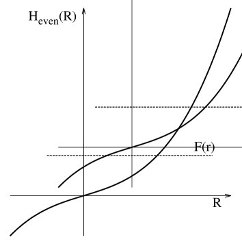
Figure 1: The profile of function $H_{even}(R)$. The thick line is $H_{even}(R)$ and the dotted line is $F(r)$. $H_{even}(R)$ is the odd function and we assume that all coefficients are positive. Therefore, $H_{even}$ is monotonically increasing function for $R>0$ and $H_{even}(0)=0$.

As shown in the figure, for any given finite $r$, we always have a solution to Eq. (46). This implies that the apparent horizons always exist in these spacetimes and all singularities which occur at finite $r>0$ (but, $R=0$) will be the inside of the apparent horizon. Therefore, only the central singularity at $r=0$ could be naked. In addition, they are massless because $F(0)=0$, in even dimensions. (Note that $F(r)$ is proportional to a quasilocal mass.) This is the same property as in the Gauss-Bonnet case. In the Gauss-Bonnet case, all singularities except for $r=0$ were found to be covered by apparent horizons in any dimensions higher than six Maeda:2006pm .

Next, let us confirm that the region inside the apparent horizon is trapped. From Eq. (33), $\dot{R}^{2}$ continues to increase during the collapse, which means $R$ decreases. This implies $\dot{R}$ is monotonically decreasing because we assume that the dust cloud is initially collapsing. Then, we can see that the region inside of the apparent horizon($\dot{R}=-1$) is actually trapped, $dR/dt|_{\pm}<0$, from Eqs. (42) and (43).

IV.2 Odd dimensions

As in even dimensional cases, Eqs. (45) and (33) give

$$H_{odd}(R)\equiv\sum_{m=1}^{k=(n+1)/2}c_{m}R^{n-2m+1}=F(r)\,,$$ (47)

which determines the location of the apparent horizons. Contrary to what we had in even dimensions, the left-hand side of Eq. (47) is the even function of $R$ (See Fig. 2).

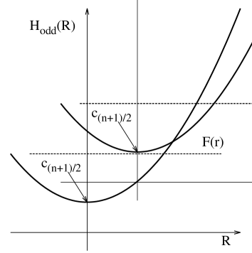
Figure 2: The profile of the function $H_{odd}(R)$. The thick line is $H_{odd}(R)$ and the dotted line is $F(r)$. $H_{odd}(R)$ is the even function and we assume that all coefficients are positive. Therefore $H_{odd}$ is monotonically increasing function of $R>0$ and $H_{odd}(0)=c_{(n+1)/2}>0$. The figure shows that $r$ satisfying $F(r)<c_{(n+1)/2}$ have no solution to Eq. (47).

In the range of $0\leq r\leq r_{ah}$, we see that there are no solutions, where $r_{ah}$ is determined through

$$F(r_{ah})=c_{(n+1)/2}.$$ (48)

Hence the singularities which occurs in the range $0\leq r\leq r_{ah}$ are not wrapped by the apparent horizons. They could be naked and massive ( $F(r^{*})\geq 0$ where $0\leq r^{*}\leq r_{ah}$) in odd dimensions. This result is in agreement with what is observed in the five-dimensional Gauss-Bonnet case Maeda:2006pm . For the Gauss-Bonnet case in any dimensions higher than six, however, the singularities at finite $r$ shall always be safely wrapped. We also see that the region inside of the apparent horizon is trapped region from the same argument in even-dimensional cases.

V Null geodesics from singularities

In this section, we shall analyze whether singularities, which are not wrapped by apparent horizons, can be naked or not. To this end we examine the existence of future-directed outgoing radial null geodesics from these singularities. Again, we need to analyze odd- and even-dimensional cases separately.

From the metric of Eq. (20), the outgoing radial null geodesic equation becomes

$$\frac{dt}{dr}=R^{\prime}.$$ (49)

To show the existence of solution for this differential equation from the singularity, we shall employ the fixed-point method Christodoulou:1984mz ; Newman:1985gt ; Maeda:2006pm . We define a new function

$$x\equiv\frac{R}{(r-r_{s})^{q}},$$ (50)

where $q$ is a positive constant and $r_{s}$ is the location of singularities. Using $x$, the null geodesic equation can be rewritten as

$$\frac{dx}{dr}+\frac{qx}{r-r_{s}}=\Xi(x,r),$$ (51)

where $\Xi(x,r)$ is given by

$$\Xi(x,r)=\frac{R^{\prime}}{(r-r_{s})^{q}}\left(1+\dot{R}\right).$$ (52)

One may consider the cases in which the function $\Xi(x,r)$ can be expanded around $r=r_{s}$

$$\Xi(x,r) \simeq \frac{g_{0}(q)x+\sum_{i=1}^{N}g_{i}(q)x^{\alpha_{i}}}{r-r_{s}}+h(q,x)(r-r_{s})^{a}$$ (53)

$$~{}~{}+o((r-r_{s})^{a}),$$

where $a$ $(>-1)$ and $\alpha_{i}\neq 1$ are constants. $g_{0},g_{i}$ and $h$ are some functions. $N\geq 1$ is an integer. We will be able to use the following useful lemma to show the existence of radial null geodesic from singularities

Lemma [Lemma 10 in Ref. Maeda:2006pm ]- If $\Xi(x,r)$ is expanded as Eq. (53) with $N=1$ and $g_{0}(q)\neq q$, there exists an asymptotic solution satisfying $x(r_{s})=[g_{1}/(q-g_{0})]^{1/(1-\alpha_{1})}$ near $r=r_{s}$, and moreover it is the unique solution to Eq. (51) which is continuous at $r=r_{s}$.

By virtue of this lemma, it is enough to investigate the features of the function $\Xi(x,r)$ for our current purpose. Hereafter we are interested in the future-directed outgoing null geodesics, which correspond to positive $x(r_{s})$, as can be seen from Eq. (49).

From now on, we will address the existence of the null geodesics in odd- and even-dimensional cases separately.

V.1 Odd dimensions

As seen in the previous section, odd-dimensional spacetimes may have complicated structures.

V.1.1 Singularities at $r_{s}=0$

We first analyze the geodesics from singularity at $r=0$ in odd dimensions. In odd dimensions, the gravitational Eq. (40) becomes

$$\sum_{m=1}^{(n+1)/2}c_{m}\left(\frac{\dot{v}}{v}\right)^{2m}=\frac{M(r)}{v^{n+1}}.$$ (54)

Solving this with respect to $\dot{v}$, we have the following formal solution

$$\dot{v}=V_{o}(v,r).$$ (55)

The formal integration of this with respect to $v$ is

$$t(v,r)=\int_{1}^{v}\frac{ds}{V_{o}(s,r)}.$$ (56)

Let us assume the smooth distribution of matter near the center($r=0$) as

$$M(r)=M_{0}+M_{2}r^{2}+M_{4}r^{4}+\dots.$$ (57)

Then $t(v,r)$ behaves near $r=0$ as

$$t(v,r)=t(v,0)+\frac{r^{2}}{2}\chi_{2}(v)+\dots.$$ (58)

The orbit of the singularities is given by $t_{s}(r)=t(0,r)$. Since the definition of $\chi_{2}(v)$ is complicated, we will not write down its explicit form. Regardless of the theory, it is shown that $\chi_{2}(0)$ is non-negative under the condition of $R^{\prime}>0$ and $\dot{R}<0$ in Ref. Maeda:2006pm . Here we further assume that $\chi_{2}(0)$ is positive, that is, $\chi_{2}(0)$ cannot achieve zero (this corresponds to the assumption for the initial data). Using the relation, which always holds,

$$0=\left(\frac{\partial t}{\partial v}\right)_{r}\left(\frac{\partial v}{\partial r}\right)_{t}+\left(\frac{\partial t}{\partial r}\right)_{v},$$ (59)

we have

$$v^{\prime}=\left(-r\chi_{2}(v)+\dots\right)\dot{v}.$$ (60)

Now we set $q=3$ in Eq. (52) and then we can expand $\Xi(x,r)$, with the help of Eqs. (54), (57) and (60), as

$$\Xi(x,r) =\left(\frac{v+rv^{\prime}}{r^{3}}\right)\left(1+r\dot{v}\right)$$

$$=\frac{x+\chi_{2}(v)\left(\frac{M_{0}}{c_{\frac{n+1}{2}}}\right)^{1/(n+1)}}{r}+\mathcal{O}(r^{0}).$$ (61)

From this expansion, the existence of solution to the null geodesic Eq. (51) with

$$x(0)=\frac{\chi_{2}(0)}{2}\left(\frac{M_{0}}{c_{\frac{n+1}{2}}}\right)^{1/(n+1)}>0$$ (62)

is guaranteed according to the lemma. Since the positivity of $x(0)$ means the null geodesic is future-directed and outgoing null, this shows that the singularities are at least locally naked.

V.1.2 Singularities at $0<r_{s}<r_{ah}$

Next let us consider the geodesics from singularities at $0<r_{s}<r_{ah}$. We consider the initial condition of

$$M(r)=\tilde{M}_{0}+\tilde{M}_{1}(r-r_{s})+\tilde{M}_{2}(r-r_{s})^{2}+\dots.$$ (63)

In the previous case of $r_{s}=0$, we assumed smoothness at the center which implies no kinklike distribution of matter. Therefore the next-to-leading term of expansion is the order of $\mathcal{O}(r^{2})$. However, $r=r_{s}\neq 0$ is not the symmetric center and then the next-to-leading term of expansion will be $\mathcal{O}(r-r_{s})$ in general.

Near the singularities, then, $t(v,r)$ behaves as

$$t(v,r)=t(v,0)+(r-r_{s})\tilde{\chi}_{1}(v)+\dots.$$ (64)

Following Ref. Maeda:2006pm , it is shown that $\tilde{\chi}_{1}(0)$ is non-negative. Here we simply assume that $\tilde{\chi}_{1}(0)$ cannot achieve zero. Using Eqs. (59) and (64), we see

$$v^{\prime}=(-\tilde{\chi}_{1}(v)+\dots)\dot{v}.$$ (65)

Setting $q=1$ in Eq. (52), we can expand $\Xi(\tilde{x},r)$, with the help of Eqs. (54), (63) and (65), as

$$\Xi(\tilde{x},r)=\frac{r_{s}}{r-r_{s}}\tilde{\chi}_{1}(v)\left(\frac{\tilde{M}_{0}}{c_{\frac{n+1}{2}}}\right)^{1/(n+1)}\left(1-r_{s}\left(\frac{\tilde{M}_{0}}{c_{\frac{n+1}{2}}}\right)^{1/(n+1)}\right)+\mathcal{O}((r-r_{s})^{0}).$$ (66)

According to Eqs. (48) and (63), $r_{ah}$ is

$$r_{ah}=\left(\frac{c_{\frac{n+1}{2}}}{\tilde{M}_{0}}\right)^{1/(n+1)}.$$ (67)

From this expansion, the existence of a solution to the null geodesic Eq. (51) from singularities at $r=r_{s}$ ($0<r_{s}<r_{ah}$) with

$$\tilde{x}(r_{s})=r_{s}\tilde{\chi}_{1}(0)\left(\frac{\tilde{M}_{0}}{c_{\frac{n+1}{2}}}\right)^{1/(n+1)}\left(1-r_{s}\left(\frac{\tilde{M}_{0}}{c_{\frac{n+1}{2}}}\right)^{1/(n+1)}\right)>0$$ (68)

is proved according to the lemma. This means that the singularities are at least locally naked.

V.2 Even dimensions

Finally we shall consider the even-dimensional spacetimes. In even dimensions the gravitation field equation of (40) becomes

$$\sum_{m=1}^{n/2}c_{m}\left(\frac{\dot{v}}{v}\right)^{2m}=\frac{M(r)}{v^{n+1}}.$$ (69)

Then we obtain formally

$$\dot{v}=V_{e}(v,r).$$ (70)

The integration of this with respect to $v$ is

$$t(v,r)=\int_{1}^{v}\frac{ds}{V_{e}(s,r)}.$$ (71)

We also consider the smooth distribution of matter as

$$M(r)=\bar{M}_{0}+\bar{M}_{2}r^{2}+\bar{M}_{4}r^{4}+\dots.$$ (72)

Then $t(v,r)$ behaves like

$$t(v,r)=t(v,0)+\bar{\chi}_{2}(v)\frac{r^{2}}{2}+\dots$$ (73)

As in the case of odd dimensions, we assume that $\bar{\chi}_{2}(0)$ is positive. According to Eq. (59), we have

$$v^{\prime}=\left(-r\bar{\chi}_{2}(v)+\dots\right)\dot{v}.$$ (74)

Setting $q=\frac{3n+1}{n+1}$ in Eq. (52), we can expand $\Xi(\bar{x},r)$, with the help of Eqs. (69), (72) and (74), as

$$\Xi(\bar{x},r)=\frac{\bar{x}+\bar{\chi}_{2}(v)\bar{x}^{-1/n}\left(\frac{\bar{M}_{0}}{c_{\frac{n}{2}}}\right)^{1/n}}{r}+\mathcal{O}(r^{-2/(n+1)}).$$ (75)

From this expansion, the existence of solution to the null geodesic Eq. (51) with

$$\bar{x}(0)=\left(\frac{n+1}{2n}\right)^{n/(n+1)}\bar{\chi}_{2}(0)^{n/(n+1)}\left(\frac{\bar{M}_{0}}{c_{\frac{n}{2}}}\right)^{1/(n+1)}>0$$ (76)

is guaranteed according to the lemma. Then the singularity is at least locally naked in this case too.

VI Strength of singularity

We finally compute the strength of naked singularity, which is the most important feature characterizing singularities. We define

$${\cal R}=R_{\mu\nu}k^{\mu}k^{\nu},$$ (77)

where $k^{\mu}=\frac{dx^{\mu}}{d\lambda}$ is the tangential vector of future out-going null geodesics from singularity and $\lambda$ is the affine parameter of the geodesics. We will check the behavior of ${\cal R}$ near the singularity (See Ref. Abdolrahimi:2009dc for a more systematic definition of the strength of singularity).

Consider the future outgoing radial null geodesics from singularities. We have a relation from the metric of Eq. (20) as follows

$$k^{t}=R^{\prime}k^{r}$$ (78)

By a straightforward calculation using Eq. (78), we have

$${\cal R}=\frac{nF(r)^{\prime}}{\sum_{m=1}^{k}2mc_{m}R^{n-2m+2}\dot{R}^{2m-2}}R^{\prime}(k^{r})^{2}.$$ (79)

The radial null geodesic equation is

$$\frac{dk^{r}}{d\lambda}+\left(\frac{R^{\prime\prime}}{R^{\prime}}+2\dot{R}^{\prime}\right)(k^{r})^{2}=0.$$ (80)

We need to consider odd- and even-dimensional cases separately.

VI.1 Odd dimensions

VI.1.1 Singularity at $r=0$

Near the singularity at $r=0$, we can compute ${\cal R}$ as

$${\cal R}\sim 3n\left(\frac{M_{0}}{c_{\frac{n+1}{2}}}\right)^{2/(n+1)}(k^{r})^{2}.$$ (81)

The geodesic equation near the singularity becomes

$$\frac{dk^{r}}{d\lambda}+\frac{2}{r}(k^{r})^{2}\simeq 0.$$ (82)

The integration of Eq. (82) gives us

$$r\sim\lambda^{1/3}.$$ (83)

We now evaluate the behavior of ${\cal R}$ near the singularities as

$${\cal R}\sim\lambda^{-\frac{4}{3}}.$$ (84)

In odd-dimensional cases, we confirmed that ${\cal R}$ diverges at $r=0$ and the behavior of divergence does not depend on the spacetime dimensions.

VI.1.2 Singularity at $0<r_{s}<r_{ah}$

Near the singularities at $r=r_{s}$, ${\cal R}$ behaves as

$${\cal R}\sim\frac{nr_{s}}{r-r_{s}}\left(\frac{\tilde{M}_{0}}{c_{\frac{n+1}{2}}}\right)^{2/(n+1)}\left(1+\frac{r_{s}}{n+1}\frac{\tilde{M}_{1}}{\tilde{M_{0}}}\right)(k^{r})^{2}.$$ (85)

The geodesic equation becomes

$$\frac{dk^{r}}{d\lambda}+C(k^{r})^{2}\simeq 0,$$ (86)

where $C$ is a constant depending on the initial data. From Eq. (86) we see that

$$r-r_{s}\sim\lambda,$$ (87)

near the singularity ($\lambda\simeq 0$). Then we can see

$${\cal R}\sim\lambda^{-1}.$$ (88)

As a result, ${\cal R}$ diverges at $r=r_{s}$ ($0<r_{s}<r_{ah}$) and the behavior of divergence does not depend on the spacetime dimensions.

VI.2 Even dimensions

VI.2.1 Singularity at $r=0$

We can evaluate ${\cal R}$ near the central singularity as

$${\cal R}\sim(3n+1)\left(\frac{\bar{M}_{0}}{\bar{x}(0)c_{\frac{n}{2}}}\right)^{2/n}\frac{(k^{r})^{2}}{r^{4/(n+1)}}.$$ (89)

The geodesic equation near the singularity is

$$\frac{dk^{r}}{d\lambda}+\frac{2n}{(n+1)r}(k^{r})^{2}\simeq 0.$$ (90)

The integration of Eq. (90) implies

$$r\sim\lambda^{\frac{n+1}{3n+1}}.$$ (91)

Thus, near singularity, we have

$${\cal R}\sim\lambda^{-4\left(\frac{n+1}{3n+1}\right)}\,.$$ (92)

In the even-dimensional cases, ${\cal R}$ diverges at $r=0$ and its behavior depends on the dimensions. This feature is different from odd-dimensional cases.

VII Summary and discussion

In this paper we considered gravitational collapse of a spherical inhomogeneous dust cloud in the Lovelock gravity with any dimension. We found that the formation of apparent horizon depends on the dimensions, that is, if it is odd or even. In even dimensions, noncentral singularities ($r\neq 0)$ will be safely wrapped by apparent horizons and only “central” singularities at $r=0$ could be naked. In odd dimensions, on the other hand, even those singularities which form at $0\leq r\leq r_{ah}$ may not be wrapped by apparent horizons and they could be naked. We also studied the future-directed outgoing null geodesics from singularities. Then we showed the existence of radial null geodesics from singularities in odd and even dimensions separately. This is a clear violation of cosmic censorship conjecture (at least the strong version). As we mentioned in the introduction, singularities cannot be naked in more than six-dimensional spacetime in the naive dimensional extension of the Einstein gravity. Therefore the Lovelock corrections worsen the situation in the aspect of the CCC. These results coincide with those of the spherical collapse of inhomogeneous dust in the Gauss-Bonnet theory, which is special case of the Lovelock theory, and the null dust collapse in the Lovelock theory.

Compared with the Gauss-Bonnet gravity, we found that the Lovelock term changes the nature of singularities more drastically. In the Gauss-Bonnet case, only massless naked singularities could form in more than six dimensions. However, we found that massive naked singularities can form in all odd dimensions in the Lovelock gravity.

We also examined the strength of the singularities and found that $R_{\mu\nu}k^{\mu}k^{\nu}$ , with the null tangent $k^{\mu}$ , diverges at the singularities for all cases considered here. We also showed that the behavior of divergence depends on the spacetime dimensions in even dimension. However, it does not depend on the spacetime dimensions in the odd case. It is a characteristic feature of the Lovelock gravity.

In this paper we had several assumptions which should be relaxed in future studies. First of all, we focused on the marginally bound cases with $W(r)=1$. But, our analysis can be easily extended to the nonmarginally bound cases $(W(r)\neq 1)$. We assumed that the matter is a dust cloud. From the standpoint of the CCC, we should deal with more generic matter fields. We also assumed here spherical symmetry. Finally, most of our work is just the local analysis of singularity. The global visibility of singularity is still unclear. These are some of the remaining issues which will be hopefully addressed in the near future.

Appendix A Junction between inner and outer solutions

In this appendix, we will address the junction between the inner and outer solutions. We suppose that the inner solution is the collapsing dust cloud presented in the main text and the outer solution is a static vacuum black hole. We follow the argument in Refs. Maeda:2006pm ; Poisson:2004 , where they discussed the similar junctions in the Gauss-Bonnet theory and Einstein theory.

Let $\Sigma$ to be the boundary of the two regions. The inner solution to Eqs. (20) and (25) is

$$ds^{2}=-dt^{2}+R^{\prime}{}^{2}dr^{2}+R^{2}d\Omega_{n}^{2},$$ (93)

and the outside solution to Eq. (4) is

$$ds^{2}=-f(R)dT^{2}+\frac{1}{f(R)}dR^{2}+R^{2}d\Omega_{n}^{2}.$$ (94)

We suppose that $\Sigma$ is described by parametric equations $R=R_{\Sigma}(t)$ and $T=T_{\Sigma}(t)$. In addition, it is natural to think that the boundary is the comoving, that is, $r=r_{0}=$constant because of dust. The induced metric on $\Sigma$ from the metric of the inner region is written as

$$ds^{2}=-dt^{2}+R_{\Sigma}^{2}d\Omega_{n}^{2}.$$ (95)

On the other hand, using the metric of the outer region is also rewritten as

$$ds^{2}=-\left(f(R_{\Sigma})\dot{T}^{2}_{\Sigma}-\frac{\dot{R_{\Sigma}}^{2}}{f(R_{\Sigma})}\right)dt^{2}+R_{\Sigma}^{2}d\Omega_{n}^{2}.$$ (96)

Of course, they should be identical and then we see that

$$1=\left(f(R_{\Sigma})\dot{T}^{2}_{\Sigma}-\frac{\dot{R_{\Sigma}}^{2}}{f(R_{\Sigma})}\right)$$ (97)

holds.

The extrinsic curvatures of $\Sigma$ evaluated from inner metric are

$${}^{-}K^{t}_{t} =0,$$ (98)

$${}^{-}K^{i}_{j} =\delta^{i}_{j}R_{\Sigma}^{-1}.$$ (99)

In terms of the metric of the outer region, the extrinsic curvatures also have another expression as

$${}^{+}K^{t}_{t} =\frac{\dot{\beta}}{\dot{R_{\Sigma}}}\left(f(R_{\Sigma})\dot{T}^{2}_{\Sigma}-\frac{\dot{R_{\Sigma}}^{2}}{f(R_{\Sigma})}\right)^{-1},$$ (100)

$${}^{+}K^{i}_{j} =\delta^{i}_{j}\frac{\beta}{R_{\Sigma}},$$ (101)

where

$$\beta=\sqrt{f+\dot{R}^{2}}=f\dot{T}.$$ (102)

The continuity of the extrinsic curvature implies us

$$\beta=1.$$ (103)

From the definition of $\beta$, we have the following two equations

$$\frac{dT_{\Sigma}}{dt} =f(R_{\Sigma})^{-1},$$ (104)

$$\left(\frac{dR_{\Sigma}}{dt}\right)^{2} =1-f(R_{\Sigma}),$$ (105)

where

$$f(R_{\Sigma})=1-R^{2}_{\Sigma}\psi(R_{\Sigma}).$$ (106)

Then we see that

$$\left(\frac{\dot{R}_{\Sigma}}{R_{\Sigma}}\right)^{2}=\psi(R_{\Sigma})$$ (107)

is required.

It is remembered that $\psi$ is the solution to Eq. (6) as in the form of

$$\sum_{m=1}^{k}c_{m}\psi^{m}=\frac{\mu}{R^{n+1}_{\Sigma}},$$ (108)

and $\dot{R}$ is the solution to Eq. (33)

$$\sum_{m=1}^{k}c_{m}\left(\frac{\dot{R}_{\Sigma}}{R_{\Sigma}}\right)^{2m}=\frac{F(r_{0})}{R^{n+1}_{\Sigma}}.$$ (109)

As seen easily, Eq. (107) is satisfied only if

$$\mu=F(r_{0}).$$ (110)

This shows that the inner region can be naturally joined to the outer region if $\mu=F(r_{0})$ is satisfied.

Appendix B Homogeneous dust collapse

In this section, we briefly discuss homogeneous case which is just a special case of inhomogeneous collapse. In this case, the spacetime metric becomes

$$ds^{2}=-dt^{2}+a^{2}(t)\big{(}dr^{2}+r^{2}d\Omega_{n}^{2}\big{)}.$$ (111)

Equation (33) reduces to

$$\sum_{m=1}^{k}c_{m}\left(\frac{\dot{a}}{a}\right)^{2m}=\frac{M}{a^{n+1}},$$ (112)

where $M$ is a constant. From this equation, we can see that the behavior of $a$ near the singularity ($a=0$) as

$$a(t)\sim (t_{s}-t)\ \$$ (in odd dimensions) (113)

$$a(t)\sim (t_{s}-t)^{n/n+1}\ \$$ (in even dimensions) (114)

where $t_{s}$ stands for the epoch of the singularity formation. From these behaviors, it turns out that singularity is ingoing-null in odd dimensions and is spacelike in even dimensions according to Ref. senovilla . In the Gauss-Bonnet homogeneous case Maeda:2006pm , singularity in five dimension is ingoing-null and is spacelike in dimensions higher than six. Therefore, as in the main text, we can confirm that the Lovelock terms changes the nature the singularity.

References

- (1) R. Penrose, Riv. Nuovo Cim. 1, 252 (1969) [Gen. Rel. Grav. 34, 1141 (2002)].
- (2) J. R. Oppenheimer and H. Snyder, Phys. Rev. 56, 455 (1939).
- (3) P. Yodzis, H. -J. Seifert, H. Möller zum Hagen, Commun. Math. Phys. 34, 135 (1973).
- (4) D. M. Eardley and L. Smarr, Phys. Rev. D 19, 2239 (1979).
- (5) D. Christodoulou, Commun. Math. Phys. 93, 171 (1984).
- (6) R. P. A. Newman, Class. Quant. Grav. 3, 527 (1986).
- (7) P. S. Joshi and I. H. Dwivedi, Phys. Rev. D 47, 5357 (1993) [arXiv:gr-qc/9303037].
- (8) T. P. Singh and P. S. Joshi, Class. Quant. Grav. 13, 559 (1996) [arXiv:gr-qc/9409062].
- (9) S. Jhingan, P. S. Joshi and T. P. Singh, Class. Quant. Grav. 13, 3057 (1996) [arXiv:gr-qc/9604046].
- (10) P. S. Joshi, Gravitational Collapse and Spacetime Singularities, (Cambridge University Press, Cambridge, England, 2007)
- (11) S. G. Ghosh and A. Beesham, Phys. Rev. D 64, 124005 (2001) [arXiv:gr-qc/0108011].
- (12) R. Goswami and P. S. Joshi, Phys. Rev. D 69, 104002 (2004) [arXiv:gr-qc/0405049].
- (13) R. Goswami and P. S. Joshi, Phys. Rev. D 76, 084026 (2007) [arXiv:gr-qc/0608136].
- (14) D. Lovelock, J. Math. Phys. 12, 498 (1971).
- (15) J. T. Wheeler, Nucl. Phys. B 273, 732 (1986).
- (16) R. G. Cai, Phys. Lett. B 582, 237 (2004) [arXiv:hep-th/0311240].
- (17) R. G. Cai, Phys. Rev. D 65, 084014 (2002) [arXiv:hep-th/0109133].
- (18) T. Takahashi and J. Soda, Prog. Theor. Phys. 124, 911 (2010) [arXiv:1008.1385 [gr-qc]].
- (19) T. Takahashi and J. Soda, Prog. Theor. Phys. 124, 711 (2010) [arXiv:1008.1618 [gr-qc]].
- (20) A. Ilha and J. P. S. Lemos, Phys. Rev. D 55, 1788 (1997) [arXiv:gr-qc/9608004].
- (21) A. Ilha, A. Kleber and J. P. S. Lemos, J. Math. Phys. 40, 3509 (1999) [arXiv:gr-qc/9902054].
- (22) M. Banados, C. Teitelboim and J. Zanelli, Phys. Rev. D 49, 975 (1994) [arXiv:gr-qc/9307033].
- (23) H. Maeda, Phys. Rev. D 73, 104004 (2006) [arXiv:gr-qc/0602109].
- (24) S. Jhingan and S. G Ghosh, Phys. Rev. D 81, 024010 (2010).
- (25) H. Maeda, Class. Quant. Grav. 23, 2155 (2006) [arXiv:gr-qc/0504028].
- (26) M. Nozawa and H. Maeda, Class. Quant. Grav. 23, 1779 (2006) [arXiv:gr-qc/0510070].
- (27) M. H. Dehghani and N. Farhangkhah, Phys. Rev. D 78, 064015 (2008) [arXiv:0806.1426 [gr-qc]].
- (28) H. Maeda, S. Willison and S. Ray, arXiv:1103.4184 [gr-qc].
- (29) S. Abdolrahimi and A. A. Shoom, Phys. Rev. D 81, 024035 (2010) [arXiv:0911.5380 [gr-qc]].
- (30) E. Poisson, A Relativist’s Toolkit (Cambridge University Press, Cambridge, England, 2004).
- (31) J. M. M. Senovilla, Gen. Relativ. Gravit 30, 701 (1998)