Registration of Functional Data Using Fisher-Rao Metric

Abstract

We introduce a novel geometric framework for separating the phase and the amplitude variability in functional data of the type frequently studied in growth curve analysis. This framework uses the Fisher-Rao Riemannian metric to derive a proper distance on the quotient space of functions modulo the time-warping group. A convenient square-root velocity function (SRVF) representation transforms the Fisher-Rao metric into the standard $\mathbb{L}^{2}$ metric, simplifying the computations. This distance is then used to define a Karcher mean template and warp the individual functions to align them with the Karcher mean template. The strength of this framework is demonstrated by deriving a consistent estimator of a signal observed under random warping, scaling, and vertical translation. These ideas are demonstrated using both simulated and real data from different application domains: the Berkeley growth study, handwritten signature curves, neuroscience spike trains, and gene expression signals. The proposed method is empirically shown to be be superior in performance to several recently published methods for functional alignment.

1 Introduction

The problem of statistical analysis in function spaces is important in a wide variety of applications arising in nearly every branch of science, ranging from speech processing to geology, biology and chemistry. One can easily encounter a problem where the observations are real-valued functions on an interval, and the goal is to perform their statistical analysis. By statistical analysis we mean to compare, align, average, and model a collection of such random observations. These problems can, in principle, be addressed using tools from functional analysis, e.g. using the $\mathbb{L}^{2}$ Hilbert structure of the function spaces, where one can compute $\mathbb{L}^{2}$ distances, cross-sectional (i.e. point-wise) means and variances, and principal components of the observed functions [16]. However, a serious challenge arises when functions are observed with flexibility or domain warping along the $x$ axis. This warping may come either from an uncertainty in the measurement process, or may simply denote an inherent variability in the underlying process itself that needs to be separated from the variability along the $y$ axis (or the vertical axis), such as variations in maturity in the context of growth curves. As another possibility, the warping may be introduced as a tool to horizontally align the observed functions, reduce their variance and increase parsimony in the resulting model. We will call these functions elastic functions, keeping in mind that we allow only the $x$-axis (the domain) to be warped and the $y$-values to change only consequentially.

Consider the set of functions shown in the top-left panel of Fig. 1. These functions differ from each other in both heights and locations of their peaks and valleys. One would like to separate the variability associated with the heights, called the amplitude variability, from the variability associated with the locations, termed the phase variability. Extracting the amplitude variability implies temporally aligning the given functions using nonlinear time warping, with the result shown in the bottom right. The corresponding set of warping functions, shown in the top right, represent the phase variability. The phase component can also be illustrated by applying these warping functions to the same function, also shown in the top right. The main reason for separating functional data into these components is to better preserve the structure of the observed data, since a separate modeling of amplitude and phase variability will be more natural, parsimonious and efficient.

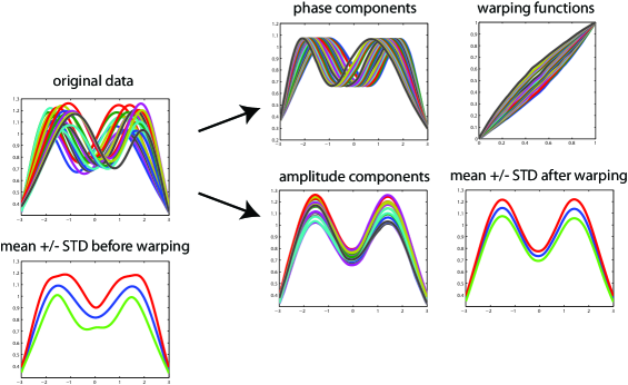
Figure 1: Separation of phase and amplitude variability in function data.

As another, more practical, example we consider the height evolution of subjects in the famous Berkeley growth data. Fig. 8 shows the time derivatives of the growth curves, for female and male subjects, to highlight periods of faster growth. Although the growth rates associated with different individuals are different, it is of great interest to discover broad common patterns underlying the growth data, particularly after aligning functions using time warping. Thus, one would like an automated technique for alignment of functions. Section 5 shows examples of data sets from the other applications studied in this paper, including handwriting curves, gene expression signals, and neuroscience spike trains.

In some applications it may be relatively easy to decide how to warp functions for a proper alignments. For instance, there may be some temporal landmarks that have to be aligned across observations. In that case the warping functions can be piecewise smooth (e.g. linear) functions that ensure that the landmarks are strictly aligned. This situation requires a manual specification of landmarks which can be a cumbersome process, especially for large datasets. In some other cases there may be some natural models that can be adopted for the warping functions. However, in general, one does not have such landmarks or natural warping functions, and needs a comprehensive framework where the alignment of observed functions is performed automatically in an unsupervised fashion. We seek a principled framework that will automatically estimate domain warpings of the observed functions in order to optimally align them. The two main goals of this paper are:

1. Joint Alignment and Comparison (Section 3): There are two distinct steps in the analysis of elastic functions: (1) warpings or registration of functions and (2) their comparison. An important requirement in our framework is that these two processes, warping and comparison, are performed in a single, unified framework, i.e. under a single objective function, as for example was done in [11]. A fundamental idea is to avoid treating warping as a pre-processing step where the individual functions are warped according to an objective function that is different from the metric used to compare them.

2. Signal Estimation Under Random Scales, Translations, and Warpings (Section 4): An application of this framework is in estimation of a signal under the following observation model. Let $f_{i}$ be an observation of a function $g$ under random scaling, random vertical translation, and random warping, and we seek an estimator for $g$ using $\{f_{i},i=1,2,\dots,n\}$. We will use this estimator for performing the alignment mentioned in the previous item.

Before we introduce our framework that achieves these goals, we present a brief summary of some past methods, and their strengths and limitations.

1.1 Past Techniques

There exists a large literature on statistical analysis of functions, in part due to the pioneering efforts of Ramsay and Silverman [16], Kneip and Gasser [10], and several others [14, 22]. When restricting to the analysis of elastic functions, the literature is relatively recent and limited [15, 5, 14, 22, 11]. There are basically two categories of the past papers on this subject. One set treats the problem of functional alignment or registration as a pre-processing step. Once the functions are aligned, they are analyzed using the standard tools from functional analysis, e.g the cross-sectional mean and covariance computation and PCA. The second set of papers study both comparison and analysis jointly, using energy-minimization procedures. Although the latter generally provides better results due to a joint solution, the choice of the energy function deserves careful scrutiny.

As an example for the first set, in [14], the authors use warping functions that are convex combinations of functions of the type: $\gamma_{i}(t)=\left({\int_{0}^{t}|f_{i}^{(\nu)}(s)|^{p}ds\over\int_{0}^{1}|f_{i}^{(\nu)}(s)|^{p}ds}\right)^{1/p}$, where $\nu$ and $p$ are two parameters, with the recommended values being $\nu=0$ and $p=1$. Then, the warped functions $\{f_{i}\circ\gamma_{i}\}$ are analyzed using standard statistical techniques under the Hilbert structure of square-intergable functions. Similarly, James [6] uses moment-based matching for aligning functions, followed up by the standard FPCA. The main problem with this approach is that the objective function for alignment is unrelated to the metric for comparing aligned functions. The two steps are conceptually disjoint and a change in the objective function for alignment may change the subsequent results.

We introduce some additional notation. Let $\Gamma$ be the set of orientation-preserving diffeomorphisms of the unit interval $[0,1]$: $\Gamma=\{\gamma:[0,1]\to[0,1]|\gamma(0)=0,\ \gamma(1)=1,\ \ \gamma\ \ \mbox{is a diffeo}\}$. Elements of $\Gamma$ form a group, i.e. (1) for any $\gamma_{1},\gamma_{2}\in\Gamma$, their composition $\gamma_{1}\circ\gamma_{2}\in\Gamma$; and (2) for any $\gamma\in\Gamma$, its inverse $\gamma^{-1}\in\Gamma$, where the identity is the self-mapping $\gamma_{id}(t)=t$. The role of $\Gamma$ in elastic function analysis is paramount. Why? For a function $f\in{\cal F}$, where ${\cal F}$ is an appropriate space of functions on $[0,1]$ (defined later), the composition $f\circ\gamma$ denotes the re-parameterization or a domain warping of $f$ using $\gamma$. Therefore, $\Gamma$ is also referred to as the re-parameterization or the warping group. In this paper we will use $\|f\|$ to denote $(\int_{0}^{1}|f(t)|^{2}dt)^{1/2}$, i.e., the standard $\mathbb{L}^{2}$ norm on the space of real-valued functions on $[0,1]$. A majority of past methods study the problem of registration and comparisons of functions, either separately or jointly, by solving:

$$\inf_{\gamma\in\Gamma}\|f_{1}-(f_{2}\circ\gamma)\|\$$ (1)

The use of this quantity is problematic because it is not symmetric. The optimal alignment of $f_{1}$ to $f_{2}$ gives a different minimum, in general, when compared to the optimal alignment of $f_{2}$ to $f_{1}$. One can enforce a symmetry in Eqn. 1 using a double optimization, i.e. by seeking a solution to the problem $\inf_{(\gamma_{1},\gamma_{2})\in\Gamma\times\Gamma}\|(f_{1}\circ\gamma_{1})-(f_{2}\circ\gamma_{2})\|$. However, this is a degenerate problem. Another way of ensuring symmetry is to solve: $\inf_{\gamma\in\Gamma}\|f_{1}-(f_{2}\circ\gamma)\|+\inf_{\gamma\in\Gamma}\|f_{2}-(f_{1}\circ\gamma)\|$. While this is symmetric, it still does not lead to a proper distance on the space of functions.

The basic quantity in Eqn. 1 is commonly used to form objective functions of the type:

$$E_{\lambda,i}[\nu]=\inf_{\gamma_{i}\in\Gamma}\left(\|(f_{i}\circ\gamma_{i})-\nu\|^{2}+\lambda\ \ {\cal R}(\gamma_{i})\right)\ ,\ \ i=1,2,\dots,n\ ,$$ (2)

where ${\cal R}$ is a smoothness penalty on the $\gamma_{i}$s to keep them close to $\gamma_{id}(t)=t$. The optimal $\gamma_{i}^{*}$ are then used to align the $f_{i}$s, followed by a cross-sectional analysis of the aligned functions. This procedure, once again, suffers from the problem of separation between the registration and the comparison steps. Another issue here is: What should $\nu$ be? It seems natural to use the cross-sectional mean of $f_{i}$s but that choice is problematic both empirically and conceptually (more on that later). Tang and Müller [22] use $\nu=f_{j}$, obtain a set of pairwise warping functions $\gamma_{ij}$ for each $i$, and average them to form the warping function for $f_{i}$. Kneip and Ramsay [11] take a template-based approach and use a different $\nu$ for each $i$, given by $\nu_{i}=\sum_{j=1}^{p}c^{i}_{j}\xi_{j}$. Here, the $\xi_{j}$s are certain basis elements that are also estimated from the data and, in turn, relate to the principal components of the observations. Although this formulation has the nice property of solving for the registration and the principal components simultaneously, it implicitly uses the quantity in Eqn. 1 to compute the residuals.

1.2 Proposed Approach

We are going to take a differential geometric approach that provides a natural and fundamental framework for alignment of elastic functions. This approach is motivated by recent developments in shape analysis of parametrized curves [27, 21]. The use of elastic functions for analysis of variance and clustering has also been studied in [9] and for analysis of spike train data in [26].

It is problematic to use the cross-sectional mean of $\{f_{i}\}$ in Eqn. 2 for finding optimal alignments. To understand this issue, consider the following estimation problem. Let $f_{i}=c_{i}(g\circ\gamma_{i})+e_{i}$, $i=1,2,\dots,n$, represent observations of a signal $g\in{\cal F}$ under random warpings $\gamma_{i}\in\Gamma$, scalings $c_{i}\in\mathbb{R}_{+}$ and vertical translations $e_{i}\in\mathbb{R}$, and we seek an estimator for $g$ given $\{f_{i}\}$. Note that estimation of $g$ is equivalent to the alignment of $f_{i}$s since, given $g$, one can estimate $\gamma_{i}$s and compute $f_{i}\circ\gamma_{i}^{-1}$ to align them. So, we focus on deriving an estimator for $g$. In this context, it is easy to see that the cross-sectional mean for $\{f_{i}\}$ is not an estimator of $g$. In fact, we claim that to derive an estimator for $g$ it is more natural to work in the quotient space ${\cal F}/\Gamma$ rather than ${\cal F}$ itself. This quotient space is the set of orbits of the types $[f]=\{(f\circ\gamma)|\gamma\in\Gamma\}$. We will show that the Karcher mean of the orbits $\{[f_{i}]\}$ is a consistent estimator of the orbit of $g$ and that a specific element of that mean orbit, selected using a pre-determined criterion, is a consistent estimator of $g$.

Now, the definition of Karcher mean requires a proper distance on ${\cal F}/\Gamma$. The quantity in Eqn. 1 cannot be used since $\|f_{1}-f_{2}\|\neq\|(f_{1}\circ\gamma)-(f_{2}\circ\gamma)\|$ for general $f_{1},f_{2}\in{\cal F}$ and $\gamma\in\Gamma$. (This point was also noted by Vantini [23] although the solution proposed [18], restricting to only the linear warpings, is not for general use.) Instead, we use $d_{FR}$, the distance resulting from the Fisher-Rao Riemannian metric, since the action of $\Gamma$ is by isometries under that metric. That is, $d_{FR}(f_{1},f_{2})=d_{FR}(f_{1}\circ\gamma,f_{2}\circ\gamma)$, for all $f_{1}$, $f_{2}$, and $\gamma$. Fisher-Rao Riemannian metric was introduced in 1945 by C. R. Rao [17] where he used the Fisher information matrix to compare different probability distributions. This metric was studied rigorously in the 70s and 80s by Amari [1], Efron [4], Kass [8], Cencov [3], and others. While those earlier efforts were focused on analyzing parametric families, we use the nonparametric version of the Fisher-Rao Riemannian metric in this paper. (This nonparametric form has found an important use in shape analysis of curves [21].) An important attribute of this metric is that it is preserved under warping, and Cencov [3] showed that it is the only metric with this attribute. It is difficult to compute the distance $d_{FR}$ directly under this metric but Bhattacharya [2] introduced a square-root representation that greatly simplifies this calculation. We will modify this square-root representations for use with more general functions.

2 Function Representation and Metric

In order to develop a natural and efficient framework for aligning elastic functions, we introduce a square-root representation of functions.

2.1 Representation Space of Functions

Let $f$ be a real-valued function on the interval $[0,1]$. We are going to restrict to those $f$ that are absolutely continuous on $[0,1]$; let ${\cal F}$ denote the set of all such functions. We define a mapping: $Q:\mathbb{R}\to\mathbb{R}$ according to: $Q(x)\equiv\left\{\begin{array}[]{cc}x/\sqrt{|x|}&\mbox{if}\ |x|\neq 0\\ 0&\ \ \mbox{otherwise}\end{array}\right.$. Note that $Q$ is a continuous map. For the purpose of studying the function $f$, we will represent it using a square-root velocity function (SRVF) defined as $q:[0,1]\to\mathbb{R}$, where $q(t)\equiv Q(\dot{f}(t))={\dot{f}(t)}/{\sqrt{|\dot{f}(t)|}}$. This representation includes those functions whose parameterization can become singular in the analysis. It can be shown that if the function $f$ is absolutely continuous, then the resulting SRVF is square integrable. Thus, we will define $\mathbb{L}^{2}([0,1],\mathbb{R})$ (or simply $\mathbb{L}^{2}$) to be the set of all SRVFs. For every $q\in\mathbb{L}^{2}$ there exists a function $f$ (unique up to a constant, or a vertical translation) such that the given $q$ is the SRVF of that $f$. In fact, this function can be obtained precisely using the equation: $f(t)=f(0)+\int_{0}^{t}q(s)|q(s)|ds$. Thus, the representation $f\Leftrightarrow(f(0),q)$ is invertible.

If we warp a function $f$ by $\gamma$, how does its SRVF change? The SRVF of $f\circ\gamma$ is given by: $\tilde{q}(t)={{d\over dt}(f\circ\gamma)(t)\over\sqrt{|{d\over dt}(f\circ\gamma)(t)|}}=(q\circ\gamma)(t)\sqrt{\dot{\gamma}(t)}$. We will denote this transformation by $(q,\gamma)=(q\circ\gamma)\sqrt{\dot{\gamma}}$. The motivations for using SRVF for functional analysis are many and to understand these merits we first present the relevant metric.

2.2 Elastic Riemannian Metric

In this paper we will use the Fisher-Rao Riemannian metric for analyzing functions. We remind the reader that a Riemmanian metric is a smoothly-varying inner product defined on the tangent spaces of the manifold.

Definition 1

For any $f\in{\cal F}$ and $v_{1},v_{2}\in T_{f}({\cal F})$, where $T_{f}({\cal F})$ is the tangent space to ${\cal F}$ at $f$, the Fisher-Rao Riemannian metric is defined as the inner product:

$$\left\langle\left\langle v_{1},v_{2}\right\rangle\right\rangle_{f}={1\over 4}\int_{0}^{1}\dot{v}_{1}(t)\dot{v_{2}}(t){1\over|\dot{f}(t)|}dt\ .$$ (3)

In case we are dealing only with functions such that $\dot{f}(t)\geq 0$, e.g. cumulative distribution functions or growth curves, then we obtain a more classical version of the Fisher-Rao metric. Thus, the above definition is a more general form of the Fisher-Rao metric, the one that deals with signed functions instead of just density functions.

This metric has many fundamental advantages, including the fact that it is the only Riemannian metric that is invariant to the domain warping [3], and has played an important role in information geometry. This metric is somewhat complicated since it changes from point to point on ${\cal F}$, and it is not straightforward to derive equations for computing geodesics in ${\cal F}$. For instance, the geodesic distance between any two points $f_{1},f_{2}\in{\cal F}$ is based on finding a geodesic path between them under the F-R metric. This minimization is non-trivial and only some numerical algorithms are known to attempt this problem. Once we find a geodesic path connecting $f_{1}$ and $f_{2}$ in ${\cal F}$, its length becomes the geodesic distance $d_{FR}$. However, a small transformation provide an enormous simplification of this task. This motivates the use of SRVFs for representing and aligning elastic functions.

Lemma 1

Under the SRVF representation, the Fisher-Rao Riemannian metric becomes the standard $\mathbb{L}^{2}$ metric.

Proof is given in the appendix. This result can be used to compute the distance $d_{FR}$ between any two functions as follows. Simply compute the $\mathbb{L}^{2}$ distance between the corresponding SRVFs and set $d_{FR}$ to that value: $d_{FR}(f_{1},f_{2})=\|q_{1}-q_{2}\|$. The next question is: What is the effect of warping on $d_{FR}$? This is answered by the following result.

Lemma 2

For any two SRVFs $q_{1},q_{2}\in\mathbb{L}^{2}$ and $\gamma\in\Gamma$, $\|(q_{1},\gamma)-(q_{2},\gamma)\|=\|q_{1}-q_{2}\|$.

See the appendix for the proof. In the case of functions with the non-negativity constraint (that is, $\dot{f}\geq 0$), this transformation was used by Bhattacharya [2].

2.3 Elastic Distance on Quotient Space

So far we have defined the Fisher-Rao distance on ${\cal F}$ and have found a simple way to compute it using SRVFs. But we have not involved any warping function in the distance calculation and thus it represents a non-elastic comparison of functions. The next step is to define an elastic distance between functions as follows. The orbit of an SRVF $q\in\mathbb{L}^{2}$ is given by: $[q]=\mbox{closure}\{(q,\gamma)|\gamma\in\Gamma\}\ =\mbox{closure}\{(q\circ\gamma)\sqrt{\dot{\gamma}})|\gamma\in\Gamma\}$. It is the set of SRVFs associated with all the warpings of a function, and their limit points. Any two elements of $[q]$ represent functions which have the same $y$ variability but different $x$ variability. Let ${\cal S}$ denote the set of all such orbits. To compare any two orbits we need a metric on ${\cal S}$. We will use the Fisher-Rao distance to induce a distance between orbits, and we can do that only because under this the action of $\Gamma$ is by isometries.

Definition 2

For any two functions $f_{1},\ f_{2}\in{\cal F}$ and the corresponding SRVFs, $q_{1},q_{2}\in\mathbb{L}^{2}$, we define the elastic distance $d$ on the quotient space ${\cal S}$ to be: $d([q_{1}],[q_{2}])=\inf_{\gamma\in\Gamma}\|q_{1}-(q_{2},\gamma)\|$.

Note that the distance $d$ between a function and its domain-warped version is zero. However, it can be shown that if two SRVFs belong to different orbits, then the distance between them is non-zero. Thus, this distance $d$ is a proper distance (i.e. it satisfies non-negativity, symmetry, and the triangle inequality) on ${\cal S}$ but not on $\mathbb{L}^{2}$ itself, where it is only a pseudo-distance.

Table 1 provides a quick summary of relationships between the Fisher-Rao metric and ${\cal F}$ on one hand, and the $\mathbb{L}^{2}$ metric and the space of SRVFs on the other.

Table 1. Bijective Relationship Between Function Space ${\cal F}$ and SRVF space $\mathbb{L}^{2}$

Item	Function Space ${\cal F}$	SRVF Space $\mathbb{L}^{2}$
Representation	$f$	$(q,f(0))$
Transformation	$f(t)=f(0)+\int_{0}^{t}q(s)|q(s)|ds$	$q(t)={\dot{f}(t)}/{\sqrt{|\dot{f}(t)|}}$
Metric	Fisher-Rao Metric	$\mathbb{L}^{2}$ Metric
	$\left\langle\left\langle v_{1},v_{2}\right\rangle\right\rangle_{\cal F}=\int_{0}^{1}\dot{v}_{1}(t)\dot{v}_{2}(t){1\over|\dot{f}(t)|}dt$	$\left\langle w_{1},w_{2}\right\rangle=\int_{0}^{1}w_{1}(t)w_{2}(t)dt$
Distance	$d_{FR}(f_{1},f_{2})$	$\|q_{1}-q_{2}\|$
Isometry	$d_{FR}(f_{1},f_{2})=d_{FR}(f_{1}\circ\gamma,f_{2}\circ\gamma)$	$\|q_{1}-q_{2}\|=\|(q_{1},\gamma)-(q_{2},\gamma)\|$
Geodesic	Numerical Solution	Straight Line
Elastic Distance	$d=\inf_{\gamma\in\Gamma}d_{FR}(f_{1},f_{2}\circ\gamma)$	$d=\inf_{\gamma\in\Gamma}\left(\|q_{1}-(q_{2}\circ\gamma)\sqrt{\dot{\gamma}})\|\right)$ in ${\cal S}$
between $f_{1}$ and $f_{2}$		Solved Using Dynamic Programming

3 Karcher Mean and Function Alignment

An important goal of this warping framework is to align the functions so as to improve the matching of features (peaks and valleys) across functions. A natural idea is to compute a cross-sectional mean of the given functions and then align the given functions to this mean template. The problem is that we do not have a proper distance function on $\mathbb{L}^{2}$, invariant to time warpings, that can be used to define a mean. But we have a distance function on the quotient space ${\cal S}$, so we will use a mean on that space to derive a template for function alignment. We will do so in two steps: First, for a given collection of functions $f_{1},f_{2},\dots,f_{n}$, and their SRVFs $q_{1},q_{2},\dots,q_{n}$, we compute the mean of the corresponding orbits $[q_{1}],[q_{2}],\dots,[q_{n}]$ in the quotient space ${\cal S}$; we will call it $[\mu]_{n}$. Next, we compute an appropriate element of this mean orbit to define a template $\mu_{n}$ in $\mathbb{L}^{2}$. Then, the alignment of individual functions comes from warping their SRVFs to match the template ${\mu}_{n}$ under the elastic distance.

We remind the reader that if $dist$ denotes the geodesic distance between points on a Riemannian manifold $M$, and $\{p_{i},i=1,2,\dots,n\}$ is a collection of points on $M$, then a local minimizer of the cost function $p\mapsto\sum_{i=1}^{n}dist(p,p_{i})^{2}$ is defined as the Karcher mean of those points [7]. It is also known by other names such as the intrinsic mean or the Fréchet mean. The algorithm for computing a Karcher mean is based on gradients and has become a standard procedure in statistics on nonlinear manifolds (see, for example [12]). We will not present the general procedure but will describe its use in our problem.

3.1 Karcher Mean of Points in $\Gamma$

In this section we will define a Karcher mean of a set of warping functions $\{\gamma_{i}\}$, under the Fisher-Rao metric, using the differential geometry of $\Gamma$. Analysis on $\Gamma$ is not straightforward because it is a nonlinear manifold. To understand its geometry, we will represent an element $\gamma\in\Gamma$ by the square-root of its derivative $\psi=\sqrt{\dot{\gamma}}$. Note that this is the same as the SRVF defined earlier for elements of ${\cal F}$, except that $\dot{\gamma}>0$ here. The identity element $\gamma_{id}$ maps to a constant function with value $\psi_{id}(t)=1$. Since $\gamma(0)=0$, the mapping from $\gamma$ to $\psi$ is a bijection and one can reconstruct $\gamma$ from $\psi$ using $\gamma(t)=\int_{0}^{t}\psi(s)^{2}ds$. An important advantage of this transformation is that since $\|\psi\|^{2}=\int_{0}^{1}\psi(t)^{2}dt=\int_{0}^{1}\dot{\gamma}(t)dt=\gamma(1)-\gamma(0)=1$, the set of all such $\psi$s is $\mathbb{S}_{\infty}$, the unit sphere in the Hilbert space $\mathbb{L}^{2}$. In other words, the square-root representation simplifies the complicated geometry of $\Gamma$ to the unit sphere. Recall that the distance between any two points on the unit sphere, under the Euclidean metric, is simply the length of the shortest arc of a great circle connecting them on the sphere. Using Lemma 1, the Fisher-Rao distance between any two warping functions is found to be $d_{FR}(\gamma_{1},\gamma_{2})=\cos^{-1}(\int_{0}^{1}\sqrt{\dot{\gamma}_{1}(t)}\sqrt{\dot{\gamma}_{2}(t)}dt)$. Now that we have a proper distance on $\Gamma$, we can define a Karcher mean as follows.

Definition 3

For a given set of warping functions $\gamma_{1},\gamma_{2},\dots,\gamma_{n}\in\Gamma$, define their Karcher mean to be $\bar{\gamma}_{n}=\mathop{\rm argmin}_{\gamma\in\Gamma}\sum_{i=1}^{n}d_{FR}(\gamma,\gamma_{i})^{2}$.

The search for this minimum is performed using Algorithm 1 as follows:
Algorithm 1: Karcher Mean of $\{\gamma_{i}\}$ Under $d_{FR}$:
Let $\psi_{i}=\sqrt{\dot{\gamma}_{i}}$ be the SRVFs for the given warping functions. Initialize $\mu_{\psi}$ to be one of the $\psi_{i}$s or use $w/\|w\|$, where $w={1\over n}\sum_{i=1}^{n}\psi_{i}$.

1. For $i=1,2,\dots,n$, compute the shooting vector $v_{i}={\theta_{i}\over\sin(\theta_{i})}(\psi_{i}-\cos(\theta_{i})\mu_{\psi})$, where $\theta_{i}=\cos^{-1}(\int_{0}^{1}\mu_{\psi}(t)\psi_{i}(t)dt)$.

2. Compute the average $\bar{v}={1\over n}\sum_{i=1}^{n}v_{i}$.

3. If $\|\bar{v}\|$ is small, then stop. Else, update $\mu_{\psi}\mapsto\cos(\epsilon\|\bar{v}\|)\mu_{\psi}+\sin(\epsilon\|\bar{v}\|){\bar{v}\over\|\bar{v}\|}$, for a small step size $\epsilon>0$ and return to Step 1.

4. Compute the mean warping function using $\bar{\gamma}_{n}=\int_{0}^{t}\mu_{\psi}(s)^{2}ds$.

3.2 Karcher Mean of Points in ${\cal S}=\mathbb{L}^{2}/\Gamma$

Next we consider the problem of finding means of points in the quotient space ${\cal S}$. Since we already have a well-defined distance on ${\cal S}$ (given in Definition 2), the definition of the Karcher mean follows.

Definition 4

Define the Karcher mean $[\mu]_{n}$ of the given SRVF orbits $\{[q_{i}]\}$ in the space ${\cal S}$ as a local minimum of the sum of squares of elastic distances:

$$[\mu]_{n}=\mathop{\rm argmin}_{[q]\in{\cal S}}\sum_{i=1}^{n}d([q],[q_{i}])^{2}\ .$$ (4)

We emphasize that the Karcher mean $[\mu]_{n}$ is actually an orbit of functions, rather than a function. That is, if $\mu_{0}$ is a minimizer of the cost function in Eqn. 4, then so is $(\mu_{0},\gamma)$ for any $\gamma$. The full algorithm for computing the Karcher mean in ${\cal S}$ is given next.

Algorithm 2: Karcher Mean of $\{[q_{i}]\}$ in ${\cal S}$

1. Initialization Step: Select $\mu=q_{j}$, where $j$ is any index in $\mathop{\rm argmin}_{1\leq i\leq n}||q_{i}-\frac{1}{n}\sum_{k=1}^{n}q_{k}||$.

2. For each $q_{i}$ find $\gamma_{i}^{*}$ by solving: $\gamma_{i}^{*}=\mathop{\rm argmin}_{\gamma\in\Gamma}\|\mu-(q_{i}\circ\gamma)\sqrt{\dot{\gamma}}\|$. The solution to this optimization comes from a dynamic programming algorithm. In cases where a solution does not exist in $\Gamma$, the dynamic programming algorithm still provides an approximation in $\Gamma$.

3. Compute the aligned SRVFs using $\tilde{q}_{i}\mapsto(q_{i}\circ\gamma_{i}^{*})\sqrt{\dot{\gamma_{i}^{*}}}$.

4. If the increment $\|{1\over n}\sum_{i=1}^{n}\tilde{q}_{i}-\mu\|$ is small, then stop. Else, update the mean using $\mu\mapsto{1\over n}\sum_{i=1}^{n}\tilde{q}_{i}$ and return to step 2.

The iterative update in Steps 2-4 is based on the gradient of the cost function given in Eqn. 4. Although we prove its convergence next, its convergence to a global minimum is not guaranteed. Denote the estimated mean in the $k$th iteration by $\mu^{(k)}$. In the $k$th iteration, let $\gamma_{i}^{(k)}$ denote the optimal domain warping from $q_{i}$ to $\mu^{(k)}$ and let $\tilde{q}_{i}^{(k)}=(q_{i}\circ\gamma_{i}^{(k)})\sqrt{\dot{\gamma}_{i}^{(k)}}$. Then, $\sum_{i=1}^{n}d([\mu^{(k)}],[q_{i}])^{2}=\sum_{i=1}^{n}\|\mu^{(k)}-\tilde{q}_{i}^{(k)}\|^{2}\geq\sum_{i=1}^{n}\|\mu^{(k+1)}-\tilde{q}_{i}^{(k)}\|^{2}\geq\sum_{i=1}^{n}d([\mu^{(k+1)}],[q_{i}])^{2}$. Thus, the cost function decreases iteratively and as zero is a natural lower bound, $\sum_{i=1}^{n}d([\mu^{(k)}],[q_{i}])^{2}$ will always converge.

3.3 Center of an Orbit

The remaining task is to find a particular element of this mean orbit so that it can be used as a template to align the given functions. Towards this purpose, we will define the center of an orbit using a condition similar to past papers, see e.g. [22], which says that the mean of the warping functions should be the identity. A major difference here is that we use the Karcher mean and not the cross-sectional mean as was done in the past.

Definition 5

For a given set of SRVFs $q_{1},q_{2},\dots,q_{n}$ and $q$, define an element $\tilde{q}$ of $[q]$ as the center of $[q]$ with respect to the set $\{q_{i}\}$ if the warping functions $\{\gamma_{i}\}$, where $\gamma_{i}=\mathop{\rm argmin}_{\gamma\in\Gamma}\|\tilde{q}-(q_{i},\gamma)\|$, have the Karcher mean $\gamma_{id}$.

We will prove the existence of such an element by construction.

Algorithm 3: Finding Center of an Orbit : WLOG, let $q$ be any element of the orbit $[q]$.

1. For each $q_{i}$ find $\gamma_{i}$ by solving: $\gamma_{i}=\mathop{\rm argmin}_{\gamma\in\Gamma}\left(\|q-(q_{i}\circ\gamma)\sqrt{\dot{\gamma}}\|\right)$.

2. Compute the mean $\bar{\gamma}_{n}$ of all $\{\gamma_{i}\}$ using Algorithm 1. The center of $[q]$ wrt $\{q_{i}\}$ is given by $\tilde{q}=(q,\bar{\gamma}_{n}^{-1})$.

This algorithm is depicted pictorially in Fig. 2

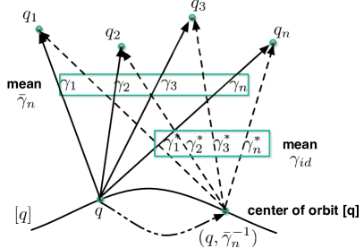
Figure 2: Finding center of the orbit $[q]$ with respect to the set $\{q_{i}\}$.

We need to show that $\tilde{q}$ resulting from Algorithm 3 satisfies the mean condition in Definition 5. Note that $\gamma_{i}$ is chosen to minimize $\|q-(q_{i},\gamma)\|$, and also that $\|\tilde{q}-(q_{i},\gamma)\|=\|(q,\bar{\gamma}_{n}^{-1})-(q_{i},\gamma)\|=\|q-(q_{i},\gamma\circ\bar{\gamma}_{n})\|$. Therefore, $\gamma_{i}^{*}=\gamma_{i}\circ\bar{\gamma}_{n}^{-1}$ minimizes $\|\tilde{q}-(q_{i},\gamma)\|$. That is, $\gamma_{i}^{*}$ is a warping that aligns $q_{i}$ to $\tilde{q}$. To verify the Karcher mean of $\gamma_{i}^{*}$, we compute the sum of squared distances $\sum_{i=1}^{n}d_{FR}(\gamma,\gamma_{i}^{*})^{2}=\sum_{i=1}^{n}d_{FR}(\gamma,\gamma_{i}\circ\bar{\gamma}_{n}^{-1})^{2}=\sum_{i=1}^{n}d_{FR}(\gamma\circ\bar{\gamma}_{n},\gamma_{i})^{2}$. As $\bar{\gamma}_{n}$ is already the mean of $\gamma_{i}$, this sum of squares is minimized when $\gamma=\gamma_{id}$. That is, the mean of $\gamma_{i}^{*}$ is $\gamma_{id}$.

We will apply this setup in our problem by finding the center of $[\mu]_{n}$ with respect to the given SRVFs $\{q_{i}\}$.

3.4 Complete Alignment Algorithm

Now we can utilize the three algorithms, Algorithm 1-3, to present the full procedure for finding a template $\mu_{n}$ that is used to align the individual functions.

Complete Alignment Algorithm: Given a set of functions $f_{1},f_{2},\dots f_{n}$ on $[0,1]$, let $q_{1},q_{2},\dots,q_{n}$ denote their SRVFs, respectively.

1. Computer the Karcher mean of $[q_{1}],\ [q_{2}],\dots,[q_{n}]$ in ${\cal S}$ using Algorithm 2. Denote it by $[\mu]_{n}$.

2. Find the center of $[\mu]_{n}$ wrt $\{q_{i}\}$ using Algorithm 3; call it $\mu_{n}$. (Note that this algorithm requires a step for computing the Karcher mean of warping functions using Algorithm 1).

3. For $i=1,2,\dots,n$, find $\gamma_{i}^{*}$ by solving: $\gamma_{i}^{*}=\mathop{\rm argmin}_{\gamma\in\Gamma}\|\mu_{n}-(q_{i},\gamma)\|$.

4. Compute the aligned SRVFs $\tilde{q}_{i}=(q_{i},\gamma_{i}^{*})$ and aligned functions $\tilde{f}_{i}=f_{i}\circ\gamma_{i}^{*}.$

5. Return the template $\mu_{n}$, the warping functions $\{\gamma_{i}^{*}\}$, and the aligned functions $\{\tilde{f}_{i}\}$.

3.5 Simulation Results

To illustrate this method we use a number of simulated datasets. Although our framework is developed for functions on $[0,1]$, it can easily be adapted to an arbitrary interval using a linear transformation.

1. Simulated Data 1: As the first example, we study a set of simulated functions used previously in [11]. The individual functions are given by: $y_{i}(t)=z_{i,1}e^{-(t-1.5)^{2}/2}+z_{i,2}e^{-(t+1.5)^{2}/2}$, $i=1,2,\dots,21$, where $z_{i,1}$ and $z_{i,2}$ are i.i.d normal with mean one and standard deviation $0.25$. Each of these functions is then warped according to: $\gamma_{i}(t)=6({e^{a_{i}(t+3)/6}-1\over e^{a_{i}}-1})-3$ if $a_{i}\neq 0$, otherwise $\gamma_{i}=\gamma_{id}$, where $a_{i}$ are equally spaced between $-1$ and $1$, and the observed functions are computed using $f_{i}(t)=y_{i}(\gamma_{i}(t))$. A set of 21 such functions forms the original data and is shown in the left panel of Fig. 3, and the remaining panels show the results of our method. The second panel presents the resulting aligned functions $\{\tilde{f}_{i}\}$ and the third panel plots the corresponding warping functions $\{\gamma_{i}^{*}\}$. The remaining panels show the cross-sectional mean and mean $\pm$ standard deviations of $\{f_{i}\}$ and $\{\tilde{f}_{i}\}$, respectively.

   $\{f_{i}\}$	$\{\tilde{f}_{i}\}$	$\{\gamma_{i}^{*}\}$	mean $\pm$ std, before	mean $\pm$ std, after

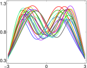
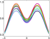
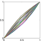
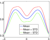
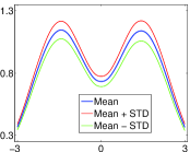
   Figure 3: Results on simulated data set 1.

   The plot of $\{\tilde{f}_{i}\}$ shows a tighter alignment of functions with sharper peaks and valleys. The two peaks are at $-1.5$ and $1.5$ which is exactly what we expect. This means that the effects of warping generated by the $\gamma_{i}$s have been completely removed and only the randomness from the $y_{i}$s remains. Also, the plot of mean $\pm$ standard deviation shows a thinning of bands around the mean due to the alignment.

2. Simulated Data 2: As a simple test of our method we analyze a set of functions with no underlying phase variability. To do this, we take $\{y_{i}\}$, as above, but this time we do not warp them at all; these functions are shown in the left panel of Figure 4. Note that, by construction, the two peaks in these functions are always aligned, only their amplitudes are different. There is a slight misalignment in the valleys between the two peaks due to differing mixture weights. The result of the alignment process is shown in the remaining panels. The second panel shows that the aligned functions are very similar to the original data, except for a better alignment of the valleys. The next panel shows the estimated warping functions which are very close to the identity. The last panel shows the means of the original and the aligned functions and they are practically identical.

   $\{f_{i}\}$	$\{\tilde{f}_{i}\}$	$\{\gamma_{i}^{*}\}$	mean, before and after

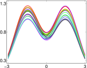
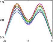
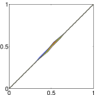
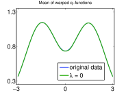
   Figure 4: Results on simulated data 2.

3. Simulated Data 3: In this case we take a family of Gaussian kernel functions with the same shape but with significant phase variability, in the form of horizontal shifts, and minor amplitude variation. Figure 5 shows the original $29$ functions $\{f_{i}\}$, the aligned functions $\{\tilde{f}_{i}\}$, the warping functions $\{\gamma_{i}^{*}\}$, and the before-and-after cross sectional mean and standard deviations. Once again we notice a tighter alignment of functions with only minor variability left in $\{\tilde{f}_{i}\}$ reflecting the differing heights in the original data. The remaining two plots show that mean $\pm$ standard deviation of the aligned data is far more compact than the raw data.

   $\{f_{i}\}$	$\{\tilde{f}_{i}\}$	$\{\gamma_{i}^{*}\}$	mean $\pm$ std, before	mean $\pm$ std, after

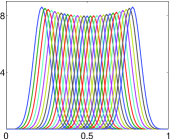
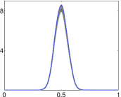
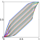
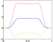
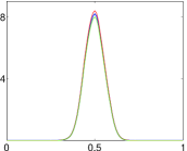
   Figure 5: Results on simulated data 3.

4. Simulated Data 4: In this case we take a family of multimodal wave functions with the same shape but different phase variations. The individual functions are defined on $[0,9]$ and given by: $f_{i}(t)=(1-(\gamma_{i}(t)/9-0.5)^{2})\sin(\pi\gamma_{i}(t))$, $i=1,2,\dots,9$, with the warping functions $\gamma_{i}(t)=9({e^{a_{i}t/9}-1\over e^{a_{i}}-1})$ if $a_{i}\neq 0$, otherwise $\gamma_{i}=\gamma_{id}$. Here $a_{i}$ are equally spaced between $-1.5$ and $1.5$ with step size $0.375$. Figure 6 shows the original $9$ functions $\{f_{i}\}$, the aligned functions $\{\tilde{f}_{i}\}$ (clearly showing the common shape), the warping functions $\{\gamma_{i}^{*}\}$, and the before-and-after cross sectional mean and standard deviations, again showing the huge difference in apparent amplitude variation between aligned and unaligned functions. In particular, with only the phase variability in the data, our method has a perfect alignment of given functions.

   $\{f_{i}\}$	$\{\tilde{f}_{i}\}$	$\{\gamma_{i}^{*}\}$	mean $\pm$ std, before	mean $\pm$ std, after

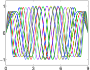
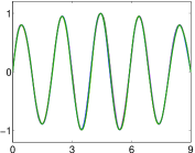
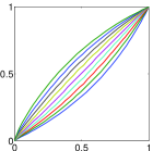
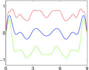
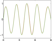
   Figure 6: Results on simulated data 4.

4 Signal Estimation and Estimator Consistency

In this section we justify the proposed framework by posing and solving a model-based estimation of alignment. Consider an observation model $f_{i}=c_{i}(g\circ\gamma_{i})+e_{i}$, $i=1,\dots,n,$ where $g$ is an unknown signal, and $c_{i}\in\mathbb{R}_{+}$, $\gamma_{i}\in\Gamma$ and $e_{i}\in{\cal F}$ are random. We will concentrate on a simpler problem where the observation noise $e_{i}$ is set to a constant and, given the observations $\{f_{i}\}$, the goal is to estimate the signal $g$ or, equivalently, the warping functions $\{\gamma_{i}\}$. This or related problems have been considered previously by several papers, including [25, 15], but we are not aware of any formal statistical solution. Here we show that the center $\mu_{n}$, resulting from the complete alignment algorithm, leads to a consistent estimator of $g$. The proofs of Lemmas and Corollary are given in the appendix.

Theorem 1

For a function $g$, consider a sequence of functions $f_{i}(t)=c_{i}g(\gamma_{i}(t))+e_{i}$, where $c_{i}$ is a positive constant, $e_{i}$ is a constant, and $\gamma_{i}$ is a time warping, $i=1,\cdots,n$. Denote by $q_{g}$ and $q_{i}$ the SRVFs of $g$ and $f_{i}$, respectively, and let $\bar{s}={1\over n}\sum_{i=1}^{n}\sqrt{c_{i}}$. Then, the Karcher mean of $\{[q_{i}],i=1,2,\dots,n\}$ in ${\cal S}$ is $\bar{s}[q_{g}]$. That is,

$$[\mu]_{n}\equiv\mathop{\rm argmin}_{[q]}\left(\sum_{i=1}^{N}d^{2}([q_{i}],[q])\right)=\bar{s}[q_{g}]=\bar{s}\{(q_{g},{\gamma}),{\gamma}\in\Gamma\}\ .$$

We will prove this theorem in two steps. First we establish the following useful result.

Lemma 3

For any $q_{1},q_{2}\in\mathbb{L}^{2}$ and a constant $c>0$, we have $\mathop{\rm argmin}_{\gamma\in\Gamma}\|q_{1}-(q_{2},\gamma)\|=\mathop{\rm argmin}_{\gamma\in\Gamma}\|cq_{1}-(q_{2},\gamma)\|$.

Corollary 1

For any function $q\in\mathbb{L}^{2}$ and constant $c>0$, we have $\gamma_{id}\in\mathop{\rm argmin}_{\gamma\in\Gamma}\|cq-(q,\gamma)\|$. Moreover, if the set $\{t\in[0,1]|q(t)=0\}$ has (Lebesgue) measure 0, $\gamma_{id}=\mathop{\rm argmin}_{\gamma\in\Gamma}\|cq-(q,\gamma)\|$.

Now we get back to the proof of Theorem 1. The SRVF of the function $f_{i}=c_{i}(g\circ\gamma_{i})+e_{i}$ is given by $q_{i}=\sqrt{c_{i}}(q_{g},\gamma_{i})$, $i=1,\cdots,n$. For any $q$, we get

$$d([q_{i}],[q]) = d([\sqrt{c_{i}}(q_{g},\gamma_{i})],[q])=\inf_{\gamma}\|\sqrt{c_{i}}(q_{g},\gamma_{i})-(q,\gamma)\|$$

$$= \inf_{\gamma}\|\sqrt{c_{i}}q_{g}-(q,\gamma\circ\gamma_{i}^{-1})\|=\inf_{\gamma}\|\sqrt{c_{i}}q_{g}-(q,\gamma)\|=d([\sqrt{c_{i}}q_{g}],[q]).$$

In the last line, the first equality is based on the isometry of the group action of $\Gamma$ on $\mathbb{L}^{2}$ and the second equality is based on the group structure of $\Gamma$.

For any given $q$, let $\gamma^{*}\in\mathop{\rm argmin}_{\gamma\in\Gamma}\|q_{g}-(q,\gamma)\|$. Then, using Lemma 3, $\gamma^{*}\in\mathop{\rm argmin}_{\gamma\in\Gamma}\|\sqrt{c_{i}}q_{g}-(q,\gamma)\|$. Therefore,

$$\sum_{i=1}^{n}d^{2}([q_{i}],[q])=\sum_{i=1}^{n}d^{2}([\sqrt{c_{i}}q_{g}],[q])=\sum_{i=1}^{n}\|\sqrt{c_{i}}q_{g}-(q,\gamma^{*})\|^{2}\geq\sum_{i=1}^{n}\|\sqrt{c_{i}}q_{g}-\bar{s}q_{g}\|^{2}\ .$$

The last inequality comes from the fact that $\bar{s}q_{g}$ is simply the mean of $\{\sqrt{c_{i}}q_{g}\}$ in $\mathbb{L}^{2}$ space. The equality holds if and only if $(q,\gamma^{*})=\bar{s}q_{g}$ or $q=(\bar{s}q_{g},{\gamma^{*}}^{-1})$.

Actually, for any element of $[\bar{s}q_{g}]$, say $(\bar{s}q_{g},\gamma)$ for any $\gamma\in\Gamma$, we have

$$\sum_{i=1}^{n}d^{2}([q_{i}],[(\bar{s}q_{g},\gamma)])=\sum_{i=1}^{n}d^{2}([\sqrt{c_{i}}q_{g}],[\bar{s}q_{g}])=\sum_{i=1}^{n}\|\sqrt{c_{i}}q_{g}-\bar{s}q_{g}\|^{2}\ .$$

Therefore, $\{(\bar{s}q_{g},\gamma)|\gamma\in\Gamma\}$ is the unique solution to the Karcher mean $[\mu]_{n}\equiv\mathop{\rm argmin}_{[q]}\sum_{i=1}^{n}d^{2}([q_{i}],[q]).\ \ \ \ \Box$

Next, we present a simple fact about the Karcher mean of warping functions, where the Karcher mean is given in Definition 3.

Lemma 4

Given a set $\{\gamma_{i}\in\Gamma|i=1,...,n\}$ and a $\gamma_{0}\in\Gamma$, if the Karcher mean of $\{\gamma_{i}\}$ is $\bar{\gamma}$, then the Karcher mean of $\{\gamma_{i}\circ\gamma_{0}\}$ is $\bar{\gamma}\circ\gamma_{0}$.

Theorem 1 ensures that $[\mu]_{n}$ belongs to the orbit of $[q_{g}]$ (up to a scale factor) but we are interested in estimating $g$ itself, rather than its orbit. Since we can write $g\circ\gamma_{i}$ as $(g\circ\gamma_{a})\circ(\gamma_{a}^{-1}\circ\gamma_{i})$, for any $\gamma_{a}\in\Gamma$, the function $g$ is not identifiable unless we impose an additional constraint on $\gamma_{i}$. The same goes for the random variables $c_{i}$ and $e_{i}$. Under the assumption that the population means of $\gamma_{i}^{-1}$, $c_{i}$, and $e_{i}$ are known, we will show in two steps that Algorithm 3, that finds the center of the orbit $[\mu]_{n}$, results in a consistent estimator for $g$.

Theorem 2

Under the same conditions as in Theorem 1, let $\mu=(\bar{s}q_{g},\gamma_{0})$, for $\gamma_{0}\in\Gamma$, denote an arbitrary element of the Karcher mean class $[\mu]_{n}=\bar{s}[q_{g}]$. Assume that the set $\{t\in[0,1]|\dot{g}(t)=0\}$ has Lebesgue measure zero. If the population Karcher mean of $\{\gamma_{i}^{-1}\}$ is $\gamma_{id}$, then the center of the orbit $[\mu]_{n}$, denoted by $\mu_{n}$, satisfies $\lim_{n\rightarrow\infty}{\mu}_{n}=E(\bar{s})q_{g}$.

Proof: In Algorithm 3, we first compute $\tilde{\gamma}_{i}=\mathop{\rm argmin}_{\gamma}\|(q_{i},\gamma)-\mu\|=\mathop{\rm argmin}_{\gamma}\|(\sqrt{c_{i}}(q_{g},\gamma_{i}),\gamma)-(\bar{s}q_{g},\gamma_{0})\|=\mathop{\rm argmin}_{\gamma}\|(\sqrt{c_{i}}q_{g},\gamma_{i}\circ\gamma\circ\gamma_{0}^{-1})-\bar{s}q_{g}\|$. Since the set $\{t\in[0,1]|\dot{g}(t)=0\}$ has measure zero, the set $\{t\in[0,1]|q_{g}(t)=0\}$ also has measure zero. Using Corollary 1, this above distance is uniquely minimized when $\gamma_{i}\circ\tilde{\gamma}_{i}\circ\gamma_{0}^{-1}=\gamma_{id}$, or $\tilde{\gamma}_{i}=\gamma_{i}^{-1}\circ\gamma_{0}$. Denote the Karcher mean of these warping functions $\{\tilde{\gamma}_{i}\}$ by $\bar{\gamma}_{n}$. Applying the inverse of this $\bar{\gamma}_{n}$ to $\mu$, we get $\mu_{n}=(\mu,\bar{\gamma}_{n}^{-1})$. As $n\rightarrow\infty$, the Karcher mean of $\tilde{\gamma}_{i}$ converges to its population mean which, by Lemma 4, is $\gamma_{0}$. Thus, $\mu_{n}\stackrel{{\scriptstyle n\rightarrow\infty}}{{\longrightarrow}}E(\bar{s})((q_{g},\gamma_{0}),\gamma_{0}^{-1})=E(\bar{s})q_{g}$.     $\Box$

This result shows that asymptotically one can recover the SRVF of the original signal using the Karcher mean of the SRVFs of the observed signals. Of course, one is really interested in the signal $g$ itself, rather than its SRVF. One can reconstruct $g$ using aligned functions $\{\tilde{f}_{i}\}$ generated by the Alignment Algorithm in Section 3. As discussed above, we further assume the population mean of $e_{i}$ is known.

Theorem 3

Under the same conditions as in Theorem 2, let $\gamma_{i}^{*}=\mathop{\rm argmin}_{\gamma}\|(q_{i},\gamma)-\mu_{n}\|$ and $\tilde{f}_{i}=f_{i}\circ\gamma_{i}^{*}$. If we denote $\bar{c}=\frac{1}{n}\sum_{i=1}^{n}c_{i}$ and $\bar{e}=\frac{1}{n}\sum_{i=1}^{n}e_{i}$, then $\lim_{n\rightarrow\infty}\frac{1}{n}\sum_{i=1}^{n}\tilde{f}_{i}=E(\bar{c})g+E(\bar{e})$.

Proof: In the proof for Theorem 2, $\tilde{\gamma}_{i}=\mathop{\rm argmin}_{\gamma}\|(q_{i},\gamma)-\mu\|=\mathop{\rm argmin}_{\gamma}\|(q_{i},\gamma)-(\mu_{n},\bar{\gamma}_{n})\|$. Hence $\gamma_{i}^{*}=\mathop{\rm argmin}_{\gamma}\|(q_{i},\gamma)-\mu_{n}\|=\tilde{\gamma}_{i}\circ\bar{\gamma}_{n}^{-1}=\gamma_{i}^{-1}\circ\gamma_{0}\circ\bar{\gamma}_{n}^{-1}$. This implies that $\tilde{f}_{i}=f_{i}\circ\gamma_{i}^{*}=(c_{i}(g\circ\gamma_{i})+e_{i})\circ(\gamma_{i}^{-1}\circ\gamma_{0}\circ\bar{\gamma}_{n}^{-1})=c_{i}(g\circ\gamma_{0}\circ\bar{\gamma}_{n}^{-1})+e_{i}$. As $\bar{\gamma}_{n}\rightarrow\gamma_{0}$ when $n\rightarrow\infty$, we have

$$\lim_{n\rightarrow\infty}\frac{1}{n}\sum_{i=1}^{n}\tilde{f}_{i}=E(\bar{c})(g\circ\gamma_{0})\circ\gamma_{0}^{-1}+E(\bar{e})=E(\bar{c})g+E(\bar{e}).$$

$g$	$\{f_{i}\}$	$\{\tilde{f}_{i}\}$	estimate of $g$	error w.r.t. $n$

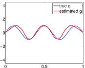
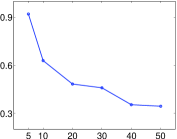
Figure 7: Example of consistent estimation.

Illustration. We illustrate the estimation process using an example with $g(t)=\sin(5\pi t)$, $t\in[0,1]$. We randomly generate $n=50$ warping functions $\{\gamma_{i}\}$ such that $\{\gamma_{i}^{-1}\}$ are i.i.d with mean $\gamma_{id}$. We also generate i.i.d sequences $\{c_{i}\}$ and $\{e_{i}\}$ from the exponential distribution with mean 1 and the standard normal distribution, respectively. Then we compute functions $f_{i}=c_{i}(g\circ r_{i})+e_{i}$ to form the functional data. In Fig. 7, the first panel shows the function $g$, and the second panel shows the data $\{f_{i}\}$. The Alignment Algorithm in Section 3 results in the aligned functions $\{\tilde{f}_{i}=f_{i}\circ\gamma_{i}^{*}\}$ that are are shown in the third panel in Fig. 7. Using Theorem 3, the original signal $g$ can be estimated by $(\frac{1}{n}\sum_{i=1}^{n}\tilde{f}_{i}-E(\bar{e}))/E(\bar{c})$. In this case, $E(\bar{c}))=1,E(\bar{e})=0$. This estimated $g$ (red) as well as the true $g$ (blue) are shown in the fourth panel. Note that the estimate is reasonably successful despite large variability in the raw data. Finally, we examine the performance of the estimator with respect to the sample size, by performing this estimation for $n$ equal to $5,10,20,30$, and $40$. The estimation errors, computed using the $\mathbb{L}^{2}$ norm between estimated $g$’s and the true $g$, are shown in the last panel. As expected from the earlier theoretical development, this estimate converges to the true $g$ when the sample size $n$ grows large.

5 Experimental Evaluation of Function Alignment

In this section we take functional data from several application domains and analyze them using the framework developed in this paper. Specifically, we will focus on function alignment and comparison of alignment performance with some previous methods on several datasets.

5.1 Applications on real data

We start with demonstrations of the proposed framework on some well known functional data.

1. Berkeley Growth Data: As a first example, we consider the Berkeley growth dataset for 54 female and 39 male subjects. For better illustrations, we have used the first derivatives of the growth curves as the functions $\{f_{i}\}$ in our analysis. (In this case, since SRVF is based on the first derivative of $f$, we actually end up using the second derivatives of the growth functions.)

The results from our elastic function analysis on the female growth curves are shown in Fig. 8 (left side). The top-left panel shows the original data. It can be seen from this plot that while the growth spurts for different individuals occurs at slightly different times, there are some underlying patterns to be discovered. This can also be observed in the cross-sectional mean and mean $\pm$ standard deviation plot in the bottom-left panel. In the second panel of the top row we show the aligned functions $\tilde{f}_{i}(t)$. The panel below it, which shows the cross-sectional mean and mean $\pm$ standard deviation, exhibits a much tighter alignment of the functions and, in turn, an enhancement of peaks and valleys in the aligned mean. In fact, this mean function suggests the presence of two growth spurts, one between 3 and 4 years, and the other between 10 and 12 years, on average. Similar analysis is performed on the male growth curves and Fig. 8 (right) shows the results: the original data (consisting of 39 derivatives of the original growth functions), the aligned functions $\tilde{f}_{i}(t)$, and the corresponding cross-sectional means and means $\pm$ standard deviations. The cross-sectional mean functions also show a much tighter alignment of the functions and, in turn, an enhancement of peaks and valleys in the aligned mean. This mean function suggests the presence of several growth spurts, between: 3 and 5, 6 and 7, and 13 and 14 years, on average.

Female Data		Male Data
original data	aligned functions	original data	aligned functions
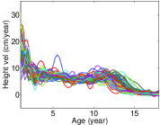
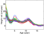
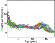
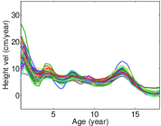
mean $\pm$ std, before	mean $\pm$ std, after	mean $\pm$ std, before	mean $\pm$ std, after

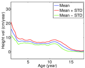
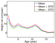
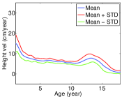
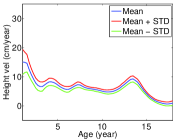
Figure 8: Analysis of growth data. Top: original data and the aligned functions. Bottom: the corresponding cross-sectional mean and mean $\pm$ standard deviations.

2. Handwriting Signature Data: As another example of the data that can be effectively modeled using elastic functions, we consider some handwritten signatures and the acceleration functions along the signature curves. This application was also considered in the paper [11]. Let $(x(t),y(t))$ denote the $x$ and $y$ coordinates of a signature traced as a function of time $t$. We study the acceleration functions $f(t)=\sqrt{\ddot{x}(t)^{2}+\ddot{y}(t)^{2}}$ for different instances of the signatures and study their variability after alignment.

The left panel in Fig. 9 shows the 20 acceleration functions of 20 signatures that are used in our analysis as $\{f_{i}\}$. The corresponding cross-sectional mean and mean $\pm$ standard deviations before the alignment are shown in the next panel. The right two panels show the aligned functions $\tilde{f}_{i}$s and the corresponding mean and mean $\pm$ standard deviations after the alignment. A look at the cross-sectional mean functions suggests that the aligned functions have much more exaggerated peaks and valleys, resulting from the alignment of these features due to warping.

original data	mean $\pm$ std, before	aligned functions	mean $\pm$ std, after

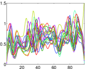
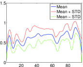
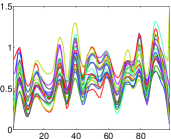
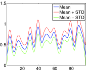
Figure 9: Analysis of signature profiles.

original data	mean $\pm$ std, before	aligned functions	mean $\pm$ std, after

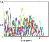
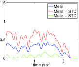
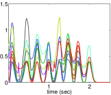
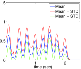
Figure 10: Analysis of spike train data.

3. Neuroscience Spike Data: Time-dependent information is represented via sequences of stereotyped spike waveforms in the nervous system. These waveform sequences (or spike trains) have been commonly looked as the language of the brain and are the focus of much investigation. Before we apply our framework, we need to convert the spike information into functional data. Assume $s(t)$ is a spike train with spike times $0<t_{1}<t_{2}<\cdots<t_{M}<T$, where $[0,1]$ denotes the recording time domain. That is, $s(t)=\sum_{i=1}^{M}\delta(t-t_{i}),\ \ t\in[0,1]\ ,$ where $\delta(\cdot)$ is the Dirac delta function. One typically smooths the spike trains to better capture the time correlation between spikes. In this paper we use a Gaussian kernel $K(t)=e^{-t^{2}/(2\sigma^{2})}/(\sqrt{2\pi}\sigma)$, $\sigma\geq 0$ ($\sigma=1ms$ here). That is, the smoothed spike train is $f(t)=(s*K)(t)=\sum_{i=1}^{M}\frac{1}{\sqrt{2\pi}\sigma}e^{-(t-t_{i})^{2}/(2\sigma^{2})}.$

Figure 10 left panel shows one example of such smoothed spike trains for 10 trials of one neurons in the primary motor cortex of a Macaque monkey subject that was performing a squared-path movement [26]. The next panel shows the cross-sectional mean and mean $\pm$ standard deviation of the functions in this neuron. The third panel shows $\{\tilde{f}_{i}\}$ where we see that the functions are well aligned with more exaggerated peaks and valleys. The next panel shows the mean and mean $\pm$ standard deviation. Similar to the growth data and signature data, an increased amplitude variation and decreased standard deviation are observed in this plot.

original data	mean $\pm$ std, before	aligned functions	mean $\pm$ std, after

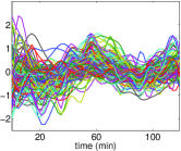
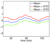
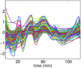
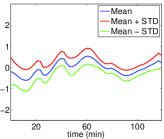
Figure 11: Analysis of gene expression data.

4. Gene Expression data: In this example, we consider temporal microarray gene expression profiles. The time ordering for yeast cell-cycle genes was investigated in [13], and we use the same data in this study. The expression level was measured during a period of 119 minutes for a total of 612 fully-recorded genes. There are 5 clusters with respect to phases in these continuous function. In particular, 159 of these functions were known to be related to M phase regulation of the yeast cell cycle. These 159 functions used here are same as those used in [13], and are shown in the left panel in Fig. 11. Although, in general, gene expression analysis has many goals and problems, we use focus only on the subproblem of expression alignment as functional data. The corresponding cross-sectional mean and mean $\pm$ standard deviations before the alignment are shown in the next panel. The right two panels show the aligned functions $\tilde{f}_{i}$s and the corresponding mean and mean $\pm$ standard deviations after the alignment. Once again we find a strong alignment of functional data with improved peaks and valleys.

5.2 Comparisons with other Methods

In this section we compare the results from our method to some of the past ideas where the software is available publicly. While we have compared our framework with other published work in conceptual terms earlier, in this section we focus on a purely empirical evaluation. In particular, we utilize several evaluation criteria for comparing the alignments of functional data in the several simulated and real datasets discussed in previous sections. The choice of an evaluation criteria is not obvious, as there is no single criterion that has been used consistently by past authors for measuring the quality of alignment. Thus, we use three criteria so that together they provide a more comprehensive evaluation. We will continue to use $f_{i}$ and $\tilde{f}_{i}$, $i=1,...,N$, to denote the original and the aligned functions, respectively.

1. Least Squares: A cross-validated measure of the level of synchronization [6]:

   $$ls=\frac{1}{N}\sum_{i=1}^{N}{\int(\tilde{f}_{i}(t)-\frac{1}{N-1}\sum_{j\neq i}{\tilde{f}_{j}}(t))^{2}dt\over\int({f}_{i}(t)-\frac{1}{N-1}\sum_{j\neq i}f_{j}(t))^{2}dt}\ ,$$ (5)

   $ls$ measures the total cross-sectional variance of the aligned functions, relative to the original value. The smaller the value of $ls$, the better the alignment is.

2. Pairwise Correlation: It measures pairwise correlation between functions:

   $$pc={\sum_{i\neq j}cc(\tilde{f}_{i}(t),\tilde{f}_{j}(t))\over\sum_{i\neq j}cc({f}_{i}(t),{f}_{j}(t))}\ ,$$ (6)

   where $cc(f,g)$ is the pairwise Pearson’s correlation between functions. The larger the value of $pc$, the better the alignment between functions in general.

3. Sobolev Least Squares: This time we compute the least squares using the first derivative of the functions:

   $$sls={\sum_{i=1}^{N}\int(\dot{\tilde{f}}_{i}(t)-\frac{1}{N}\sum_{j=1}^{N}\dot{\tilde{f_{j}}})^{2}dt\over\sum_{i=1}^{N}\int({\dot{f}}_{i}(t)-\frac{1}{N}\sum_{j=1}^{N}\dot{f_{j}})^{2}dt}\ ,$$ (7)

   This criterion measures the total cross-sectional variance of the derivatives of the aligned functions, relative to the original value, and is an alternative measure of the synchronization. The smaller the value of $sls$, the better synchronization the method achieves.

We compare our Fisher-Rao (F-R) method with the area under the curve (AUTC) method presented in [14], the Tang-Müller method [22] provided in principal analysis by conditional expectation (PACE) package, the self-modeling registration (SMR) method presented in [5], and the moment-based matching (MBM) technique presented in [6]. Fig. 12 summarizes the values of $(ls,pc,sls)$ for these five methods using 3 simulated and 4 real datasets. From the results, we can see that the F-R method does uniformly well in functional alignment under all the evaluation metrics. We have found that the $ls$ criterion is sometimes misleading in the sense that a low value can result even if the functions are not very well aligned. This is the case, for example, in the male growth data under SMR method. Here the $ls=0.45$, while for our method $ls=0.64$, even though it is easy to see that latter has performed a better alignment. On the other hand, the $sls$ criterion seems to best correlate with a visual evaluation of the alignment. Sometimes all three criteria fail to evaluate the alignment performance properly, especially when preserving the shapes of the original signals are considered. This is the case in the first row of the figure where the AUTC method has the same values of $ls$, $pc$, and $sls$ as our method but shapes of the individual functions have been significantly distorted. The wave function simulated data is the most challenging and no other method except ours does a good job. Another point of evaluation is the number of parameters used by different methods. While our method does not have any parameter to choose, the other methods involve choosing at least two but often more parameters which makes it challenging for a user to apply them in different scenarios.

Original	AUTC [14]	PACE [22]	SMR [5]	MBM [6]	F-R
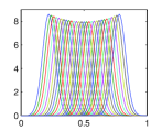
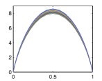
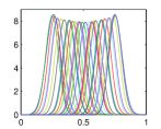
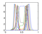
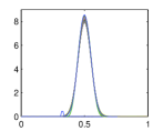
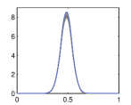
Gaussian kernel	(0.01, 11.0, 0.00)	(0.98, 1.18, 0.98)	(0.58, 2.86, 1.18)	(0.03, 10.3, 0.04)	(0.00, 11.0, 0.00)
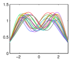
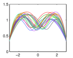
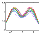
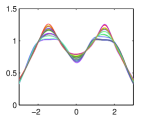
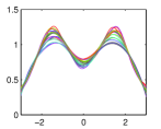
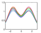
Bimodal	(0.89, 1.01, 0.82)	(0.49, 1.22, 0.23)	(0.11, 1.27, 0.30)	(0.16, 1.27, 0.29)	(0.29, 1.27, 0.04)
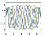
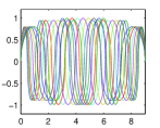
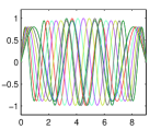
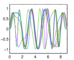
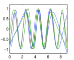
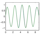
Wave function	(1.33, 2.12, 1.73)	(0.92, 13.0, 0.92)	(0.48, 83.7, 0.66)	(0.30, 124, 0.24)	(0.00, 175, 0.00)
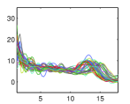
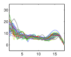
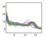
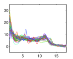
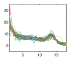
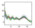
Growth-male	(1.10, 1.05, 0.55)	(0.91, 1.09, 0.68)	(0.45, 1.17, 0.77)	(0.70, 1.17, 0.62)	(0.64, 1.18, 0.31)
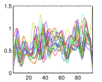
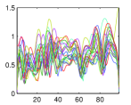
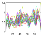
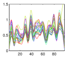
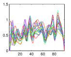
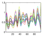
Signature	(1.00, 1.02, 0.99)	(0.91, 1.18, 0.84)	(0.62, 1.59, 0.31)	(0.64, 1.57, 0.46)	(0.56, 1.79, 0.31)
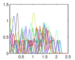
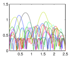
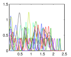
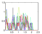
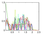
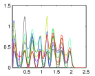
Neural data	(1.05, 0.27, 0.70)	(0.87, 1.35, 1.10)	(0.69, 2.54, 0.95)	(0.48, 3.06, 0.40)	(0.40, 3.77, 0.28)
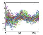
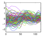
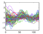
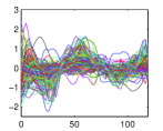
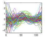
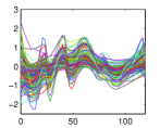
Gene expression data	(1.81, 0.65, 0.96)	(1.00, 1.14, 0.87)	(0.77, 1.53, 0.85)	(1.79, 0.72, 0.74)	(0.80, 2.36, 0.48)

Figure 12: Empirical evaluation of five methods on 3 simulated datasets and 4 real datasets, with the alignment performance computed using three criteria $(ls,pc,sls)$. The best cases are shown in boldface.

The computational costs associated with the different methods are given in Table 1. This table is for some of the datasets used in our experiments and are representative of the general complexities of these methods.

Method	AUTC [14]	PACE [22]	SMR [5]	MBM [6]	F-R
Software	Matlab	Matlab	Matlab	R	Matlab
Gaussian kernel	0.07sec	68sec	7.7sec	101sec	25sec
Bimodal	0.02sec	80sec	4.5sec	150sec	17sec
Growth-male	0.03sec	254sec	14.5sec	175sec	22sec
Signature	0.02sec	145sec	4.2sec	117sec	27sec

Table 1: Computational cost of the five methods some datasets used in Fig. 12.

6 Discussion

In this paper we have described a parameter-free approach for an automated alignment of given functions using time warping. The basic idea is to use the Fisher-Rao Riemannian metric and the resulting geodesic distance to define a proper distance, called elastic distance, between warping orbits of functions. This distance is used to compute a Karcher mean of the orbits, and a template is selected from the mean orbit using an additional condition that the mean of the warping functions is identity. Then, individual functions are aligned to the template using the elastic distance and a natural separation of the amplitude and phase variability of the function data is achieved. One interesting application of this framework is in estimating a signal observed under random time warpings. We propose the Karcher mean template as an estimator of the original signal and prove that it is a consistent estimator of the signal under some basic conditions on the random warping functions.

Important future directions in this work include: (1) the development of joint statistical models for the amplitude and phase components of the data, and (2) the use of such models for classification of observed functions into pre-determined classes. While the techniques for modeling the amplitude variability are quite common, e.g. using functional principal component analysis, the corresponding ideas for the phase component are relatively limited. The main reason is that $\Gamma$ is a nonlinear manifold and one cannot directly apply FPCA here. We mention that some solutions to this problem have been presented in [19, 20, 24] albeit in different contexts.

Appendix A Proofs of Lemmas 1 and 2

Proof of Lemma 1: The mapping from $f$ to $q$ is as follows: $f(t)\stackrel{{\scriptstyle{d\over dt}}}{{\rightarrow}}\dot{f}(t)\stackrel{{\scriptstyle Q}}{{\rightarrow}}q(t)$. For any $v\in T_{f}({\cal F})$, the differential of this mapping is: $v(t)\stackrel{{\scriptstyle{d\over dt}}}{{\rightarrow}}\dot{v}(t)\stackrel{{\scriptstyle Q_{*,f(t)}}}{{\rightarrow}}w(t)$. To evaluate the expression for $w$, we need the expression for $Q_{*}$. In case $x>0$, we have $Q(x)=\sqrt{x}$ and its directional derivative in the direction of $y\in\mathbb{R}$ is $y/(2\sqrt{x})$. In case $x<0$, we have $Q(x)=-\sqrt{-x}$ and its directional derivative in the direction of $y\in\mathbb{R}$ is $y/(2\sqrt{-x})$. Combining the two, the directional derivative of $Q$ is $Q_{*,x}(y)=y/(2\sqrt{|x|})$. Now, to apply this result to our situation, consider two tangent vectors $v_{1},v_{2}\in T_{f}({\cal F})$, and define their mappings under $Q_{*}$ as $w_{i}(t)\equiv Q_{*,\dot{f}(t)}(\dot{v}_{i}(t))=\dot{v}_{i}(t)/(2\sqrt{|\dot{f}(t)|})$. Taking the $\mathbb{L}^{2}$ inner-product between the resulting tangent vectors, we get: $\left\langle w_{1}(t),w_{2}(t)\right\rangle=\int_{0}^{1}w_{1}(t)w_{2}(t)dt={1\over 4}\int_{0}^{1}\dot{v}_{1}(t)\dot{v}_{2}(t){1\over|\dot{f}(t)|}dt$. The RHS is compared with Eqn. 3 to complete the proof. $\Box$

Proof of Lemma 2: For an arbitrary element $\gamma\in\Gamma$, and $q_{1},\ q_{2}\in\mathbb{L}^{2}$, we have: $\|(q_{1},\gamma)-(q_{2},\gamma)\|^{2}=\int_{0}^{1}(q_{1}(\gamma(t))\sqrt{\dot{\gamma}(t)}-q_{2}(\gamma(t))\sqrt{\dot{\gamma}(t)})^{2}dt=\int_{0}^{1}(q_{1}(\gamma(t))-q_{2}(\gamma(t)))^{2}\dot{\gamma}(t)dt=\|q_{1}-q_{2}\|^{2}\ .\Box$

Appendix B Proofs of Lemma 3, Corollary 1, and Lemma 4

Proof of Lemma 3: Using the definition: $\|cq_{1}-(q_{2},\gamma)\|^{2}=\int_{0}^{1}(cq_{1}(t)-(q_{2},\gamma)(t))^{2}dt=c^{2}\|q_{1}\|^{2}+\|q_{2}\|^{2}-2c\int_{0}^{1}q_{1}(t)(q_{2},\gamma)(t)dt$. Note that we have used $\|(q_{2},\gamma)\|^{2}=\|q_{2}\|^{2}$, an important fact, in the last equality. Thus,

$$\mathop{\rm argmin}_{\gamma\in\Gamma}\|q_{1}-(q_{2},\gamma)\|=\mathop{\rm argmax}_{\gamma\in\Gamma}\int_{0}^{1}q_{1}(t)(q_{2},\gamma)(t)dt=\mathop{\rm argmin}_{\gamma\in\Gamma}\|cq_{1}-(q_{2},\gamma)\|.\ \ \ \ \Box$$

Proof of Corollary 1: $\gamma_{id}\in\mathop{\rm argmin}_{\gamma\in\Gamma}\|cq-(q,\gamma)\|$ follows directly from Lemma 3 since $\gamma_{id}$ minimizes $\|q-(q,\gamma)\|$. Next we show that this minimizer is unique if the set $\{t\in[0,1]|q(t)=0\}$ has measure 0. In this case, if we define $F(t)=\int_{0}^{t}q(s)^{2}ds$, then $F$ is a strictly increasing function on $[0,1]$.

Using Lemma 3 again, we only need to show that $\gamma_{id}$ is the unique minimizer for $\|q-(q,\gamma)\|$. For any $\gamma^{*}\in\Gamma$ that minimizes $\|q-(q,\gamma)\|$, we have $\|q-(q,\gamma^{*})\|=\|q-(q,\gamma_{id})\|=0$. Therefore, $q(t)=q(\gamma^{*}(t))\sqrt{\dot{\gamma}^{*}(t)}$ (almost everywhere), and $F(t)=\int_{0}^{t}q(s)^{2}ds=\int_{0}^{t}q(\gamma^{*}(s))^{2}\dot{\gamma}^{*}(s)ds=\int_{0}^{\gamma^{*}(t)}q(r)^{2}dr=F(\gamma^{*}(t))$. As $F$ is strictly increasing, we must have $\gamma^{*}=\gamma_{id}$.    $\Box$

Proof of Lemma 4: First we observe that for any two $\gamma_{1},\gamma_{2}\in\Gamma$, we have $d_{FR}(\gamma_{1},\gamma_{2})=d_{FR}(\gamma_{1}\circ\gamma,\gamma_{2}\circ\gamma)$ for any $\gamma\in\Gamma$. This comes directly from the isometry of the group action of $\Gamma$ on itself (proof is similar to that of Lemma 2). This implies that: $\mathop{\rm argmin}_{\gamma}\sum_{i=1}^{n}d_{FR}(\gamma_{i}\circ\gamma_{0},\gamma)^{2}=\mathop{\rm argmin}_{\gamma}\sum_{i=1}^{n}d_{FR}(\gamma_{i},\gamma\circ\gamma_{0}^{-1})^{2}$. Let $\gamma^{*}$ denote the optimal $\gamma$ in the last term. Since $\mathop{\rm argmin}_{\gamma}\sum_{i=1}^{n}d_{FR}(\gamma_{i},\gamma)^{2}=\bar{\gamma}$, this implies that $\gamma^{*}\circ\gamma_{0}^{-1}=\bar{\gamma}$ or $\gamma^{*}=\bar{\gamma}\circ\gamma_{0}$.     $\Box$

References

- [1] S. Amari. Differential Geometric Methods in Statistics. Lecture Notes in Statistics, Vol. 28. Springer, 1985.
- [2] A. Bhattacharya. On a measure of divergence between two statistical populations defined by their probability distributions. Bull. Calcutta Math. Soc., 35:99–109, 1943.
- [3] N. N. Čencov. Statistical Decision Rules and Optimal Inferences, volume 53 of Translations of Mathematical Monographs. AMS, Providence, USA, 1982.
- [4] B. Efron. Defining the curvature of a statistical problem (with applications to second order efficiency). Ann. Statist., 3:1189–1242, 1975.
- [5] D. Gervini and T. Gasser. Self-modeling warping functions. Journal of the Royal Statistical Society, Ser. B, 66:959–971, 2004.
- [6] G. James. Curve alignments by moments. Annals of Applied Statistics, 1(2):480–501, 2007.
- [7] H. Karcher. Riemannian center of mass and mollifier smoothing. Comm. Pure and Applied Mathematics, 30(5):509–541, 1977.
- [8] R. E. Kass and P. W. Vos. Geometric Foundations of Asymptotic Inference. John Wiley & Sons, Inc., 1997.
- [9] D. Kaziska. Functional analysis of variance, discriminant analysis and clustering in a manifold of elastic curves. Communications in Statistics, 40:2487–2499, 2011.
- [10] A. Kneip and T. Gasser. Statistical tools to analyze data representing a sample of curves. The Annals of Statistics, 20:1266–1305, 1992.
- [11] A. Kneip and J. O. Ramsay. Combining registration and fitting for functional models. Journal of American Statistical Association, 103(483), 2008.
- [12] H. Le. Locating frechet means with application to shape spaces. Advances in Applied Probability, 33(2):324–338, 2001.
- [13] X. Leng and H. G. Müller. Time ordering of gene coexpression. Biostatistics, 7(4):569–584, 2006.
- [14] X. Liu and H. G. Müller. Functional convex averaging and synchronization for time-warped random curves. J. American Statistical Association, 99:687–699, 2004.
- [15] J. O. Ramsay and X. Li. Curve registration. Journal of the Royal Statistical Society, Ser. B, 60:351–363, 1998.
- [16] J. O. Ramsay and B. W. Silverman. Functional Data Analysis, Second Edition. Springer Series in Statistics, 2005.
- [17] C. R. Rao. Information and accuracy attainable in the estimation of statistical parameters. Bulletin of Calcutta Mathematical Society, 37:81–91, 1945.
- [18] L. M. Sangalli, P. Secchi, S. Vantini, and V. Vitelli. K-means alignment for curve clustering. Computational Statistics and Data Analysis, 54:1219–1233, 2010.
- [19] A. Srivastava, I. Jermyn, and S. H. Joshi. Riemannian analysis of probability density functions with applications in vision. IEEE Conference on Computer Vision and Pattern Recognition, 0:1–8, 2007.
- [20] A. Srivastava and I. H. Jermyn. Looking for shapes in two-dimensional, cluttered point clouds. IEEE Trans. on Pattern Analysis and Machine Intelligence, 31(9):1616–1629, 2009.
- [21] A. Srivastava, E. Klassen, S. H. Joshi, and I. H. Jermyn. Shape analysis of elastic curves in euclidean spaces. IEEE Transactions on Pattern Analysis and Machine Intelligence, in press, July 2011.
- [22] R. Tang and H. G. Müller. Pairwise curve synchronization for functional data. Biometrika, 95(4):875–889, 2008.
- [23] S. Vantini. On the definition of phase and amplitude variability in functional data analysis. MOX- Report No. 33, Dipartimento di Matematica, Politecnico di Milano, Via Bonardi 9 - 20133 Milano (Italy), 2009.
- [24] A. Veeraraghavan, A. Srivastava, A. K. Roy-Chowdhury, and R. Chellappa. Rate-invariant recognition of humans and their activities. IEEE Transactions on Image Processing, 8(6):1326–1339, June 2009.
- [25] K. Wang and T. Gasser. Alignment of curves by dynamic time warping. Annals of Statistics, 25(3):1251–1276, 1997.
- [26] W. Wu and A. Srivastava. Towards statistical summaries of spike train data. Journal of Neuroscience Methods, 195(1):107–110, 2011.
- [27] L. Younes. Computable elastic distance between shapes. SIAM Journal of Applied Mathematics, 58(2):565–586, 1998.