Geometric phases in a scattering process

Abstract

The study of geometric phase in quantum mechanics has so far be confined to discrete (or continuous) spectra and trace preserving evolutions. Consider only the transmission channel, a scattering process with internal degrees of freedom is neither a discrete spectrum problem nor a trace preserving process. We explore the geometric phase in a scattering process taking only the transmission process into account. We find that the geometric phase can be calculated by the some method as in an unitary evolution. The interference visibility depends on the transmission amplitude. The dependence of the geometric phase on the barrier strength and the spin-spin coupling constant is also presented and discussed.

Berry’s phase was originally introduced for bound states that an (discrete) eigenstate of the Hamiltonian would accumulate a geometric phaseberry84 , when the evolution of the system is adiabatic. This Berry’s phase provides us a very deep insight on the geometric structure of quantum mechanics and gives rise to various observable effects. The concept of the Berry phase has now become a central unifying concept in quantum mechanics, with applications in fields ranging from chemistry to condensed matter physics shapere89 . Recently the concept of Berry phase has been renewed and generalized for mixed stateserik00 ; tong04 ; yi04 . All these studies have been confined to discrete spectra.

For continuous spectrum, there are two things that can distinguish the geometric phase from bound states. (1) We always have non-Abelian gauge as a connection due to the degeneracy in this situation newton94 ; (2) The distortion of the Hamiltonian can not limited to a finite set of parameters, and hence we have to take into account the problem in an infinite-dimensional space. With these observations, the geometric phase factor has been considered for continuous spectra in newton94 , showing that the factor is exactly the scattering matrix. In Ref. ghosh96 , the scattering phase shift is defined in a way analogous to the adiabatic phase for bound states. This method works when reflection is negligible. By defining a virtual gap for the continuous spectrum through the notion of eigen-differential and using the differential projector operator, an explicit formula for a generalized geometrical phase is derived in terms of the eigenstates of the slowly time-dependent Hamiltonianmaamache08 . These studies, in contrast with the case of discrete spectra, are all for systems with continuous spectra.

A scattering process with particles that have (pseudo) spin degrees of freedom is a typical phenomenon different from the aforementioned: The (discrete) internal spin degrees of freedom of the scattering particles inevitably couple to the (continuous) motional dynamics tang95 . Hence such processes affect the state of the colliding spins according to quantum maps, instead of unitary operations. This makes the geometric phase acquired in such scattering processes distinct and interesting. Our main motivation in the present paper is to study the geometric phase in a scattering process with pseudo spin degrees of freedom. To tackle the problem, we focus on a gedanken setup consisting a quantum impurity, a mobile particle and two narrow potential barriers in each path of the double-slit, as shown in Fig. 1.

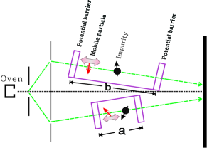
Figure 1: (Color online) Illustration of a gedanken setup. A mobile particle can propagate along a wire in each path. A quantum impurity and two narrow potential barriers lie at $-\frac{a}{2}$ and $\frac{a}{2}$ in one path, and at $-\frac{b}{2}$ and $\frac{b}{2}$ in another. Once the mobile particle injected into one of the path, it undergoes multiple reflections between the barriers and impurity. Eventually, the mobile particle transmitted froward or reflected back. Consider only the transmission channel, this scattering process is not of trace-preserving. $a$ ($b$) is the distance between the two barriers that we will refer to the width of structure in the text.

The mobile spin-1/2 particle $e$ can propagate along the 1D path. A quantum impurity $I$, modeled as a spin-$S$ scatterer, lies at $x=0$, whereas two narrow potential barriers are located at $x=\pm x_{0}$ (the $x$-axis is along the path, $x_{0}=a/2,b/2$ in Fig.1 for the two paths, respectively). The Hamiltonian for each path reads helman85 ; bose10 (we set $\hbar\!=\!1$ throughout)

$$H=\frac{p^{2}}{2m}+J\delta(x)\vec{s}\cdot\vec{S}+G\left[\delta(x-x_{0})+\delta(x+x_{0})\right],$$ (1)

where $m$ and $p$ are the effective mass and momentum operator of $e$, respectively, $\vec{s}$ and $\vec{S}$ stand respectively for the spin operators of $e$ and $I$, $J$ is a spin-spin coupling constant and $G$ is the potential-barrier strength. The above paradigmatic model naturally matches within a solid-state scenarios such as a 1D quantum wire davies98 or single-wall carbon nanotube devoret97 with an embedded magnetic impurity or quantum dotciccarello07 . Potential barriers are routinely implemented through applied gate voltages or heterojunctions.

Clearly, all of the scattering probability amplitudes are spin dependent due to the spin-spin contact potential $J\delta(x)\vec{s}\cdot\vec{S}$ in the Hamiltonian. As the overall spin space is $D$-dimensional ($D=[2\times(2S+1)]$), the effect of scattering is fully described by two $D\times D$ matrices whose generic elements respectively represent the amplitudes of reflection and transmission. These matrices can be derived by noting that the squared total spin of $e$ and $I$ as well as its projection along the $z$-axis are conserved. This entails that the dynamics within the singlet and triplet subspaces are decoupled. Consider only the transmission channel and assume that the injected state is

$$|\varphi_{in}\rangle=e^{ikx}|\uparrow\rangle\otimes|\phi_{m}\rangle,$$ (2)

the transmitted state takes,

$$|\varphi_{out}\rangle = e^{ikx}t_{\uparrow}|\uparrow\rangle\otimes|\phi_{m}\rangle+e^{ikx}t_{\downarrow}|\downarrow\rangle\otimes|\phi_{m+1}\rangle,$$ (3)

where $t_{\uparrow}$ and $t_{\downarrow}$ are the probability amplitudes for transmission with spin up and down, respectively. $|\phi_{m}\rangle$ are the eigenstates of $S_{z}$ (the $z$-component of $\vec{S}$), i.e., $S_{z}|\phi_{m}\rangle=m|\phi_{m}\rangle,$ and $k=\sqrt{2mE}$ with $E>0$ being the energy of the injected particle. $|\uparrow\rangle$ and $|\downarrow\rangle$ denote the eigenstates of $s_{z}$ for the mobile particle. The dependence of $t_{\uparrow}$ and $t_{\downarrow}$ on $G$, $J$ and $x_{0}$ can be established by

$$t_{\uparrow}=t_{\uparrow}(x_{0})=\{1+i[\chi-(m+1)j^{\prime}]\}/\Delta,$$ (4)

$$t_{\downarrow}=t_{\downarrow}(x_{0})=-ij^{\prime}F/\Delta,$$ (5)

where $j^{\prime}=|W|^{2}j/(2\kappa)$, $\Delta=(1+i\chi)[1+i(\chi-j^{\prime})]+S(S+1)j^{\prime 2}$ and $F=[(S-m)(S+m+1)]^{1/2}$, with $W=1+g\sin(2\kappa\alpha)+i2g\sin^{2}(\kappa\alpha),$ and $\chi=2g[g\sin(2\kappa\alpha)+\cos(2\kappa\alpha)].$ To simplify the problem, the following dimensionless quantities were defined: $j=J/(2a_{B}\epsilon)$, $\kappa=ka_{B}=\sqrt{E/\varepsilon}$, $g=G/(2ka_{B}\varepsilon)$, and $\alpha=x_{0}/a_{B}.$ Here $a_{B}$ is the Bohr radius, $\varepsilon=1/(2m)a_{B}^{2}$ and $2x_{0}$ is the distance between the two potential barriers, which we will call the width of structure in this paper.

Consider a situation where the width of the structure on each path is different but the spin-spin coupling constant and the barrier strength on both paths are the same. We have interests in the phase difference between the mobile particles transmitted through different paths. This phase difference consists of a dynamical phase and a geometrical part. Our task here is to extract the geometric phase from the total part $\Gamma=\arg\langle\varphi_{out}(a)|\varphi_{out}(b)\rangle.$ This can be done by either parallel transport of the state or canceling the dynamical phase. The parallel transport condition in this case is $\Im\langle\varphi_{out}(x_{0})|\frac{\partial}{\partial x_{0}}|\varphi_{out}(x_{0})\rangle=0$, leading to the geometric phase in the scattering process,

$$\gamma_{s}=\arg\left(\langle\varphi_{out}(a)|\varphi_{out}(b)\rangle e^{-i\Im(\int_{a}^{b}\frac{\langle\varphi_{out}(x_{0})|\frac{\partial}{\partial x_{0}}|\varphi_{out}(x_{0})\rangle}{\langle\varphi_{out}(x_{0})|\varphi_{out}(x_{0})}dx_{0})}\right),$$ (6)

where $\Im(...)$ denotes the imaginary part of $(...).$ We now prove that $\gamma_{s}$ defined in Eq. (6) is geometric, i.e., it only depends on the trajectory traced out by $|\varphi_{out}(x_{0})\rangle$. Define a quantum map by

$$M(b,a)=|\varphi_{out}(b)\rangle\langle\varphi_{out}(a)|,$$ (7)

the total phase $\Gamma$ acquired in the scattering process can be written as $\Gamma=\arg\langle\varphi_{out}(a)|M(b,a)|\varphi_{out}(a)\rangle.$ Notice that

$$\bar{M}(b,a)=M(b,a)e^{i\beta(b,a)}|\varphi_{out}(a)\rangle\langle\varphi_{out}(a)|$$ (8)

with real parameters $\beta(b,a)$ and $\beta(a,a)=0$ gives the same state $|\bar{\varphi}_{out}(b)\rangle$, since $|\bar{\varphi}_{out}(b)\rangle=e^{i\beta(b,a)}|\varphi_{out}(b)\rangle$ differs from $|\varphi_{out}(b)\rangle$ only in an overall phase $\beta(b,a)$. Parallel transport condition $\Im\langle\varphi_{out}(x_{0})|\frac{\partial}{\partial x_{0}}|\varphi_{out}(x_{0})\rangle=0$ leads to

$$\Im\langle\varphi_{out}(0)|\bar{M}^{\dagger}(x_{0},0)\frac{\partial}{\partial x_{0}}\bar{M}(x_{0},0)|\varphi_{out}(0)\rangle=0.$$ (9)

Substituting Eq. (8) into Eq.(9), we have

$$\beta(b,a)=-\int_{a}^{b}\frac{\Im\langle\varphi_{out}(x_{0})|\frac{\partial}{\partial x_{0}}|\varphi_{out}(x_{0})\rangle}{\langle\varphi_{out}(x_{0})|\varphi_{out}(x_{0})\rangle}dx_{0}.$$ (10)

This completes the proof. For our scattering problem, simple algebra yields,

$$\gamma_{s}=\arg\left[(t_{\uparrow}^{*}(a)t_{\uparrow}(b)+t_{\downarrow}^{*}(a)t_{\downarrow}(b))e^{-i\int_{a}^{b}\frac{1}{|t_{\uparrow}|^{2}+|t_{\downarrow}|^{2}}(|t_{\uparrow}|^{2}\frac{\partial\phi_{\uparrow}}{\partial x_{0}}+|t_{\downarrow}|^{2}\frac{\partial\phi_{\downarrow}}{\partial x_{0}})dx_{0}}\right].$$ (11)

Here, $\phi_{\uparrow(\downarrow)}$ was defined by

$$\tan\phi_{\uparrow(\downarrow)}\equiv\frac{t^{I}_{\uparrow(\downarrow)}}{t^{R}_{\uparrow(\downarrow)}}.$$

$t_{\uparrow(\downarrow)}^{I}$ and $t_{\uparrow(\downarrow)}^{R}$ denote the imaginary and real part of $t_{\uparrow(\downarrow)},$ respectively. The geometric phase given in Eq.(11) represents the difference in geometric phase for the mobile particle transmitted through the two paths. We will show later that it coincides with the geometric phase acquired in an unitary evolution treating the width as time $t$.

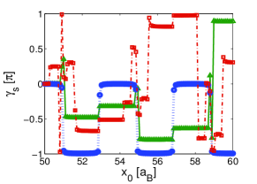
Figure 2: (Color online) The geometric phase $\gamma_{s}$ versus the width differences. Parameters chosen are: $J\rightarrow 0$ $(10^{-6})$ for blue circle; $J=11$ for red square and $J=50$ for green triangle. The other parameters: $k=0.8$, $a_{B}=1$, $G=10$, $m=-\frac{1}{2},$ $\varepsilon=1$, $S=\frac{1}{2}.$

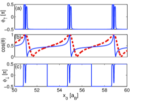
Figure 3: (Color online) Angle $\varphi_{\uparrow}$ and $\varphi_{\downarrow}$, and $\cos(\theta)$ as a function of the width differences. $J=50$ was taken for the plot. The red dashed line in (b) is for $J=11$. The other parameters chosen are the same as in Fig.2. $\cos\theta$ was defined by $\cos\theta\equiv\frac{|t_{\uparrow}|}{\sqrt{|t_{\uparrow}|^{2}+|t_{\downarrow}|^{2}}}$.

We have performed numerical calculations for Eq.(11), results are presented in Fig.2– Fig.5. For simplicity, $S=\frac{1}{2}$ was specified without loss of generality. Fig.2 shows the dependence of the geometric phase $\gamma_{s}$ on the width difference (i.e., $b-a$ in Fig.1) on the two paths for different spin-spin coupling constant. We find that the mobile particle acquires either $0$ or $-\pi$ geometric phase when $J\rightarrow 0$ ($J=10^{-6}$ was taken for the plot). Sharp changes in the geometric phase happen periodically, regardless of what value $J$ takes. Moreover we find that the geometric phase change its value only at the points where $t_{\uparrow}$ and $t_{\downarrow}$ change abruptly, as shown in Fig.3. We observe three resonances from Fig.3, corresponding to $\cos\theta=1.$ As the spin-spin coupling constant $J$ approaches the barrier strength $G$, the resonance region becomes wide (see the red-dashed line in Fig.3(b)).

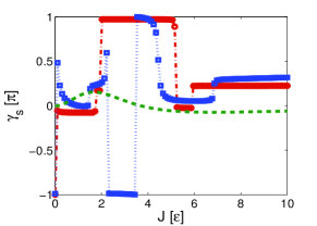
Figure 4: (Color online) $\gamma_{s}$ versus spin-spin coupling constant $J$. $G=0.1$ for green dashed line, $G=9$ for blue square line, and $G=30$ for red circle line. For other parameters, see Fig. 2. The width difference between the two pathes is $60a_{B}$.

Further examination shows that these points coincide with the condition for resonant energies given by $\cot(2\kappa\alpha)=-g$ (i.e., $|t_{\uparrow}|=1$). The spin-spin coupling smooth the sharpness of the changes, this is due to the broadening of the energy resonance (see Fig. 3, red dashed line). The dependence of the geometric phase on the spin-spin coupling is shown in Fig.4. Note that $\gamma_{s}=0$ when $G=0$, which is not shown on the figure. This can be easily interpreted in the limit of $g\rightarrow 0$. In this limit, $t_{\uparrow}\simeq(1-i0.5j^{\prime})/(1-ij^{\prime}+1.5j^{\prime 2}),$ $t_{\downarrow}\simeq(-ij^{\prime})/(1-ij^{\prime}+1.5j^{\prime 2}).$ Clearly, both $t_{\uparrow}$ and $t_{\downarrow}$ do not depend on the width of the structure, thus the system can not acquire a geometric phase with $G=0$. This is, however, not the case for $J=0$ as Fig.5 shows. In limit of $J=0$, $t_{\uparrow}\simeq\frac{1}{1+i\chi}$, and $t_{\downarrow}\simeq 0.$ As $\chi$ depends on the width, the geometric phase in this case is,

$$\gamma_{s}=\arg\left(t^{*}_{\uparrow}(a)t_{\uparrow}(b)e^{-i(\phi_{\uparrow}(a)-\phi_{\uparrow}(b))}\right).$$ (12)

In the strong spin-spin coupling ($J\rightarrow\infty$) and large barrier strength limit ($g\rightarrow\infty$), we have $\phi_{\uparrow}=\phi_{\downarrow}$ and $t_{\downarrow}=2t_{\uparrow},$ this leads to the geometric phase,

$$\gamma_{s}=\arg\left(t^{*}_{\uparrow}(a)t_{\uparrow}(b)e^{-i2(\phi_{\uparrow}(a)-\phi_{\uparrow}(b))}\right).$$ (13)

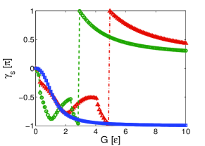
Figure 5: (Color online) $\gamma_{s}$ as a function of the barrier strength. $J\rightarrow 0$ for blue square line, $J=11$ for green circle, and $J=30$ for red triangle. The width difference between the two pathes is $60a_{B}$.

Now we are in a position to explore what is the difference between the normalized and non-normalized transmitted state, in terms of geometric phase. To this end, we define

$$\cos\theta\equiv\frac{|t_{\uparrow}|}{\sqrt{|t_{\uparrow}|^{2}+|t_{\downarrow}|^{2}}},$$

the transmitted state can be rewritten as,

$$|\varphi_{out}\rangle=\cos\theta e^{i\phi_{\uparrow}}|\uparrow\rangle\otimes|\phi_{m}\rangle+\sin\theta e^{i\phi_{\downarrow}}|\downarrow\rangle\otimes|\phi_{m+1}\rangle.$$ (14)

We point out that by the conservation of current probability, $|t_{\uparrow}|^{2}+|t_{\downarrow}|^{2}=1-|r_{\uparrow}|^{2}-|r_{\downarrow}|^{2}\leq 1.$ Here we consider only the transmission channel, and the transmitted state has been normalized, this would only affect the visibility of the interference fringes but not shift the patterns. By the definition of geometric phase for an unitary evolution, we have

$$\gamma^{\prime}_{s}=\arg\left((\cos\theta(b)\cos\theta(a)e^{i(\phi_{\uparrow}(b)-\phi_{\uparrow}(a))}+\sin\theta(b)\sin\theta(a)e^{i(\phi_{\downarrow}(b)-\phi_{\downarrow}(a))})e^{-i\int_{a}^{b}(\dot{\phi}_{\uparrow}\cos^{2}\theta+\dot{\phi}_{\downarrow}\sin^{2}\theta)dx_{0}}\right),$$ (15)

where $\dot{\phi}_{\uparrow}\equiv\frac{\partial\phi_{\uparrow}}{\partial x_{0}},~{}\dot{\phi}_{\downarrow}\equiv\frac{\partial\phi_{\downarrow}}{\partial x_{0}}.$ Recall that the real part of $\langle\varphi_{out}(a)|\varphi_{out}(b)\rangle$ represents the visibility of the interference pattern, we conclude that the geometric phase for the non-normalized and normalized transmitted state are the same, namely, $\gamma^{\prime}_{s}=\gamma_{s}$. One may concern about the observation of the geometric phase, inparticulare worry about the separation of the geometric phase from the total phase. In general, by varying the width difference $(b-a)$, it is possible to make the dynamics part of phase the same for the two beams.

In conclusion, the geometric phase in a scattering process is studied in this paper. Consider only the transmission channel, the scattering process is neither a trace-preserving dynamics nor a discrete spectrum problem. Instead it concerns the coupling between the internal degrees of freedom and the motional dynamics, and it can be described by quantum map to replace the unitary evolution. We have defined and calculated the geometric phase in such a process and show the dependence of the geometric phase on the spin-spin coupling constant and the barrier strengths. Possible observation of the geometric phase is suggested and discussed.    
This work is supported by NSF of China under grant Nos 61078011 and 10935010.

References

(1) M. V. Berry, Proc. R. Soc. London A 392, 45(1984).
(2) Geometric phase in physics, Edited by A. Shapere and F. Wilczek (
World Scientific, Singapore, 1989).
(3) E. Sjöqvist, A.K. Pati, A. Ekert, J.S. Anandan, M. Ericsson,
D.K.L. Oi, and V. Vedral, Phys. Rev. Lett. 85, 2845 (2000).
(4) D. M. Tong, E. Sjöqvist, L. C. Kwek, C. H. Oh, Phys. Rev. Lett.
93, 080405 (2004).
(5)X.X. Yi, L.C. Wang, and T.Y. Zheng, Phys. Rev. Lett. 92, 150406
(2004); X. X. Yi, and E. Sjöqvist, Phys. Rev. A 70, 042104 (2004);
L. C. Wang, H. T. Cui, and X. X. Yi, Phys. Rev. A 70, 052106 (2004).
(6) R. G. Newton, Phys. Rev. Lett 72, 954 (1994).
(7) G. Ghosh, Phys. Lett. A 210, 40 (1996).
(8) M. Maamache and Y. Saadi, Phys. Rev. Lett. 101, 150407 (2008).
(9) Z. Tang and D. Finkelstein, Phys. Rev. Lett. 74, 3134 (1995).
(10) O. L. T. de Menezes and J. S. Helman, Am. J.
Phys. 53, 1100 (1985).
(11) G. Cordourier-Maruri, F. Ciccarello, Y. Omar, M.
Zarcone, R. de Coss, and S. Bose, arXiv:1008.2370.
(12) J. H. Davies The Physics of Low-Dimensional Semiconductors: an Introduction
(Cambridge University Press, Cambridge, U.K., 1998)
(13) S. J. Tans, M. H. Devoret, H. Dai H, A. Thess, R. E. Smalley,
L. J. Geerligs , and C. Dekker, Nature 386, 474 (1997).
(14) F. Ciccarello et al., New J. Phys. 8, 214 (2006);
J. Phys. A: Math. Theor. 40, 7993 (2007);
F. Ciccarello, G. M. Palma, and M. Zarcone, Phys. Rev. B 75, 205415 (2007);
F. Ciccarello, M. Paternostro, G. M. Palma and M. Zarcone, Phys. Rev. B 80, 165313 (2009).