Refining Recency Search Results with User Click Feedback

Abstract

Traditional machine-learned ranking systems for web search are often trained to capture stationary relevance of documents to queries, which has limited ability to track non-stationary user intention in a timely manner. In recency search, for instance, the relevance of documents to a query on breaking news often changes significantly over time, requiring effective adaptation to user intention. In this paper, we focus on recency search and study a number of algorithms to improve ranking results by leveraging user click feedback. Our contributions are three-fold. First, we use real search sessions collected in a random exploration bucket for reliable offline evaluation of these algorithms, which provides an unbiased comparison across algorithms without online bucket tests. Second, we propose a re-ranking approach to improve search results for recency queries using user clicks. Third, our empirical comparison of a dozen algorithms on real-life search data suggests importance of a few algorithmic choices in these applications, including generalization across different query-document pairs, specialization to popular queries, and real-time adaptation of user clicks.

1 Introduction

Ranking a list of documents based on their relevance to a given query is the central problem in various search applications of the Internet. Machine-learned ranking algorithms have been shown highly effective for generalizing to unseen data from labeled training data and have been very successful especially in commercial Web search engines; see [18, 3, 4, 12, 6, 30, 23] and many references therein for more reference. Usually, such machine-learned ranking algorithms learn a ranking function based on editorial judgments—relevance labels provided by human editors. A critical assumption here is that the relevance of documents for a given query is more or less stationary over time, and therefore, as long as the coverage of training set is broad enough, the ranking function learned from the training set would be sufficient to generalize to unseen data in the future. This assumption is often valid in web search, especially for popular queries like “yahoo”, for which document relevance is indeed (almost) static.

However, there are other important categories of applications where document relevance to a query may change over time. One such example is the recency ranking problem in web search: when breaking news emerges, a document that used to be most relevant to a query may be superseded by others that have more relevant information about the news; see Section 3 for a concrete example. A key challenge for such problems is to track user intention in a timely fashion.

An interesting attempt was taken recently for tracking non-stationary document relevance [8]. The authors devised time-varying features that reflect freshness of documents and utilized recency demoted labels provided by human editors that explicitly modify the relevance target values in the training set. Their results showed an improvement of ranking qualities for time-sensitive queries. However, their approach is still based on editorial judgments and so limited for two reasons. First, obtaining high-quality training data is hard. Implementing more fine-grained time-varying features, such as features from the time series of clicks that can accurately follow the relevance drifts is considerably subtle and complex since carefully testing and selecting good features is a long and complicated process. Also, obtaining laborious recency demoted labels from human editors not only is expensive, but also can be inaccurate in correctly representing the temporal variation of document relevance. Second, even when we can come up with such complex and expensive data to batch-train a ranking function, tracking actual user intention remains challenging due to the very unpredictable nature of how user intention evolves over time.

In this paper, we investigate how to leverage user click feedback to complement and improve such editorial-judgment based ranking systems. Our rationale is that, particularly for recency queries, instantaneous click trends on the top portion of the ranking list are important indicators of document relevance. Such signals allow us to extract subtle information that may be hard for human editors to foresee when they provide relevance judgments. In particular, we explicitly track the click-through rate (CTR) of a query-document pair using a linear combination of extracted features, including the editorial-judgment based ranking function’s score. Based on search results returned by the current search engine, we propose a re-ranking approach to further improve search results for recency queries. We use user click as labels for training the CTR models in either batch or online mode.

In order to reliably evaluate and compare our algorithms, an “exploration bucket” was set up for a small random portion of live traffic for recency-classified queries in a commercial search engine. Within the bucket, the top URLs returned by the search engine was randomly shuffled. This bucket is critical to the work reported in this paper for two reasons. First, it provides a mechanism for exploration that is essential for interactive learning problems as the one considered in this paper to get rid of evaluation bias (Section 2). Second, it allows us to obtain unbiased evaluation of algorithms without the need for online bucket tests (Section 5.1).

This work extensively augments our preliminary results reported in an extended abstract [24], and uses random exploration data to do unbiased evaluation on a dozen of algorithms that improve ranking by leveraging user click feedback on a major web search engine.

The rest of the paper is organized as follows. We describe our exploration bucket in Section 2. Using data in this bucket, we present a motivating example in Section 3, showing the necessity of taking into account temporal variation of document relevance reflected in user click feedback. Our methods are detailed in Section 4 and empirically evaluated using the exploration bucket data in Section 5. We then discuss related work in Section 6 and conclude the paper in Section 7.

2 Exploration Bucket Data

As described in the previous section, we set up a bucket to collect exploration data from a small portion of live traffic from a commercial search engine. The bucket started on Jan 29, 2010 and ended on Feb 4, 2010. Throughout these days, we collected $399,880$ search sessions that contained 61,904 recency classified queries, after removing non-random sessions corrupted by business rules. The ranked list for those queries were generated by the recency ranking function trained as described in [8] and the ranking score for each query-document was recorded. For each session, we randomly shuffled the top four results and logged the permutation id of each shuffled permutation (a total of $4!=24$ of them) and user clicks on the corresponding permuted ranking results.

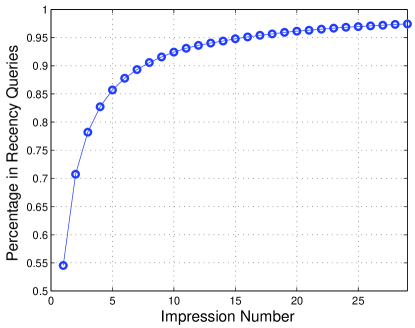
Figure 1: Recency query impression.

The collected data is very sparse and long-tailed as shown in Figure 1, in which $92.4\%$ of queries were issued no more than $10$ times and more than half of queries were issued just once. The reason for this sparsity is that the recency query classifier utilizes some language model to determine the queries that are related to each other, which causes some recency-related idiosyncratic, less popular queries—such as different word orderings or typographically wrong queries—to be classified as recency queries.

By doing the random shuffling, we are able to collect user click feedback on each document without positional bias, and such feedback can be thought of as a reliable proxy on relevance of documents. Note that the effect on user experience of shuffling would not be as severe as that for navigational queries, since the relevance differences of top-ranked documents to recency queries would not be as dramatic as those for navigational queries. Also, we chose a reasonably small number, $4$, in order to limit the negative impact on user experience in the exploration bucket.

Figure 2: Marginal nCTRs of four types of URL at the top four positions in exploration bucket, along with the nCTRs on the original order as control. All are on logarithm scale.

Another byproduct of our exploration bucket is that we can accurately observe the positional biases of clicks. Specifically, for the top four URLs in each session, we can infer the original ranking of the search engine simply by the recorded ranking scores. For each session, the URL with a highest ranking score is called the “1st URL”. These URLs were displayed an equal number of times in all four positions in the exploration bucket because of the random shuffling. We can then estimate the aggregate Click-through rate (CTR) of the 1st URLs in each of the four positions, as depicted by the blue line in Figure 2. Such nCTRs are marginal since we have taken all possible layouts (of other URLs) into account, thanks to the uniform randomness in the exploration bucket. Similarly, marginal nCTRs of the 2nd, 3rd, and 4th URLs of all sessions are also plotted in Figure 2.

Interestingly, lines of these four marginal nCTRs are almost parallel to each other, which implies the user click patterns follow the well-known power-law distribution. The slope indicates the intrinsic positional biases in the displayed layout of search results. To further illustrate the conditional effect on user click patterns, we also present the nCTRs of the original display order. It corresponds to the steeper straight line of Figure 2, indexed by “Control” in cyan. We observed that the nCTR of the 2nd URL at the 2nd position conditioned on the 1st URL at the 1st position is much lower than the marginal CTR of the 2nd URL at the 2nd position. The drop indicates a negative conditional effect from the 1st URL at the 1st position. For the 3rd URL at the 3rd position and the 4th URL at the 4th positions, we observed the similar conditional effect.

The apparent positional biases shown in Figure 2 would be taken into account below in devising our re-ranking algorithm. Moreover, the fact that the four lines other than the “Control” do not cross each other shows that, on average, the original ranking is doing a decent job in ranking the URLs also with respect to CTRs. However, in this paper, we show that we can do better than this by re-ranking the URLs appropriately so that the overall CTRs of re-ranked results can be further improved.

3 Motivation

Before running into technical details, let us first look at a concrete example found in exploration bucket to illustrate our motivation, and then summarize the challenges that we confront in recency search results. This example will be revisited in our discussion of experimental results.

As in [8, Section 4], recency queries are defined to be time-sensitive queries that show non-stationary temporal statistics compared to the past query logs. The query, “giant squid in California”, is a typical recency query, which appeared on February 1, 2010 and then disappeared after two days in our exploration bucket data. Figure 3 shows the impression statistics of the query with respect to time.

Figure 3: Impression count in the exploration bucket of the query “giant squid in California”.

This query is related to local news in California. At that time, a number of giant squids weighing up to 60 pounds had swum into waters off the Californian coast and were caught by sport fishermen by the hundreds. To find related materials of the local news, many people submitted the query “giant squid in California” to search engines.

Figure 4: Hourly CTR of the top 4 URLs associated with the recency query “giant squid in California”. After the 30th hour, no more click of this query was observed in the exploration bucket.

To study user click patterns on the URLs associated with the query, we again examined the top four URLs in the exploration bucket. The four URLs were retrieved by the default ranking function for recency queries in the search engine, which was trained on editorial judgments in batch mode. The ranking generated by the search engine on the four URLs was:

1. foxnews.com/story/0,2933,290667,00.html

2. en.wikipedia.org/wiki/Giant_Squid_(band)

3. metroactive.com/metro/03.29.06/squid-0613.html

4. youtube.com/watch?v=I3ENZDFkAow

Based on their contents, the four web pages can be categorized as “a news story page”, “a background knowledge page”, “a relevant page”, and “a video page”. As we randomly shuffled the display order of the top 4 URLs in the exploration bucket, each URL had the same chance to be displayed at each position. Therefore, position bias on clicks for these URLs was removed. The nCTRs of the four URLs observed in our exploration bucket session data are presented in Figure 4. Clearly, although the initial nCTRs were similar, the “video” content ended up receiving most clicks, while the “news story” was runner-up. This shows that while our recency ranking function made a reasonable decision (by putting the “video” content within top 4), it yet failed to accurately predict the ranking with respect to the users’ preference reflected in the CTR patterns on the URLs. Moreover, we note that unless we actually see this click patterns, it would be extremely hard for human editors to predict such relevance patterns.

Based on the above observations, two challenges are identified for the recency ranking problem.

• Relevance Drifting: As illustrated by the case above, document relevance may vary significantly over time. The above examples show the limitations of the editorial judgment based, batch learning framework in tracking such temporal dynamics. In general, it is very difficult to design features that can correctly reflect the temporal variances of relevance and for editors to predict the relevance labels before observing the actual user behaviors. How to rapidly track such drift would be a major challenge of recency ranking.

• Data Sparsity: Due to the reason specified in Section 2, many recency queries have few impressions. Hence, learning across queries (i.e., generalization) would be important.

In addition, we note that keeping track of dynamic content for recency queries to generate reasonably good top documents is also a critical challenge, but, it is outside the scope of the paper. In the present work, we rely on the baseline search engine to retrieve the most relevant documents, and focus on improved re-ranking using click feedback.

4 Our method

To address the two challenges in the previous subsection, we believe that it is helpful for a ranking module to detect and track the non-stationarity of user interests reflected on the click patterns. The example in Section 3 suggests that, when positional biases are removed, CTRs can be important indicators of relevances of URLs, especially for recency queries. Moreover, as shown in Figure 2, it is also important to remove positional biases and conditional effects in CTR estimates for documents. To this end, we assume that CTR at the top position, denoted by CTR@1, is of minimal conditional effect, and thus, we use CTR@1 as a proxy of relevance of a URL for learning and evaluating our method.

Ideally, if we knew the true CTR@1 of every document for a query, we could display the document with the highest CTR@1 at the top position. However, keeping track of CTR@1 of all query-document pairs is unnecessarily difficult: similar to general Web search, it is more important to get better estimates for high-quality documents for queries. Therefore, assuming that our original ranking function retrieves reasonably good quality documents at the top, we propose a re-ranking approach that estimates CTR@1 of top-ranked documents retrieved by the current search engines and then optimizes the ranking order by CTR@1 estimates. Our approach is designed specifically to address the challenges mentioned in Section 3 for recency queries:

• Relevance Drifting: In contrast to waiting for editorial judgments to update ranking results for a recency query, our algorithm updates CTR estimates near real-time based on user click feedback on the ranked list of documents. Not only does it avoid the expensive editorial judgments, but it can also quickly adapt to the varying relevance and then maximize CTR.

• Data Sparsity: Our algorithm works in a common feature space shared by all query–document pairs. It is then able to generalize click feedback of a pair to other pairs via feature values. Furthermore, we will also show the benefits of maintaining bias terms, or latent features, dedicated to popular query–document pairs in the experimental results.

One may question the appropriateness of using CTR@1 as a target for ranking problems. However, this choice is justified, particularly for the recency ranking problem, for the following reasons. First, CTR@1 is already an important metric that is considered for deploying general machine-learned ranking function for web search in practice. Second, our example in Section 3 shows that CTR@1 can be a more objective metric than editorial labels for the recency queries, for which relevance judgments are difficult to obtain. Third, our approach does not completely ignore editorial judgments, because only the top portion of ranking result list is refined. Since the baseline ranking list is obtained based on editorial labels, traditional relevance-oriented metrics like NDCG (Normalized Discounted Cumulative Gain) [16] are already reasonably high. Finally, it is worth noting that our approach can also be used to maximize other metrics of interest such as session length or revenue. With these reasonings, we now describe the setting and algorithm of our approach more in detail.

4.1 Settings

We consider the following re-ranking framework, naturally modeled as a round-by-round process: at round $t$,

1. A user arrives and types in a query $q_{t}$.

2. The default recency ranking function generates an ordered list of $s$ documents with highest relevance scores. Then, our re-ranking function re-orders these $s$ documents and present to the user the re-ordered ranked list $\{u_{t,1},\ldots,u_{t,s}\}$.

3. The user then provides feedback $r_{t}=\{c_{t,1},\ldots,c_{t,s}\}$ on our re-ranking result, where $c_{t,i}=1$ if a user clicked on the document at potision $i$, and $0$ otherwise.

4. Based on the user feedback $r_{t}$, the re-ranking function is updated and is used for the next round $t+1$.

From above described process, we see that our re-ranking function is inherently an online algorithm that updates its logic on the fly from the sequential observation of click feedback. In order to efficiently implement and update our re-ranking function, we implement a common feature vector for every query-document pair, $(q,u)$, and denote it as $\mathbf{x}_{qu}\in\mathbb{R}^{d}$. In our experiment, a total of $d=51$ features were used. These features include regular query-specific (e.g., number of words in a query), document-specific (e.g., spam classification score of a document), and query-document-specific (e.g., number of times a query appears in a given document) features used in ordinary machine learned ranking functions, and more importantly, the ranking score generated by the default, editorial judgment-based recency ranking function. Our re-ranking function is then defined to be a function that predicts the CTR@1 of each $(q,u)$ as a function of $\mathbf{x}_{qu}$ and possibly of some latent features, and the function gets updated based on observing users’ click feedback in an online fashion. The detailed function form and update formula are described in the subsequent two sections.

Given our goal of maximizing CTR@1 in the re-ranking results, it is tempting for an online algorithm to follow a greedy strategy: that is, it always ranks (for the present query at hand) the documents in the order of the highest CTR@1 estimates and updates the function parameters solely based on the user feedback for the algorithm’s ordered list. While this greedy approach is intuitively desirable, it can be detrimental in practice. This is because, as can be seen in the interactive round-by-round process described above, the re-ranking algorithm obtains user feedback only from the orderings that it has displayed to the user. Therefore, if an algorithm mistakenly orders the documents, a greedy re-ranking strategy can prevent it from collecting user feedback for other (potentially better) rankings and correcting its mistake to find the most relevant document on the top for maximizing CTR@1. Consequently, the algorithm has to balance two conflicting goals: (a) “exploitation” — to display in the first position most relevant documents to maximize re-ranking quality (in our case, to maximize user clicks), and (b) “exploration” — to display documents for the purpose of collecting data to further improvement. The exploration/exploitation tradeoff described above is a defining characteristic of a class of problems known as bandit problems [27], which has received considerable attention recently for Internet-related applications [25, 29].

In the following Section 4.2 and Section 4.3, we present the basic function form of our online re-ranking function and its update formula provided the user feedback $r_{t}$ is given, respectively. Then, in Section 4.4, we describe how we vary our scheme in order to cope with the explore/exploit tradeoff explained above and accelerate learning speed.

4.2 Parametric CTR@1 Estimate

Although many alternatives exist, we choose our re-ranking function to be linear in the feature vector $\mathbf{x}_{qu}$. This choice allows us to derive exact update rules and simplify the exposition. Other non-linear models may also be used, although numerical approximation is unavoidable in general when optimizing their model parameter. In particular, we have tried logistic regression and the probit-based regression [13], and observed similar performance as the linear model.

Since we try to maximize CTR@1, it is natural to find a function that estimates CTR@1 of a $(q,u)$ pair for re-ranking. Once the feature vector ${\mathbf{x}}_{qu}$ of length $d$ is given for a $(q,u)$ pair, a linear combination of them is used to estimate CTR@1. In fact, we will use the most general form that captures all variants useful in our experiments:

$$\text{CTR@1}(q,u) = \boldsymbol{\beta}^{{\top}}{\mathbf{x}}_{qu}+b_{q,u},$$ (1)

where the vector $\boldsymbol{\beta}\in\mathbb{R}^{d}$ contains the coefficients shared by all query-document pairs, and $b_{q,u}\in\mathbb{R}$ is a $(q,u)$-specific bias term. Both $\boldsymbol{\beta}$ and $\{b_{q,u}\}$ are to be learned by our algorithm.

Clearly, user click feedback on any query-document pair may be used to estimate $\boldsymbol{\beta}$, which in turn can be used to predict CTR@1 for other query-document pairs. Therefore, the linear part of $\boldsymbol{\beta}$ in Equation 1 addresses the data sparsity challenge by allowing generalization across different queries and documents. However, a linear model in the features may not be sufficiently accurate to capture the real CTR@1. The bias terms thus provide a mechanism to correct the residuals and to yield more accurate estimates. Due to these bias terms, it may appear that Equation 1 uses too many free parameters. However, as will be cleared in the next subsection, we use regularization to control the magnitude of these terms, so the bias terms will be essentially zero except for popular query-document pairs. Consequently, these terms can be used to yield a highly accurate CTR@1 estimate for popular $(q,u)$, while for unpopular $(q,u)$ (which suffer the data sparsity issue most) we essentially use the linear estimate $\boldsymbol{\beta}^{{\top}}{\mathbf{x}}_{qu}$. Such a dichotomy is done automatically within the regularization framework.

4.3 Parameter Update Rule

This subsection addresses the problem of parameter updates for model (1). We first describe how to fit the parameters if we are given a static set of data, then extend the update rule to the online case when data arrive sequentially, and finally discuss a few practical issues when deploying the update rules in large-scale ranking systems.

4.3.1 Batch Parameter Fitting

Suppose we are given a set $\mathcal{D}$ of $t$ data in the form of $\{(q_{i},u_{i},c_{i})\}_{i=1,2,\ldots,t}$, where $c_{i}\in\{0,1\}$ is the click feedback for $(q_{i},u_{i})$ provided by the $i$-th user. Let $\mathcal{P}$ be the set of distinct $(q,u)$ pairs observed in $\mathcal{D}$, and $N=|\mathcal{P}|$. For brevity, denote the feature vector for the $(q_{i},u_{i})$ pair as ${\mathbf{x}}_{i}$.

A standard approach to learn the parameters in Equation 1 for CTR@1 estimation is the ridge regression by using $\{c_{i}\}$’s as targets: we seek the optimal parameters that minimize a regularized square loss:

$$f_{t}(\boldsymbol{\beta},\{b_{q,u}\}) {\stackrel{{\scriptstyle\mathrm{def}}}{{=}}} \sum_{i=1}^{t}\left(c_{i}-\boldsymbol{\beta}^{\top}{\mathbf{x}}_{i}-b_{q_{i}u_{i}}\right)^{2}+\lambda_{1}\big{\|}\boldsymbol{\beta}-\boldsymbol{\beta}^{(0)}\big{\|}_{2}^{2}+\lambda_{2}\sum_{(q,u)\in\mathcal{P}}\big{\|}b_{qu}-b_{qu}^{(0)}\big{\|}_{2}^{2},$$ (2)

where $\lambda_{1}$ and $\lambda_{2}$ are positive regularization parameters provided by uers, $\boldsymbol{\beta}^{(0)}$ and $b_{qu}^{(0)}$ are the prior values, and $\|\cdot\|_{2}$ is the ordinary $\ell_{2}$-norm. Here, regularization is applied to avoid over-fitting and to ensure numerical stability.

Since (2) is a least-squares problem with $d+N$ many parameters, one may think it is intractable to solve for the exact solution since the computation complexity is $O((d+N)^{3})$ and $N$ is often very large. Fortunately, using matrix algebra, we can derive a closed-form solution for the minimizer of (2), whose complexity is cubic in $d$ and only linear in $N$.

Specifically, we partition the index set $\{1,2,\ldots,t\}$ into $I_{1}\cup I_{2}\cup\cdots\cup I_{N}$, so that $I_{j}$ contains indices in $\mathcal{D}$ that corresponds to the $j$-th distinct $(q,u)$ pair. For every $j\in\{1,2,\ldots,N\}$, we define the following quantities,

$$a_{j} {\stackrel{{\scriptstyle\mathrm{def}}}{{=}}} \lambda_{2}+|I_{j}|,$$

$${\mathbf{b}}_{j} {\stackrel{{\scriptstyle\mathrm{def}}}{{=}}} \sum_{i\in I_{j}}{\mathbf{x}}_{i},$$

$$d_{j} {\stackrel{{\scriptstyle\mathrm{def}}}{{=}}} \lambda_{2}b^{(0)}+\sum_{i\in I_{j}}c_{i}.$$

In addition, we define

$${\mathbf{A}}_{0} {\stackrel{{\scriptstyle\mathrm{def}}}{{=}}} \lambda_{1}{\mathbf{I}}+\sum_{i=1}^{t}{\mathbf{x}}_{i}{\mathbf{x}}_{i}^{\top},$$

$${\mathbf{d}}_{0} {\stackrel{{\scriptstyle\mathrm{def}}}{{=}}} \lambda_{1}\boldsymbol{\beta}^{(0)}+\sum_{i=1}^{t}c_{i}{\mathbf{x}}_{i}.$$

Now the optimal solution to the least-squares problem must satisfy the first-order optimality condition:

$$\frac{\partial f_{t}(\boldsymbol{\beta},\{b_{q,u}\})}{\partial\boldsymbol{\beta}} = \boldsymbol{0},$$

$$\frac{\partial f_{t}(\boldsymbol{\beta},\{b_{q,u}\})}{\partial b_{j}} = 0,$$

for each $j\in\{1,\ldots,N\}$. Solving this system of linear equations immediately gives the regularized least-squares solution:

$$\boldsymbol{\beta}^{*} = \left({\mathbf{A}}_{0}-\sum_{j=1}^{N}a_{j}^{-1}{\mathbf{b}}_{j}{\mathbf{b}}_{j}^{\top}\right)^{-1}\left({\mathbf{d}}_{0}-\sum_{j=1}^{N}a_{j}^{-1}d_{j}{\mathbf{b}}_{j}\right)$$ (3)

$$b_{j}^{*} = a_{j}^{-1}\left(d_{j}-{\mathbf{b}}_{j}^{\top}\boldsymbol{\beta}^{*}\right),\ \ \text{for each}\ \ j\in\{1,2,\ldots,N\}.$$ (4)

In other words, the complexity of solving the least-squares problem now becomes $O(d^{3}+dN)$, a substantial improvement over the $O((d+N)^{3})$ complexity of the naive approach.

4.3.2 Online Parameter Updates

More importantly, the formulas above suggest that we only need to maintain a set of sufficient statistics (${\mathbf{A}}_{0}$, ${\mathbf{d}}_{0}$, $a_{j}$, ${\mathbf{b}}_{j}$, and $d_{j}$) to obtain the exact solution when a new data is added to the set $\mathcal{D}$, without the need to re-computing all quantities.

When a new example $(q_{t+1},u_{t+1},c_{t+1})$ arrives, all these sufficient statistics can be updated efficiently in an incremental fashion. In particular, let ${j_{t+1}}$ be the index of $(q_{t+1},u_{t+1})$ in $\mathcal{P}$, then $O(d^{2})$ time is needed for the updates:

$${\mathbf{A}}_{0} \leftarrow {\mathbf{A}}_{0}+{\mathbf{x}}_{t+1}{\mathbf{x}}_{t+1}^{\top}$$

$${\mathbf{d}}_{0} \leftarrow {\mathbf{d}}_{0}+c_{t+1}{\mathbf{x}}_{t+1}$$

$$a_{{j_{t+1}}} \leftarrow a_{{j_{t+1}}}+1$$

$${\mathbf{b}}_{{j_{t+1}}} \leftarrow {\mathbf{b}}_{{j_{t+1}}}+{\mathbf{x}}_{t+1}$$

$$d_{{j_{t+1}}} \leftarrow d_{{j_{t+1}}}+c_{t+1}.$$

With these updated sufficient statistics, we can now apply Equations 3 and 4 to compute the exact solutions, which again requires $O(d^{3}+dN)$ time. However, there are acceleration techniques that can reduce the complexity to $O(d^{2})$ and even $O(d)$, as explained in the next subsection.

4.3.3 Implementation Issues in Practice

While the update rules derived above are reasonably efficient, we would still like greater acceleration for large $d$ and large $N$, so that the response time of the whole re-ranking system can be further reduced.

First of all, the most time-consuming part is the inversion of the matrix in Equation 3, which takes $O(d^{3})$ time. Fortunately, since every new data results in a rank-one update on the matrix, ${\mathbf{A}}_{0}-\sum_{j=1}^{N}a_{j}^{-1}{\mathbf{b}}_{j}{\mathbf{b}}_{j}^{\top}$, a straightforward variant of the famous Sherman-Morrison formula may be applied to reduce the complexity to $O(d^{2})$.

Second, we may also ignore off-diagonal elements of the matrix, ${\mathbf{A}}_{0}-\sum_{j=1}^{N}a_{j}^{-1}{\mathbf{b}}_{j}{\mathbf{b}}_{j}^{\top}$, and so inversion can be done very efficiently in $O(d)$ time. According to our experience (not reported in the present paper), this approximation is quite effective, yielding a good tradeoff between solution quality and time requirement.

Third, we note that it is unnecessary to update all $N$ bias terms $b^{*}_{j}$ every time a new example arrives. In fact, these bias terms can be updated independently, provided that $\boldsymbol{\beta}^{*}$ is given. Therefore, we may delay their updates until the moment they are used. Specifically, for a new example $(q_{t+1},u_{t+1},c_{t+1})$, we may only update $b^{*}_{{j_{t+1}}}$, where ${j_{t+1}}$ is the index of $(q_{t+1},u_{t+1})$ in $\mathcal{P}$. This lazy-update trick completely removes the time dependency on $N$, a significant improvement when $N$ is large.

Finally, we note that it may even be impossible and unnecessary to explicitly maintain a bias term for every $(q,u)$ pair, since only a small fraction of them are popular queries and thus are expected to take advantage of those bias terms. A few techniques such as the hashing trick [20] may be used to limit the effective number of bias terms.

4.4 Variations of model

Given the model form and update formula in Section 4.2 and Section 4.3, there are a couple of choices to try for our online re-ranking function, which we describe below.

Exploration and $\epsilon$-greedy: In Section 4.3, we did not describe how the click feedbacks for the data $\mathcal{D}$ are collected. In order to explore rankings other than the output of our re-ranking model and collect balanced click feedback in our data set $\mathcal{D}$, we use $\epsilon$-greedy strategy. The $\epsilon$-greedy is a simple strategy to handle the explore-exploit tradeoff described in Section 4.1. It collects the feedback from the randomly permuted ranking with probability $\epsilon$ and from the re-ranked result by the function (1) with probability $1-\epsilon$. Thus, by controlling $\epsilon$, we can balance the exploration and exploitation for our online learning, and our exploration bucket data enables us to realize this strategy. More details on the methodology of using our exploration bucket data are described in the next section.

Warm start: When we are sequentially learning $(\boldsymbol{\beta},\{b_{qu}\})$ as described in Section 4.3, we need not learn them from scratch solely based on online learning (which is known as cold-start), but learn a starting point from some already available click logs (i.e., warm-start). The effectiveness of such warm-start models could be critical in terms of improving the performance and learning speed of our re-ranking function as presented in the next section.

Using clicks on multiple positions: In Section 4.3, we inherently assumed that the click feedback $\{c_{i}\}$’s are the ones received by the user when the document was displayed in the first position for the query, since we used them as a target for our CTR@1 function in (2). However, although our goal is maximizing CTR@1, we may not limit ourselves to use the click feedback only on position 1, that is, $c_{t,1}$ in the $r_{t}=\{c_{t,1},\ldots,c_{t,s}\}$ defined in Section 4.1, but use clicks on multiple positions for learning our re-ranking function. In that case, we can enlarge the data set $\mathcal{D}$ to $\{(q_{i},u_{i,p},c_{i,p})\}_{i=1,2,\ldots,t}^{p=1,\ldots,s}$, and we introduce additional bias terms $\{b_{p}\}_{p=1}^{s}$ to correct the positional biases in the click feedback on position $p$. Then, we model CTR@$p$ as

$$\text{CTR}@p(q,u) = \text{CTR}@1(q,u)+b_{p}$$ (5)

while modifying the loss function as

$$f_{t}(\boldsymbol{\beta},\{b_{qu}\},\{b_{p}\})\,\,{\stackrel{{\scriptstyle\mathrm{def}}}{{=}}}\,\,\sum_{i=1}^{t}\sum_{p=1}^{s}\left(c_{i,p}-\boldsymbol{\beta}^{\top}{\mathbf{x}}_{i,p}-b_{q_{i,p}u_{i,p}}-b_{p}\right)^{2}$$ (6)

$$+\lambda_{1}\big{\|}\boldsymbol{\beta}-\boldsymbol{\beta}^{(0)}\big{\|}_{2}^{2}+\lambda_{2}\sum_{(q,u)\in\mathcal{P}_{t}}\big{\|}b_{qu}-b^{(0)}\big{\|}_{2}^{2}+\lambda_{3}\sum_{p=2}^{s}\big{\|}b_{p}-b_{p}^{(0)}\big{\|}_{2}^{2},$$

where $\lambda_{3}$ and $b_{p}^{(0)}$ are regularization coefficient and prior for the positional bias terms $\{b_{p}\}$. Note that we set $b_{p}=0$ when $p=1$, and our re-ranking function is still CTR@1$(q,u)=\boldsymbol{\beta}^{T}{\mathbf{x}}_{qu}+b_{qu}$ learned by minimizing (6). In this way, we can utilize more click feedback than only using the clicks on position 1 to learn the re-ranking function (1). In Section 5, we will show how useful this approach is for building the warm start model described above. For the online updates, however, in order to control the number of experiments to compare, we remain to use only the clicks at the first positions and use the loss function and update formula in Section 4.3 for all of the online schemes in our experiments.

5 Experimental results

This section reports our experiments on various algorithms for recency search re-ranking using the exploration bucket data described in Section 2. Section 5.1 describes an unbiased offline evaluation method we will adopt in the experiments. Section 5.2 describes a number of representative algorithms for comparison. These algorithms are selected to demonstrate benefits of various algorithmic choices described in Section 4.4. Section 5.3 presents and analyzes the experiment results in details. Finally, Section 5.4 revisits the query examined in Section 3, illustrating how our algorithm adapts to user click feedback to re-rank the top documents and yield better results.

5.1 Unbiased Offline Evaluation

A tricky part of our problem is that, unlike in supervised learning, it is hard to evaluate and compare performance of algorithms using a static set of log data. The reason is that the click feedback in the log depends on the ranking results that the user observed when the log was collected; consequently, we do not know what that user might have clicked if the algorithm we evaluate ranked the results differently. Fortunately, our exploration bucket data can be used for reliable offline evaluation of different algorithms, including both batch or online ones.

We follow the “replaying” evaluation method studied by [22] for interactive applications like the re-ranking problem considered here. First, we hold out the sessions for the latter three days in the exploration bucket data and use it as a test set. The first three days’ data may be used as a training set for batch learning or warm start model described in Section 4.4. We then sort the test sessions in the order of time stamps. To evaluate an algorithm’s CTR@1 on the test set, we maintain two quantities, $C$ and $M$, which are interpreted as the number of clicks at position 1 and number of search sessions, respectively. Both $C$ and $M$ are initialized to $0$.

1. We retrieve the $t$-th session in the test set, present the top $s$ documents together with their features to the re-ranking function.

2. The re-ranking algorithm then proposes to display one of the documents in the first position based on its re-ranking scores. We call it a “match” if this proposed document is the same as the one displayed in the first position in the retrieved test session.

3. If a match happens, we reveal the user feedback $c_{t}$ (1 for click and 0 otherwise) to the algorithm, and perform the updates: $C\leftarrow C+c_{t}$ and $M\leftarrow M+1$.

4. Otherwise, $c_{t}$ is not revealed, and the values of $C$ and $M$ are unchanged. Effectively, this session is ignored.

Finally, the overall CTR@1 of the algorithm in the evaluation process above is $C/M$.

For each session in our test set, the probability that a match happens is $1/s$ for any ranking algorithm, since the top $s$ documents are randomly shuffled in our exploration bucket data. Therefore, for a test set of $L$ sessions, $M$ equals $L/s$ on average. In our experiments, since $L$ is large, $M$ is almost constant across different runs. The following key property justifies the soundness of the evaluation method above: it can be proved that the estimated CTR@1, $C/M$, of an online algorithm is an unbiased estimate of its true CTR@1 as if we were able to run it to serve live user traffic [22, Theorem 2]. Therefore, algorithms that have higher CTR@1 estimates using this evaluation method will have higher CTR@1 in live buckets as well. This important fact allows us to reliably compare and evaluate various algorithms offline without the costs and risks of actually testing them with live users.

5.2 Models

There are various options to leverage user click feedback to adjust a re-ranking function. For instance, one may expect better adaptation to user interest if a re-ranking system can adjust its ranking function in real time based on user feedback; it may also be interested in understanding how re-ranking performance is affected by the CTR model, such as the ability to generalize (via the linear features) and specialize (via the bias terms) in our model (1).

Below, we describe a few representatives, chosen carefully to demonstrate the benefits of various algorithmic choices. The methods are grouped into four categories.

1. The first is a baseline that is based entirely on editorial judgments and does not leverage user clicks at all:

   • frmsc(baseline): We used the recency ranking function [8] deployed in our search engine as a baseline. This function was trained using time-varying recency features and recency demoted labels provided by human editors. This method does not use click feedback.

2. The second category contains methods that learn CTR@1 from the first three days’ training data and then do not online update in the test phase. That is, the data $\mathcal{D}$ used in the update formula of Section 4.3 only consists of the clicks in the first position in the training set. Such methods will be compared to their online-learning counterpart.

   • batch(b): This is the linear model in (1) trained on the training set, and then deployed on the test set without any online updates. Note that there is no positional biases in the click feedback in the training set for this model due to the exploration bucket.

   • batch(nb): This is the same as above, but does not use the bias terms in (1). In other words, only a linear combination of features is used to compute a CTR@1 estimate. This model is used to show the benefits of the bias terms.

3. The third category contains online learning methods in Section 4.3 for re-ranking with $\epsilon$-greedy strategy mentioned in Section 4.4. We realize the $\epsilon$-greedy strategy in our online learning method by utilizing the exploration bucket data again. That is, while we use the exploration bucket data for an unbiased evaluation of performances of various schemes as in Section 5.1, we use the data once more to incrementally train the online schemes, as in Section 4.3. More concretely, at time $t$, the click feedback at the first position $c_{t,1}$ is revealed to the online schemes for the model updates, no matter whether there is a “match” or not for the schemes so that the re-ranking function can observe the feedbacks for all possible randomly served documents in the top position to correctly learn the re-ranking based on CTR@1. Note that this is effectively simulating the $\epsilon$-greedy strategy with $\epsilon=1$ and a separate deployment test bucket for evaluation. Also, a clear but subtle point is that we are revealing the click feedback after the data point was used for the ‘replay’ evaluation so that we are not training and testing with the same data point. Moreover, in practice, we note there is usually a time delay between delivery of the ranking result and the receipt of user feedback. To make our evaluation and online learning process closer to reality, we make the user feedback $c_{t,1}$ is not revealed to the re-ranking algorithm immediately. Rather, these signals are revealed every five minutes (based on the time stamps of the test sessions) for our simulation.

   Based on a few algorithmic choices, we tested following variations to see the effect of online schemes.

   • online(b) and online(nb): These are the online algorithms that optimize the parameters in (1) incrementally based on user click feedback, with and without bias terms, respectively. Note that both algorithms learn the parameters from scratch.

   • online(b,ws) and online(nb,ws): These are the same as online(b) and online(nb) but use warm-start initialization of the parameters. Specifically, we used the batch-learned parameters (in batch(b) and batch(nb), respectively) as $\boldsymbol{\beta}^{(0)}$ and $b_{qu}^{(0)}$ in (1). We set $\lambda_{1}=\lambda_{2}=10$. These methods thus combine the prior knowledge extracted from previous data with the ability to learn online.

   • online(b,ws,w0): This method is similar to online(b,ws) except that the weight vector $\boldsymbol{\beta}$ is fixed to the warm-start $\boldsymbol{\beta}^{(0)}$ learned by batch(b). Thus, this model performs limited online updates and is useful to demonstrate the benefits of online update of $\boldsymbol{\beta}$.

   • counting: Motivated by click models, this method maintains the ratio of cumulative clicks and views for each document-query separately. This is an online learning model, but does not utilize query–document features for generalization. It may suffer the “cold-start” problem on the tailed queries. Essentially, this scheme is equivalent to only maintaining the bias terms for observed document-query pairs.

4. Batch learning of (warm-start) parameters in the previous two categories is trained on the first three days of exploration bucket data. However, although the exploration bucket gives the unbiased CTR@1 of the documents as in Section 3, in practice, it is not realistic to always require such expensive data in order to build the batch model as a starting point for online models. Therefore, we use the controlled log from non-exploration buckets (e.g., production bucket) for the same period of time to build the batch models and compare them with the models built from the exploration bucket. Note that the controlled log is very cheap to attain, but have large positional biases in clicks, so it is not clear to see how well the batch models trained on the controlled logs would perform. We include following three variations regarding the batch model with the controlled log, which contained $485,135$ sessions from production logs that overlaps with the first three days of exploration bucket. .

   • batch(control@1) This method learns the model in (1) using the clicks at the first positions in the controlled log.

   • batch(control@4,np) This method learns the model with the loss function in (6) and using top four positions’ clicks in the controlled log. However, it ignores the position biases, $\{b_{p}\}$’s are all set to zero, so data from all four positions are not distinguished.

   • batch(control@4) This method improves on batch(control@4,np) by considering position biases and including nonzero $\{b_{p}\}$’s as described in Section 4.4.

5.3 Experimental Results

We ran the algorithms described in the previous subsection, whose overall nCTR@1 results are summarized in Table 1. The lifts over the baseline’s nCTR@1 are also computed.

Table 1: Overall cumulative nCTR@1 on the test set.

algorithms	nCTR@1	lift over frmsc
frmsc(baseline)	$0.770$	$0\%$
batch(b)	$0.877$	$13.90\%$
batch(nb)	$0.849$	$10.26\%$
online(b)	$0.875$	$13.64\%$
online(nb)	$0.839$	$\phantom{0}8.96\%$
online(b,ws)	$\mathbf{0.901}$	$\mathbf{17.01\%}$
online(nb,ws)	$0.851$	$10.52\%$
online(b,ws,w0)	$0.891$	$15.71\%$
counting	$0.872$	$13.25\%$
batch(control@1)	$0.883$	$14.68\%$
batch(control@4,np)	$0.856$	$11.17\%$
batch(control@4)	$0.885$	$14.94\%$

To visualize how instantaneous nCTR@1 evolves over time, we also computed aggregated clicks in every 6-hour period for the algorithms. Only five algorithms are included in Figure 5 to ensure legibility.

Figure 5: Instantaneous (normalized) CTR@1 of the four models on the test data. Each point was measured for an approximately six-hour period.

5.3.1 Results Analysis

A number of important observations are in order based on the results reported in Table 1 and Figure 5.

First, the advantage of leveraging user click feedback is obvious from the lift of all algorithms over the baseline that does not use click feedback at all. The click lift, which ranges from $8.96\%$ to $17.01\%$, is statistically significant given the size of our data set. Even the batch-learning methods that do not perform online updates are quite strong, capable of achieving at least $10\%$ lift.

Second, we can see the additional benefits brought by the bias terms in both batch and online algorithms. It is true in all cases that an algorithm is better than its counterpart without bias terms. In the case between online(b,ws) and online(nb,ws), the bias terms account for about $6.49\%$ lift.

Third, while batch algorithms have quite strong lift, greater lifts are achieved by algorithms that adjust their re-ranking functions online. This benefit is expected since the online algorithms are able to extract more information from online click feedback, in addition to the batch-learned models. In addition, it is worth pointing out a practically important fact that it is compatible to use batch-learned models as warm-start models for online methods. Of all the algorithms in Table 1, the greatest lift is achieved by online(b,ws)—the online method that uses batch-learned warm-start models and bias terms. Even for the coefficient vector $\boldsymbol{\beta}$ that is shared by all query-document pairs, updating it online is still helpful, which is justified by the gap between online(b,ws) and online(b,ws,w0). A larger gap is possible if the time span of our test data is larger.

Fourth, we examine the role of generalization in our CTR@1 model. As discussed earlier, the bias terms are essentially zero except for popular query-document pairs, due to the regularization we used in the optimization step. Therefore, the linear part in (1) determines the CTR@1 estimates of tail queries for which we observed one or few sessions. The result in Table 1 confirms our conjecture: the method counting which uses the bias terms alone for re-ranking yielded a lower click lift than online(b,ws,w0) or online(b,ws). The reason is that the CTR model in counting can’t make good prediction in “cold-start” situation and so little lift was achieved on the tailed queries.

Finally, our results suggest it is possible to use control log to build a competitive warm-start model. It should be noted that the control log has much more data than the exploration data, thus the strong performance. However, position bias has to be considered when clicks from multiple positions are used, as demonstrated by the gap between batch(control@4) and batch(control@4,np). We believe the performance of learning from controlled logs could be further improved by advanced click models. We plan to investigate this direction in future work.

5.3.2 Lift Distribution

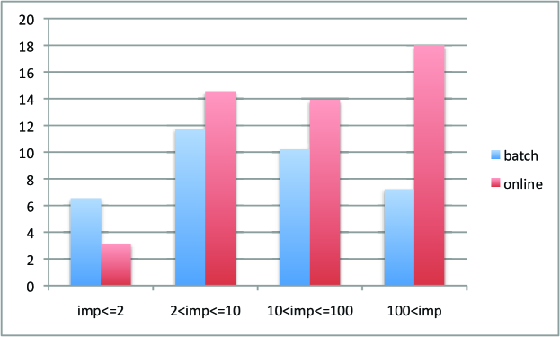
Figure 6: Relative CTR@1 lift in percentage ($\%$) over the baseline model (frmsc) for queries with different impressions.

Figure 7: Relative CTR@1 lift in percentage ($\%$) over the baseline model (frmsc) for queries with different lengths.

We now examine lift distribution over queries with different impression and lengths, respectively. Results of two representatives, batch(b) and online(b,ws), are reported.

Figure 6 presents CTR@1 lifts over frmsc aggregated over queries with different impressions. We notice that the online(b,ws) model is doing very well on popular recency queries, whereas the batch(b) model gives more lift on queries with less than 2 impressions. For queries with very limited impressions, e.g. less than 2, the online(b,ws) model cannot gain much advantage over the batch(b) model. This problem might be mitigated when applying the online(b,ws) model to larger traffic. This observation also suggests a practical solution, i.e. employing batch(b) models for queries with scarce impressions while using online(b,ws) models for popular recency queries only. It is expected that the online(b,ws) model achieves much more lift on popular recency queries, since the batch(b) model cannot specialize well on such cases despite the relatively large number of impressions. For example, the query “giant squids in California” was a popular recency query. A batch(b) model well trained on historical click events still fails to foresee the popularity and high relevance of the youtube video, whereas the online(b,ws) model does so correctly by adapting to users’ click feedback; see Section 5.4 for more details of this example.

Figure 7 presented CTR@1 lifts over frmsc for queries with different lengths. Except for a tie in two-word queries, the online(b,ws) model consistently outperforms the batch(b) model. The results suggest the online re-ranking method is robust to queries of various lengths.

5.3.3 Comparison of Other Click Metrics

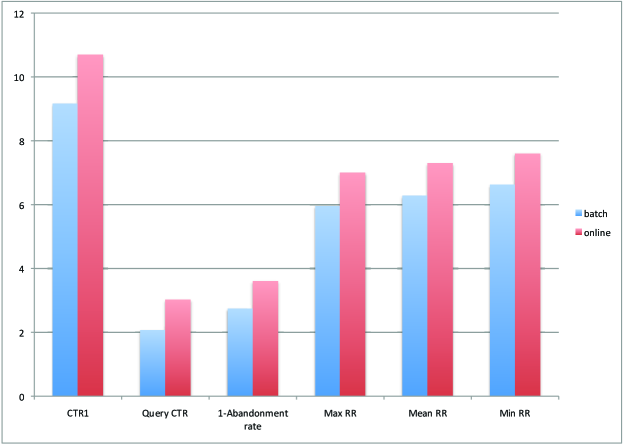
Figure 8: Relative lift in percentage ($\%$) over the baseline model (frmsc) on various click metrics.

(a) Zoom-in plot

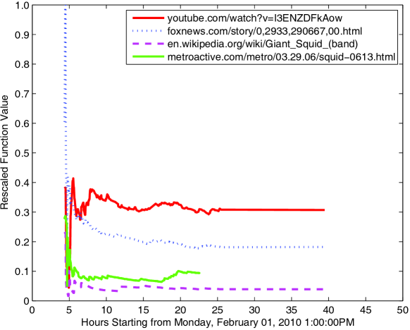
(b) Whole period

Figure 9: Function values in the online model on the 4 URLs associated with the recency query “giant squid in California”. Note that the URL of metroactive.com was replaced by another URL (not shown here) after the 23rd hour.

Although we have focused on training and evaluating our online re-ranking function based on CTR@1, we also compare our results with following other click metrics for ranking proposed in  [26]:

• Query CTR is the average number of clicks for each query

• $1-$Abandonment Rate is the probability of a session receiving a click

• Max RR (Reciprocal Rank) is the reciprocal rank of the highest ranked result clicked on

• Mean RR (Reciprocal Rank) is the average of clicked documents’ reciprocal ranks

• Min RR (Reciprocal Rank) is the reciprocal rank of the lowest ranked results clicked on.

Thus, for all metrics, higher values are assumed to indicate better ranking qualities.

In Figure 8, both batch and online models show significant lifts over the frmsc baseline on all click metrics listed above. Moreover, the online(b,ws) method consistently gives about 2% more lift than batch(b). Thus, although our algorithms focus on maximizing CTR@1, it also gives simultaneous lifts on other click metrics as well. This fact shows the easily measurable CTR@1 is a good surrogate to optimize, and also justifies our choice of using click at the top position as user feedback.

Ramark: We have done similar experiments on the non-recency queries as well, but our online re-ranking scheme did not show too much gain for those queries as in the recency queries, of which results are omitted here. The absence of improvements for non-recency queries is expected: the relevance of documents with respect to such queries does not change dramatically over time, so the re-ranking based on the click feedback may not be too different from the original ranking.

5.4 Case Study

We now revisit our example query “giant squid in California” in Section 3 to illustrate how our online re-ranking function can adapt to the click feedback quickly and track the best re-ranking. Coincidentally, the query happened to only appear in our test set. We ran our online model, online(b,ws), on the test set, and recorded the function values of the 4 URLs. Figure 9(a) shows the function values of 4 URLs for the first 10 hours, and Figure 9(b) presents the entire temporal curves for those function values in the lifetime of “giant squid in California”.

Since the initial re-ranking function online(b,ws) is (almost) identical to the fixed one of batch(b), we can see from Figure 9(a) that when the query appears around the 5th hour, batch(b) orders the four URLs as

1. foxnews.com/story/0,2933,290667,00.html

2. youtube.com/watch?v=I3ENZDFkAow

3. metroactive.com/metro/03.29.06/squid-0613.html

4. en.wikipedia.org/wiki/Giant_Squid_(band).

Note that this ranking is different from the frmsc ranking presented in Section 3. That is, although the batch(b) has not observed the query “giant squid in California” in its training set sessions, from the sessions of other queries in the training set, it was able to predict based on the query–document features that the “video” page will attract many clicks for the query and improve the original ranking. Nonetheless, we see that it still fails to accurately predict the users’ click behaviors.

On the other hand, given the users’ click patterns in Figure 4, the online(b,ws) promptly learns from them and put the “video” content with the highest CTR to the top rank within an hour. The ranking was then maintained for the rest of the time. Then, after the 25th hours, when the impression of the query quickly decreased toward 0 as shown in Figure 3, the function values of online(b,ws) were kept intact as can be seen in Figure 9(b).

Thus, this example indeed illustrates how re-ranking algorithms may benefit from user click feedback to improve ranking results. Furthermore, by real-time adaption online(b,ws) can quickly learn from users’ click patterns and outperforms not only the editorial-based batch recency ranking, frmsc, but also the click-based batch re-ranking, batch(b), for recency queries.

6 Related work

As mentioned in Section 1, the machine-learned ranking framework has been extended to the recency search problem. Previous work [8] introduced query classifiers to detect time-sensitive queries, implemented time-varying features that reflect document freshness, and recency demoted labels provided by human editors. More recently, improvements are made by introducing additional click related time-varying features [15, 9]. Algorithms studied in our work differ from them in two ways: (i) we use user click as training labels to gain further improvement; (ii) instead of fixing the ranking function and adjusting time-varying features, our features need not change over time, but the parameters of the ranking function can be automatically adjusted in real time based on user clicks.

Another related work [7] considered an online algorithm of slotting news direct display modules for recency queries in the search results page but did not consider re-rankings of documents.

Using users’ click feedback to improve ranking quality of a search engine has been extensively studied before. User behavior models (e.g., [10, 5, 14]) are developed based on click log data, whose outputs were then used as features for batch-training a ranking function. However, it is not easy to reflect temporal variations of document relevance in these works since the features were often computed in an average sense.

A few other works also used click data to directly modify their ranking based on the inference on the users’ relative preferences on rankings, but their settings or focuses are different: the method of [17] remained in the batch-learning mode and did not consider the temporal dimension of the click data; [25] was similar in spirit to ours but did not consider strategies that generalize to tail queries, and their results were based on simulated user clicks rather than real ones; finally, the dueling bandit approach [29] required a special functionality of the retrieval system to interleave two different ranking results.

Taking temporal variation of relevance into account to produce better rankings has also been considered in the past. [11] considered the temporal variations of document content and applied that knowledge to improve search ranking, but did not utilize click feedback to directly refine the ranking. [19] devised a scheme to capture temporal dynamics of user ratings on items in a collaborative filtering problem, but focused rather on long-term dynamics and did not consider the cold-start problem, which is critical to our recency ranking application give the large volume of of tail queries. Personalized article recommendation on web portals is another closely related problem. While models in earlier works (e.g., [1]) did not generalize, there have been efforts on generalization more recently, such as the LinUCB algorithm [21] that uses a similar linear model as ours, and the warm-start solution by [2]. However, both work remain to maintain models for a small number of articles/items, and so have not demonstrated capacities of learning with an almost infinitely large content pool, as in the space of query-document pairs in search domain. Another difference is that their model was more item-specific, whereas our model consists of both global model that applies to all queries and documents and specific bias term for each query-document pair. As a similar, independent thread of work, [28] also considered the large-scale personalized recommendation problem, but imposed a Bayesian framework, which is different from our work.

7 Conclusions

In this work, we investigated various learning algorithms to re-ranking recency search results based on real-time user feedback. Our contributions are three-fold. First, our evaluation method is novel for web search—a random exploration bucket was used to collect user feedback, which not only removed positional bias but also allowed one to reliably evaluate online learning algorithms offline. Second, we proposed a re-ranking approach to improve current search results for recency queries, and carried out extensive empirical results for a dozen of variants. Third, we demonstrated the need for using online learning as a flexible machine learning paradigm to adapt a ranking system to time-varying document relevance.

In future work, we would like to explore other options for correcting position biases and using clicks on multiple positions, e.g., using multiplicative bias correction terms or using user click models (e.g., [5]), so that we can effectively increase the size of training data and thus may result in faster learning speed in practice. In this work we focused on ranking documents based on individual document’s CTR estimate. It is also much more challenging to design algorithms for the best permutation of a set of documents, in which interactions between documents can be taken into account.

References

- [1] D. Agarwal, B. Chen, and P. Elango. Explore/exploit schemes for web content optimization. 2009. Proceedings of the International Conference on Data Mining (ICDM).
- [2] D. Agarwal, B. Chen, and P. Elango. Fast online learning through offline initialization for time-sensitive recommendation. 2010. ACM SIGKDD International Conference On Knowledge Discovery and Data Mining (KDD).
- [3] C. J. Burges, Q. V. Le, and R. Ragno. Learning to rank with nonsmooth cost functions. In B. Schölkopf, J. Platt, and T. Hofmann, editors, Advances in Neural Information Processing Systems (NIPS) 19, 2007.
- [4] C.J.C Burges, T. Shaked, E. Renshaw, A. Lazier, M. Deeds, N. Hamilton, and G. Hulldender. Learning to rank using gradient descent. In Proc. Intl. Conf. Machine Learning (ICML), 2005.
- [5] Olivier Chapelle and Ya Zhang. A dynamic bayesian network click model for web search ranking. In Proceedings of the 18th International World Wide Web (WWW) Conference, pages 1–10. ACM, 2009.
- [6] C. Cortes, M. Mohri, and A. Rastogi. Magnitude-preserving ranking algorithms. In Proceedings of the 24th International Conference on Machine Learning (ICML), 2007.
- [7] F. Diaz. Integration of news content into web results. 2009. Proceedings of the 2nd International ACM Conference on Web Search and Data Mining (WSDM).
- [8] A. Dong, Y. Chang, Zheng Z, G. Mishne, J. Bai, R. Zhang, K. Buchner, C. Liao, and F. Diaz. Towards recency ranking in web search. 2010. Proceedings of the 3rd International ACM Conference on Web Search and Data Mining (WSDM).
- [9] A. Dong, R. Zhang, P. Kolari, J. Bai, F. Diaz, Y. Chang, and Z. Zheng. Time is of the essence: Improving recency ranking using twitter data. 2010. Proceedings of the 19th International ACM Conference on World Wide Web (WWW).
- [10] Georges Dupret and Ciya Liao. Cumulated relevance: A model to estimate document relevance from the clickthrough logs of a web search engine. In Proceedings of the 3rd International ACM Conference on Web Search and Data Mining (WSDM), 2010.
- [11] Jonathan Elsas and Susan Dumais. Leveraging temporal dynamics of document content in relevance ranking. In Proceedings of the 3rd International Conference on Web Search and Data Mining (WSDM), 2010.
- [12] Y. Freund, R. Iyer, R.E. Schapire, and Y. Singer. An efficient boosting algorithm for combining preferences. Journal of Machine Learning Research, 4:933–969, 2003.
- [13] Thore Graepel, Joaquin Qui onero Candela, Thomas Borchert, and Ralf Herbrich. Web-scale Bayesian click-through rate prediction for sponsored search advertising in Microsoft’s Bing search engine. In Proceedings of the 27th International Conference on Machine Learning (ICML-10), pages 13–20, 2010.
- [14] F. Guo, C. Liu, A. Kannan, T. Minka, M. Taylor, Y. Wang, and C. Faloutsos. Click chain model in web search. In Proceedings of 18th International World Wide Web (WWW) Conference, 2009.
- [15] Y. Inagaki, N. Sadagopan, G. Dupret, C. Liao, A. Dong, Y. Chang, and Z. Zheng. Session based click features for recency ranking. 2010. Proceedings of the 24th AAAI Conference on Artificial Intelligence.
- [16] Kalervo Järvelin and Jaana Kekäläinen. Cumulated gain-based evaluation of ir techniques. ACM Transactions on Information Systems, 20:2002, 2002.
- [17] S. Ji, K. Zhao, C. Liao, Z. Zheng, G. Xue, O. Chapelle, G. Sun, and H. Zha. Global ranking by exploiting user clicks. In Proceedings of the 28th International ACM SIGIR conference, pages 35–42, 2009.
- [18] Thorsten Joachims. Optimizing search engines using clickthrough data. In Proceedings of the 8th ACM SIGKDD International Conference on Knowledge Discovery and Data Mining (KDD), pages 133–142, New York, NY, USA, 2002. ACM Press.
- [19] Y. Koren. Collaborative filtering with temporal dynamics. 2009. ACM SIGKDD International Conference On Knowledge Discovery and Data Mining (KDD).
- [20] J. Langford, L. Li, and A. Strehl. Vowpal wabbit online learning project, 2007. http://hunch.net/?p=309.
- [21] L. Li, W. Chu, J. Langford, and R. Schapire. A contextual bandit approach to personalized news article recommendation. 2010. Proceedings of 19th World Wide Web (WWW) Conference.
- [22] Lihong Li, Wei Chu, John Langford, and Xuanhui Wang. Unbiased offline evaluation of contextual-bandit-based news article recommendation algorithms. In Proceedings of the 4th International Conference on Web Search and Web Data Mining (WSDM), 2011.
- [23] T. Y. Liu. Learning to Rank for Information Retrieval. Now Publishers, 2009.
- [24] T. Moon, L. Li, W. Chu, C. Liao, Z. Zheng, and Y. Chang. Online learning for recency search ranking using real-time user feedback. 2010. Proceedings of the 19th International Conference on Knowledge Management (CIKM).
- [25] F. Radlinski and T. Joachims. Active exploration for learning rankings from clickthrough data. 2007. ACM SIGKDD International Conference On Knowledge Discovery and Data Mining (KDD).
- [26] F. Radlinski, Madhu Kurup, and T. Joachims. How does clickthrough data reflect retrieval quality? 2008. Proceedings of 17th ACM Conference on Information and Knowledge Management (CIKM).
- [27] Herbert Robbins. Some aspects of the sequential design of experiments. Bulletin of the American Mathematical Society, 58(5):527–535, 1952.
- [28] David Stern, Ralf Herbrich, and Thore Graepel. Matchbox: Large scale online bayesian recommendations. In Proceedings of the 18th International World Wide Web (WWW) Conference, 2009.
- [29] Y. Yue and T. Joachims. Interactively optimizing information retrieval systems as a dueling bandits problem. 2009. Proceedings of the 26th International Conference on Machine Learning (ICML).
- [30] Z. Zheng, H. Zha, T. Zhang, O. Chapelle, and K. Chen. A general boosting method and its application to learning ranking functions for web search. In Advances in Neural Information Processing Systems (NIPS) 20. MIT Press, Cambridge, MA, 2008.