Extended self-energy functional approach for strongly-correlated lattice bosons
in the superfluid phase

Abstract

Among the various numerical techniques to study the physics of strongly correlated quantum many-body systems, the self-energy functional approach (SFA) has become increasingly important. In its previous form, however, SFA is not applicable to Bose-Einstein condensation or superfluidity. In this paper we show how to overcome this shortcoming. To this end we identify an appropriate quantity, which we term $D$, that represents the correlation correction of the condensate order parameter, as it does the self-energy for the Green’s function. An appropriate functional is derived, which is stationary at the exact physical realizations of $D$ and of the self-energy. Its derivation is based on a functional-integral representation of the grand potential followed by an appropriate sequence of Legendre transformations. The approach is not perturbative and therefore applicable to a wide range of models with local interactions. We show that the variational cluster approach based on the extended self-energy functional is equivalent to the “pseudoparticle” approach introduced in Phys. Rev. B, 83, 134507 (2011). We present results for the superfluid density in the two-dimensional Bose-Hubbard model, which show a remarkable agreement with those of Quantum-Monte-Carlo calculations.

I Introduction

Seminal experiments with ultracold gases of atoms trapped in optical lattices shed new light on strongly-correlated many body systems.Jaksch et al. (1998); Greiner et al. (2002); Bloch et al. (2008) In these experiments specific lattice Hamiltonians can be engineered and investigated with a remarkable high level of control, making quantum mechanical interference effects observable on a macroscopic scale. Most important as well as fundamental is the quantum phase transition of strongly correlated lattice bosons from the localized Mott phase to the delocalized superfluid phase. In the superfluid phase a macroscopic fraction of the particles condenses into one quantum mechanical state, thus, forming a Bose-Einstein condensate, where the number of particles in the condensate is not necessarily equal to the number of superfluid particles. In experiments with ultracold gases of atoms trapped in optical lattices, the condensate density can be extracted from time-of-flight images,Greiner et al. (2002) which are related to the momentum distribution of the confined particles. Importantly, the finite expansion time of the particle cloud has to be taken into account when drawing the connection between these time-of-flight images and the true momentum distribution.Gerbier et al. (2008); Trotzky et al. (2010); Kato et al. (2008); Diener et al. (2007) However, it is probably even more challenging to measure the superfluid density itself, as it is not a ground state property but rather related to the response of the system to a phase twisting field.Roth and Burnett (2003) Interestingly, only very recently for Bose gases without the periodic lattice potential an optical method has been proposed to extract the superfluid density. This experiment creates a vector potential, that imposes angular momentum on normal fluid particles, while superfluid particles stay at rest.Cooper and Hadzibabic (2010)

In a previous work, we extended the variational cluster approach (VCA), which is capable to deal with strongly-correlated many body systems without broken symmetry to the superfluid phase of lattice bosons.Knap et al. (2011) Originally, VCA has been formulated for the normal Mott phase of lattice bosons in Ref. Koller and Dupuis, 2006 within the so-called self-energy functional approach (SFA), which was previously introduced for interacting fermionic systems.Potthoff (2003a, b) Our extension to the superfluid phase in Ref. Knap et al., 2011 follows a different path, and is based on the so-called “pseudoparticle” formalism. Within this approach we obtained the expressions for the superfluid order parameter, the anomalous Green’s function, and the grand potential, which is the starting point for the variational principle, see Eq. (1), (33), and (2) in this reference.

It should be pointed out that, while the pseudoparticle formalism is equivalent to VCA in the normal phase of both bosonic Knap et al. (2011) and fermionic Zacher et al. (2002) systems, it lacks the rigorous theroretical framework provided by SFA. In particular, there is no genuine variational principle explaining why one should look for a saddle point in the grand potential. The goal of the present paper is to put the results obtained within the pseudoparticle approach into a rigorous framework by developing an extended self-energy functional approach, which is capable to deal with the bosonic superfluid phase.

From the present work it will become clear, that this extension is not straightforward, as it involves a precise sequence of Legendre transformations with suitably chosen variables. In the search for the appropriate set of transformations the knowledge of the final results provided by pseudoparticle formalism proves to be useful. This fact emphasizes the advantage of the heuristic, yet straightforward, pseudoparticle approach to formulate extensions of VCA.Knap et al. (2011)

The extended SFA formulated in the present paper yields the same expressions for the superfluid order parameter, for the Nambu Green’s function, and for the grand potential, as obtained from the pseudoparticle approach. While this might not seem to be surprising, since we were guided by the very results of the pseudoparticle approach, we argue below, that our SFA extension presented here is unambiguous. The most important step in this SFA extension is to find a quantity, which we call $D$, which is the companion of the self-energy in the superfluid phase. Correspondingly, one has to find an appropriate universal functional of this quantity and of the self-energy, which generates the superfluid order parameter and the Green’s function.

As an application, we present an evaluation of the superfluid density within this extended VCA, by the usual method of introducing a phase twisting field, which is equivalent to the helicity modulusFisher et al. (1973) and to winding numbers in quantum Monte Carlo (QMC) algorithms.Pollock and Ceperley (1987); Prokof’ev and Svistunov (2000) We evaluate the superfluid density for the two-dimensional Bose-Hubbard (BH) modelFisher et al. (1989) and find a remarkably excellent agreement with QMC results.

This article is organized as follows. In Sec. II we extend SFA to the superfluid phase and obtain the corresponding extended self-energy functional, along with the appropriate variable describing superfluidity. The evaluation of the superfluid density within this extended VCA is presented in Sec. III and applied to the BH model in two dimensions. The VCA results are compared with unbiased QMC results showing excellent agreement. Finally, we conclude and summarize our findings in Sec. IV.

II Self-energy functional approach

Let us recall the key idea of SFA due to M. Potthoff. Potthoff (2003a) The starting point is an appropriate functional

$$\hat{\Omega}[\Sigma,G_{0}^{-1},H_{U}] \equiv\hat{\cal F}[\Sigma,H_{U}]+\hat{\cal E}[\Sigma,G_{0}^{-1}]\;,$$ (1)

which consists of a functional $\hat{\cal F}$ of the self-energy, the Legendre transform of the Luttinger-Ward functional, which is universal in the sense that it depends on the interaction part ($H_{U}$) of the Hamiltonian but not on the single particle part. The latter enters via the free Green’s function $G_{0}^{-1}$ in the second functional, which is explicitly known

$$\hat{\cal E}[\Sigma,G_{0}^{-1}] \equiv-\beta\operatorname{\mbox{tr}}\ln(\Sigma-G_{0}^{-1})$$

The functional $\hat{\Omega}[\Sigma,G_{0}^{-1},H_{U}]$ has three key features, which are crucial for VCA.

• The non-universal part $\hat{\cal E}$ enters additively in form of a known functional and the many-body aspects are described by a universal functional independent of the single particle Hamiltonian, or, equivalently, independent of $G_{0}^{-1}$.

• The self-energy of the physical system, characterized by $H_{U}$ and $G_{0}^{-1}$ is a stationary point of the functional $\hat{\Omega}$ with respect to $\Sigma$.

• The value of $\hat{\Omega}$ at the stationary point is equal to the thermodynamic grand potential.

Given these properties, one can construct a parametric family of Hamilton operators based on the same interaction part (reference systems), for which the thermodynamic grand potential, the Green’s function and the self-energy can be determined exactly. This allows to determine the exact self-energy functional for self-energies accessible by the reference systems. In this very subspace, the self-energy functional in Eq. (1) for the physical system is replaced by that of the reference system. The stationarity condition in turn allows to determine the Green’s function and self-energy of the physical system.

Our goal is to generalize this approach to the superfluid phase as well. Besides the self-energy, which is the interaction correction of the inverse Green’s function, we need the corresponding companion that describes the interaction correction to the order parameter, which we call $D$.

Once the appropriate form of $D$ has been determined, we need a functional

$${\hat{\Omega}}_{s}[\Sigma,D,F,G_{0}^{-1},H_{U}] \equiv\hat{\cal F}[\Sigma,D,H_{U}]+\hat{\cal E}[\Sigma,D,G_{0}^{-1},F]\;,$$

in the self-energy $\Sigma$ and $D$ with the following features.

• $\hat{\cal F}$ is again a universal functional, now in $\Sigma$ and $D$. The non-universal part $\hat{\cal E}$ is explicitly known and carries the dependence on $G_{0}^{-1}$ and the symmetry breaking source-field $F$.

• The functional is again stationary at the exact self-energy $\Sigma$ and the exact $D$ of the physical system, characterized by $H_{U}$, $G_{0}^{-1}$ and $F$.

• The value of ${\hat{\Omega}}_{s}$ at the stationary point is equal to the thermodynamic grand potential.

The sought-for functional ${\hat{\Omega}}_{s}$, to be derived in this section, will turn out to be (see below for a definition of the quantities)

$$2\beta{\hat{\Omega}}_{s}[\Sigma,\,D,G_{0}^{-1},F] =\hat{\cal F}[\Sigma,D]+\hat{\cal E}[\Sigma,\,D,G_{0}^{-1},F]$$ (2)

$$\hat{\cal E}[\Sigma,\,D,G_{0}^{-1},F] \equiv{\beta}\operatorname{\mbox{Tr}}\ln[{({G_{0}^{-1}}-\Sigma)\ G_{\infty}}]$$

$$+(\bar{D}-\bar{F})(G_{0}^{-1}-\Sigma)^{-1}(D-F)\;.$$ (3)

In the normal phase, it is identical to the functional introduced by Potthoff. The additional factor 2 is due to the Nambu Green’s functions. Moreover, the expression for the grand potential obtained with the help of a so-called reference system, see Eq. 30 below, is identical to the one obtained within the pseudoparticle approach. Knap et al. (2011)

II.1 Derivation of the grand potential functional

We start out from the partition function $Z$ of a bosonic many-body system, which in a functional integral representation reads

$$Z=\int\mathcal{D}A\;e^{-S}\;,$$ (4)

where $S$ is the action, which in general can be written assym

$$S= -\frac{1}{2}\int d\tau\int d\tau^{\prime}\,\bar{A}(\tau^{\prime})\,G_{0}^{-1}(\tau^{\prime},\tau)\,A(\tau)$$

$$-\int d\tau\left[\bar{F}(\tau)\,A(\tau)-H_{U}(A(\tau))\right]\;.$$ (5)

In view of treating the superfluid phase we have adopted a Nambu notation in which the bosonic fields are expressed in a vector representation

$$A(\tau)\equiv\left(\begin{array}[]{c}a_{1}(\tau)\\ \vdots\\ a_{N}(\tau)\\ \bar{a}_{1}(\tau)\\ \vdots\\ \bar{a}_{N}(\tau)\end{array}\right)\;.$$ (6)

The indices $1$ through $N$ denote the corresponding single-particle orbitals (for example, lattice sites) where the boson operators act, and $a_{i}(\tau)$ ($\bar{a}_{i}(\tau)$) are the fields associated with the annihilation (creation) of a boson in the orbital $i$. The adjoint field is defined as

$$\bar{A}(\tau)\equiv\left(\bar{a}_{1}(\tau),\\ \cdots,\\ \bar{a}_{N}(\tau),a_{1}(\tau),\\ \cdots,\\ a_{N}(\tau)\right)\;.$$ (7)

It can be expressed in terms of $A(\tau)$ with the help of the matrix ${\cal T}$, which exchanges the first $N$ entries of a vector with the last $N$ ones:

$$\bar{A}(\tau)=A(\tau)^{T}{\cal T}\;.$$ (8)

The operator ${\cal T}$ has the properties ${\cal T}^{2}=\mathbbm{1}$, and ${\cal T}={\cal T}^{T}$. The action in Eq. (5) also contains the source fields

$$\bar{F}\equiv\left(f_{1},\cdots f_{N},\bar{f}_{1},\cdots,\bar{f}_{N}\right)\quad\text{and}\quad F={\cal T}\bar{F}^{T}\;,$$

which are zero for the physical system of interest, the boson interaction described by $H_{U}$, as well as the $2N\times 2N$ noninteracting Green’s function matrix $G_{0}(\tau^{\prime},\tau)$. Eq. (4) with Eq. (5) defines the corresponding grand potential as a functional of $G_{0}^{-1}$ and $F$

$$\hat{\widetilde{\Omega}}_{s}[G_{0}^{-1},F]\equiv-\frac{1}{\beta}\ln{\hat{Z}}\,,$$ (9)

where $\beta$ is the inverse temperature. Here and in the following, we mark functionals with a hat “$\hat{\phantom{\cdots}}$”, and omit their arguments whenever they are obvious. The noninteracting Green’s function has the matrix structure (see App. A.3)

$${G}_{0}^{-1}(\tau^{\prime},\,\tau)=-\delta(\tau-\tau^{\prime})\left(\begin{array}[]{cc}\partial_{\tau}+\mathsf{{{\bf t}}}&0\\ 0&-\partial_{\tau}+\mathsf{{{\bf t}}}\end{array}\right)\;,$$ (10)

where ${{\bf t}}$ is the single-particle Hamiltonian matrix.

In the following, we carry out a sequence of Legendre transformations starting from $\hat{\widetilde{\Omega}}_{s}$, ultimately leading to a universal functional $\hat{\cal F}[\Sigma,D]$ of the self-energy $\Sigma$ and of a suitable quantity $D$ defined in Eq. (21a). The functional $\hat{\cal F}$ is the generalization of the self-energy functional Potthoff (2003a, b); Koller and Dupuis (2006) to the superfluid phase, where a nonvanishing expectation value $\mathcal{A}(\tau){\equiv}\langle A(\tau)\rangle$ of the boson operators $A$ exists. The functional $\hat{\cal F}$ has the properties, see Eq. (23), that its functional derivatives with respect to $\Sigma$ and $D$ yield the disconnected Green’s function, and the expectation value $\mathcal{A}$, respectively. This procedure is inspired by Ref. Potthoff, 2006 and extends that approach to the treatment of the superfluid phase.

We first determine the conjugate variables to $G_{0}^{-1}$ and to the source fields $F$. The functional derivative of $\hat{\widetilde{\Omega}}_{s}$ with respect to the noninteracting Green’s function yieldssym (see App. A.1)

$$2\beta\frac{\delta\hat{\widetilde{\Omega}}_{s}}{\delta{G_{0\,ji}^{-1}}(\tau^{\prime},\tau)}=-\frac{2}{\hat{Z}}\frac{\delta}{\delta{G_{0\,ji}^{-1}}(\tau^{\prime},\tau)}\int\mathcal{D}A\times$$

$$\quad\quad\times\exp\Big{\{}\frac{1}{2}\int d\tilde{\tau}\int d\tilde{\tau}^{\prime}\bar{A}_{l}(\tilde{\tau})\,G_{0\,ll^{\prime}}^{-1}(\tilde{\tau},\tilde{\tau}^{\prime})\,A_{l^{\prime}}^{\phantom{\dagger}}(\tilde{\tau}^{\prime})$$

$$\quad\quad+\int d\tilde{\tau}[\bar{F}_{l}(\tilde{\tau})\,A_{l}^{\phantom{\dagger}}(\tilde{\tau})-H_{U}(\bar{a},\,a)]\Big{\}}$$

$$\quad=-\frac{1}{\hat{Z}}\int\mathcal{D}A\,{\bar{A}_{j}(\tau^{\prime})\,A_{i}^{\phantom{\dagger}}(\tau)\exp\left[-S\right]}$$

$$\quad\equiv\operatorname{{\hat{G}_{disc}}}_{,ij}(\tau,\tau^{\prime})\;.$$

Here $\operatorname{{\hat{G}_{disc}}}_{,ij}(\tau,\tau^{\prime})$ is the disconnected interacting time-ordered Green’s function. Along with the definition of the connected Green’s function $\hat{G}[G_{0}^{-1},F]$ we obtain

$$2\beta\frac{\delta\hat{\widetilde{\Omega}}_{s}[G_{0}^{-1},F]}{\delta G_{0}^{-1}} =\operatorname{{\hat{G}_{disc}}}\equiv\hat{G}-\hat{\mathcal{A}}\hat{\bar{\mathcal{A}}}\;.$$ (11a)

For the functional derivative with respect to $$F$$ we obtain similarly

$$2\beta\frac{\delta\hat{\widetilde{\Omega}}_{s}[G_{0}^{-1},F]}{\delta\bar{F}} =-2\hat{\mathcal{A}}[G_{0}^{-1},F]\;.$$ (11b)

The two functionals $\hat{G}[G_{0}^{-1},F]$ and $\hat{A}[G_{0}^{-1},F]$ defined in Eq. (11) provide the exact Green’s function $G$ and order parameter $A$ for a given noninteracting Green’s function $G_{0}^{-1}$ and source field $F$ of the system. The first step toward the universal functional consists in a Legendre transformation replacing the variables $F$ with $\mathcal{A}$. To this end, we invert inv the relation Eq. (11) making $F$ a functional $\hat{F}[G_{0}^{-1},\mathcal{A}]$ and introduce

$$\hat{\Xi}[G_{0}^{-1},\,\mathcal{A}]=2\beta\hat{\widetilde{\Omega}}_{s}+2\hat{\bar{F}}\mathcal{A}\;,$$ (12)

where, as usually in Legendre transformations, the functional dependence on $F$ has been eliminated in favor of $\mathcal{A}$ by using the inverse function. It is straightforward to show that the corresponding functional derivatives give

$$\frac{\delta\hat{\Xi}}{\delta 2\mathcal{A}}=\hat{\bar{F}}[G_{0}^{-1},A]\;,\quad\frac{\delta\hat{\Xi}}{\delta{G_{0}^{-1}}}=\operatorname{{\hat{G}_{disc}}}[G_{0}^{-1},A]\;.$$

Next, we modify the functional in the following way

$$\hat{\widetilde{\Xi}}[G_{0}^{-1},\,\mathcal{A}]=\hat{\Xi}+\bar{\mathcal{A}}G_{0}^{-1}\mathcal{A}\;,$$ (13)

such that we obtain the connected Green’s function from the functional derivative with respect to $G_{0}^{-1}$. In total we have

$$\frac{\delta\hat{\widetilde{\Xi}}}{\delta 2\mathcal{A}} =\hat{\bar{F}}[G_{0}^{-1},A]+\bar{\mathcal{A}}G_{0}^{-1}\;,$$ (14)

$$\frac{\delta\hat{\widetilde{\Xi}}}{\delta{G_{0}^{-1}}} =\operatorname{{\hat{G}_{disc}}}+\mathcal{A}\bar{\mathcal{A}}=\hat{G}[G_{0}^{-1},A]\;.$$ (15)

The second step is a Legendre transformation replacing the variable $G_{0}^{-1}$ with $G$

$$\hat{\Pi}[G,\,\mathcal{A}]=\hat{\widetilde{\Xi}}-{\beta}\operatorname{\mbox{Tr}}(G\,\hat{G}_{0}^{-1}-\mathbbm{1})\;,$$ (16)

where we have expressed $\hat{G}_{0}^{-1}$ as a functional of $G$ and $\mathcal{A}$, by inverting Eq. (15).inv ; sym We subtract an “infinite” constant ${\beta}\operatorname{\mbox{Tr}}\mathbbm{1}$ in order to keep $\hat{\Pi}[G,\,\mathcal{A}]$ finite. The functional derivatives of the new functional are

$$\frac{\delta\hat{\Pi}}{\delta 2\mathcal{A}}=\hat{\bar{F}}+\bar{\mathcal{A}}\hat{G}_{0}^{-1}\;,\quad\frac{\delta\hat{\Pi}}{\delta G}=-\hat{G}_{0}^{-1}\;.$$

Now, we modify the functional such that we get the self-energy from the functional derivative (see App. A.1.3)

$$\hat{\widetilde{\Pi}}[G,\,\mathcal{A}]=\hat{\Pi}+{\beta}\operatorname{\mbox{Tr}}\ln\left(G/G_{\infty}\right)\;.$$ (17)

This gives

$$\frac{\delta\hat{\widetilde{\Pi}}}{\delta 2\mathcal{A}} =\hat{\bar{F}}+\bar{\mathcal{A}}\hat{G}_{0}^{-1}\;,\quad\frac{\delta\hat{\widetilde{\Pi}}}{\delta G}=\hat{\Sigma}$$ (18a)

$$\hat{\Sigma} \equiv G^{-1}-\hat{G}_{0}^{-1}\;.$$ (18b)

Here we have used the Dyson equation as defining equation for the self-energy. Furthermore, we carry out a third Legendre transformation replacing $G$ with $\Sigma$ in the usual way. Thus we introduce

$$\hat{P}[\Sigma,\,\mathcal{A}]=\hat{\widetilde{\Pi}}+{\beta}\operatorname{\mbox{Tr}}\Sigma\,\hat{G}\;$$ (19)

with the properties

$$\frac{\delta\hat{P}}{\delta 2\mathcal{A}}=\hat{\bar{F}}+\bar{\mathcal{A}}\hat{G}_{0}^{-1}\;,\quad\frac{\delta\hat{P}}{\delta\Sigma}=\hat{G}\;.$$

We modify this functional once more so that its derivative yields a new function $D$, which will be the companion of the self-energy in our extended self-energy approach

$$\hat{\widetilde{P}}[\Sigma,\,\mathcal{A}]=\hat{P}-\bar{\mathcal{A}}\Sigma\mathcal{A}\;.$$ (20)

The functional derivatives yield

$$\frac{\delta\hat{\widetilde{P}}}{\delta 2\mathcal{A}} =\hat{\bar{F}}+\bar{\mathcal{A}}\hat{G}_{0}^{-1}-\bar{\mathcal{A}}\Sigma=\hat{\bar{F}}+\bar{\mathcal{A}}\hat{G}^{-1}\equiv\hat{\bar{D}}\;,$$ (21a)

$$\frac{\delta\hat{\widetilde{P}}}{\delta\Sigma} =\hat{G}-\mathcal{A}\bar{\mathcal{A}}={\hat{G}_{\text{disc}}}\;.$$ (21b)

Before proceeding, let us discuss the meaning of the function $D$ introduced in Eq. (21a). When extending SFA to the superfluid phase one is looking for a quantity, which is related to the condensed order parameter and which plays a similar role as the self-energy, in that it describes the deviation between the interacting and non-interacting case. Thus, this quantity should vanish in the noninteracting case ($H_{U}=0$). The reason is that SFA will eventually amount to an approximation for $\Sigma$ and $D$, and we require this approximation to become exact for $H_{U}=0$. Finally, $D$ must obviously vanish in the normal phase. The expression in Eq. (21a) has precisely these features, since $\bar{\mathcal{A}}_{0}=-\bar{F}G_{0}$, which is straightforwardly determined from the Gaussian integral for $H_{U}=0$ in Eq. (5). Interestingly, the pseudoparticle approach, presented in Ref. Knap et al., 2011, and which is based on an intuitive, yet heuristic approximation, provides the same form of $D$ as given in Eq. (21a).

The final Legendre transformation replacing $\mathcal{A}$ with $D$ yields the desired functional of the self-energy and $D$. It represents the generalization of the self-energy functional ($F[\Sigma]$ of Refs. Potthoff, 2003a and Koller and Dupuis, 2006) to the superfluid phase

$$\hat{\cal F}[\Sigma,\,D]=\hat{\widetilde{P}}-2\bar{D}\hat{\mathcal{A}}\;$$ (22)

and has the properties

$$\frac{\delta\hat{{\cal F}}}{\delta\bar{D}}=-2\hat{\mathcal{A}}[\Sigma,D]\;,\quad\frac{\delta\hat{{\cal F}}}{\delta\Sigma}=\operatorname{{\hat{G}_{disc}}}[\Sigma,D]\;.$$ (23)

Similarly to $F[\Sigma]$ from Refs. Potthoff, 2003a and Koller and Dupuis, 2006, $\hat{\cal F}$ is (for fixed $H_{U}$) a universal functional of $\Sigma$ and $D$ only, from which the disconnected Green’s function and the order parameter are obtained by functional derivative, see Eq. (23).

Given $\Sigma$ and $D$ we can compute by Eq. (23) the corresponding values for $A$ and $\operatorname{{G_{disc}}}$. On the other hand, for a specific physical system, uniquely defined by $G_{0}^{-1}$, $F$ and $H_{U}$, the definitions of the self-energy $\Sigma$, Eq. (18b), and the modified order parameter $D$, Eq. (21a), provide another set of equations, which uniquely fix $\Sigma$ and $D$ via the equations

$${\operatorname{{\hat{G}_{disc}}}[\Sigma,D]} \overset{!}{=}(G_{0}^{-1}-\Sigma)^{-1}+$$ (24a)

$$(G_{0}^{-1}-\Sigma)^{-1}(D-F)(\bar{D}-\bar{F})(G_{0}^{-1}-\Sigma)^{-1}\;,$$

and

$${-2\bar{\mathcal{A}}[\Sigma,D]} \overset{!}{=}-2(\bar{D}-\bar{F})(G_{0}^{-1}-\Sigma)^{-1}\;.$$ (24b)

As for the (original) self-energy functional approach, we seek now a functional, which becomes stationary at the exact $\Sigma$ and $D$ for specific $G_{0}^{-1}$ and $F$, and which consists of the universal functional $\hat{\cal F}$ plus a non-universal explicit functional of the form

$$2\beta{\hat{\Omega}}_{s}[\Sigma,D,G_{0}^{-1},F,H_{U}] =\hat{\cal F}[\Sigma,D,H_{U}]+\hat{\cal E}[\Sigma,D,G_{0}^{-1},F]\;.$$

In order to yield the correct stationary point, the functional $\hat{\cal E}$ has to fulfill according to Eq. (24) the equations

$$\frac{\delta\hat{\cal E}}{\delta\Sigma}= -(G_{0}^{-1}-\Sigma)^{-1}$$ (25a)

$$-(G_{0}^{-1}-\Sigma)^{-1}(D-F)(\bar{D}-\bar{F})(G_{0}^{-1}-\Sigma)^{-1}\;,$$

$$\frac{\delta\hat{\cal E}}{\delta D} =2(\bar{D}-\bar{F})(G_{0}^{-1}-\Sigma)^{-1}\;.$$ (25b)

With these ingredients we can now express the sought-for functional ${\hat{\Omega}}_{s}$ as

$$2\beta{\hat{\Omega}}_{s}[\Sigma,\,D,G_{0}^{-1},F] =\hat{\cal F}[\Sigma,D]+{\beta}\operatorname{\mbox{Tr}}\ln[{({G_{0}^{-1}}-\Sigma)\ G_{\infty}}]$$

$$+(\bar{D}-\bar{F})(G_{0}^{-1}-\Sigma)^{-1}(D-F)\;,$$ (26)

which obviously fulfills Eq. (25). It remains to show that, whenever evaluated at the exact $\Sigma$ and $D$ the functional ${\hat{\Omega}}_{s}$ corresponds, possibly apart from a constant, to the thermodynamic grand potential ${\widetilde{\Omega}}_{s}$ of the system. To this end we add up all the terms used to construct the functional. At the exact values of $\Sigma$ and $D$ we have

$$2\beta{{\hat{\Omega}}_{s}}\bigl{|}_{exact} = 2 \beta{\widetilde{\Omega}}_{s}+2\bar{F}\mathcal{A}+\bar{\mathcal{A}}G_{0}^{-1}\mathcal{A}-{\beta}\operatorname{\mbox{Tr}}\left(GG_{0}^{-1}-\mathbbm{1}\right)$$

$$+ {\beta}\operatorname{\mbox{Tr}}\ln\left(G/G_{\infty}\right)+{\beta}\operatorname{\mbox{Tr}}\Sigma G-\bar{\mathcal{A}}\Sigma\mathcal{A}-2\bar{D}\mathcal{A}$$

$$- {\beta}\operatorname{\mbox{Tr}}\ln\left(G/G_{\infty}\right)+\bar{\mathcal{A}}G^{-1}\mathcal{A}$$

$$= 2 \beta{\widetilde{\Omega}}_{s}-2\underbrace{(\bar{D}-\bar{F})}_{\bar{\mathcal{A}}G^{-1}}\mathcal{A}+2\bar{\mathcal{A}}G^{-1}\mathcal{A}$$

$$= 2 \beta{\widetilde{\Omega}}_{s}$$

We can now proceed as in Refs. Potthoff, 2003a and Potthoff et al., 2003 and construct a reference system, which can be solved (almost) exactly.cut The reference system is described by a Hamiltonian $H^{\prime}$, which shares the same interaction $H_{U}$ as the physical system, but consists of different noninteracting Green’s function $G_{0}^{\prime}$ and source fields $F^{\prime}$. The point is the following: Due to the fact that ${\cal F}$ is a universal functional, it cancels out from the difference between ${\hat{\Omega}}_{s}$ for the physical and the reference system, with the same values of $\Sigma$ and $D$. In particular, this gives

$$2\beta{\hat{\Omega}}_{s}[\Sigma,D,G_{0}^{-1},F]-2\beta{\hat{\Omega}}_{s}[\Sigma,D,G_{0}^{\prime-1},F^{\prime}]\\ ={\beta}\operatorname{\mbox{Tr}}\ln\left((G_{0}^{-1}-\Sigma)G_{\infty}\right)-{\beta}\operatorname{\mbox{Tr}}\ln\left((G_{0}^{\prime-1}-\Sigma)G_{\infty}\right)\\ +(\bar{D}-\bar{F})(G_{0}^{-1}-\Sigma)^{-1}(D-F)\\ -(\bar{D}-\bar{F}^{\prime})(G_{0}^{\prime-1}-\Sigma)^{-1}(D-F^{\prime})\;,$$ (27)

which allows to evaluate the functional ${\hat{\Omega}}_{s}$ exactly for the physical system as well, however, in a restricted subspace of $\Sigma$ and $D$, representable by the parametric family of reference systems. By construction, the optimal values for $\Sigma$ and $D$ for the physical system are those of the reference system for the set of optimal variational parameters.

The variational procedure then follows and generalizes Ref. Potthoff, 2003a: First a class of exactly solvable reference systems $\hat{H}^{\prime}$ with the same interaction as the physical system characterized by a continuum of single-particle parameters ${{\bf t}}^{\prime}$ and source fields $F^{\prime}$ is identified. In VCA this class is obtained by dividing the original lattice into disconnected clusters with varying single-particle energies and hopping strengths. A larger subspace can be reached by adding bath sites. Potthoff (2003b) Then the (connected) Green’s function $G^{\prime}$, the order parameter $\mathcal{A}^{\prime}$, and the grand potential $\Omega_{s}^{\prime}$ of the reference system is evaluated. With the help of Dyson’s equation Eq. (18b) the self-energy $\Sigma^{\prime}$, and with the help of Eq. (21a) $D^{\prime}$ is determined. By varying ${{\bf t}}^{\prime}$ and $F^{\prime}$ the subspace of self-energies and $D$s is spanned, which is accessible to the reference system and to which these objects for the physical system are restricted. Within this subspace the functional ${\hat{\Omega}}_{s}$ can be evaluated exactly for arbitrary $G_{0}$ and $F$ of the physical system. For the relevant case $F=0$ we obtain nog from Eq. (27)

$$2\beta\Omega_{s} =2\beta\Omega_{s}^{\prime}+{\beta}\operatorname{\mbox{Tr}}\ln\left(-(G_{0}^{-1}-\Sigma^{\prime})\right)$$

$$-{\beta}\operatorname{\mbox{Tr}}\ln\left(-(G_{0}^{\prime-1}-\Sigma^{\prime})\right)+\bar{D}(G_{0}^{-1}-\Sigma^{\prime})^{-1}D$$

$$-\bar{\mathcal{A}}^{\prime}G^{\prime-1}\mathcal{A}\;,$$ (28)

which is now a function of ${{\bf t}}^{\prime}$ and $F^{\prime}$. The infinite physical system can break the symmetry spontaneously, while in the reference systems of disconnected finite clusters, a non-vanishing order parameter can only be achieved by an additional source field $F^{\prime}$. This explains, why a finite $F^{\prime}$ is required although $F=0$ in the physical system. The SFA approximation consists in finding a stationary point of ${\hat{\Omega}}_{s}$ within this subspace of self-energies and $D$-s. This corresponds, quite generally, to finding a stationary point with respect to ${{\bf t}}^{\prime}$ and $F^{\prime}$ of Eq. (28), i. e. to the equations

$$\frac{\partial\Omega}{\partial{{\bf t}}^{\prime}}=0\quad\quad\frac{\partial\Omega}{\partial F^{\prime}}=0\;.$$ (29)

Here, we have replaced $\Omega_{s}$ with $\Omega\equiv\Omega_{s}-\frac{1}{2}\operatorname{\mbox{tr}}{{\bf t}}$ which differs just by a ${{\bf t}}^{\prime}$- and $F^{\prime}$-independent constant and thus does not change the saddle-point equations. The quantity $\Omega$ is the grand potential obtained from the normal-ordered Hamiltonian (see App. A.3). We also introduce the grand-potential of the normal-ordered reference system $\Omega^{\prime}\equiv\Omega_{s}^{\prime}-\frac{1}{2}\operatorname{\mbox{tr}}{{\bf t}}^{\prime}$. This term is also present in the pseudoparticle approach, Knap et al. (2011) where its origin is easily seen. Moreover, for $\tau$-independent fields and Hamiltonian, the expectation values $\mathcal{A}(\tau)$ are $\tau$-independent as well, and the Green’s functions depend on the time difference only. In this way, we can rewrite Eq. (28) as

$$\Omega =\Omega^{\prime}-\frac{1}{2}\operatorname{\mbox{tr}}({{\bf t}}-{{\bf t}}^{\prime})-\frac{1}{2}\operatorname{\mbox{Tr}}\ln\left(-G\right)+\frac{1}{2}\operatorname{\mbox{Tr}}\ln\left(-G^{\prime}\right)$$

$$+\frac{1}{2}\bar{\mathcal{A}}G^{-1}(\omega_{n}=0)\mathcal{A}-\frac{1}{2}\bar{\mathcal{A}}^{\prime}G^{\prime-1}(\omega_{n}=0)\mathcal{A}^{\prime}\;,$$ (30)

where $G(\omega_{n})\equiv\int d\ \tau\ G(\tau,0)e^{i\tau\omega_{n}}$ is the Green’s function in Matsubara space. The expression for $\Omega$ given in Eq. (30) is our main result. As can be seen, this expression is the same as Eq. (1) in Ref. Knap et al., 2011, except for a different normalization factor, which is the number of clusters $N_{c}$. Notice that $N_{c}h$ in Ref. Knap et al., 2011 is equal to ${{\bf t}}-{{\bf t}}^{\prime}$ in the present paper. We thus proved that the result obtained within the pseudoparticle approach in Ref. Knap et al., 2011 can be equivalently obtained within a more rigorous “generalized” self-energy functional approach. While the pseudoparticle approach is quite intuitive, the present self-energy approach provides a rigorous variational principle, explaining why the grand-potential $\Omega$ has to be optimized with respect to the cluster parameters ${{\bf t}}^{\prime}$ and $F^{\prime}$. In addition, as in SFA for the normal phase, it suggests more general approximations in which bath sites are used to enlarge the space of possible self-energies.Potthoff (2003b); Balzer et al. (2008, 2009)

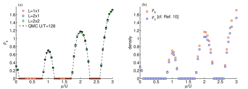
Figure 1: (Color online) Superfluid density $\rho_{s}$ (a) evaluated for constant hopping strength $t/U=0.02$ as a function of the chemical potential $\mu/U$. VCA results for reference systems of size $L=1\times 1$, $L=2\times 1$, and $L=2\times 2$ and for essentially infinitely large physical systems are compared to QMC results for physical systems of size $32\times 32$ and inverse temperature $U/T=128$. Comparison of the superfluid density $\rho_{s}$ and condensed density $\rho_{c}$ (b) for reference systems of size $L=1\times 1$ and essentially infinitely large physical systems, cf. Ref. Knap et al., 2011.

III Superfluid density

In this section we discuss the evaluation of the superfluid density $\rho_{s}$ within our extended SFA/VCA theory and present results for the two-dimensional BH model.

The superfluid density is related to the response of the system to a phase-twisting field,Fisher et al. (1973); Lieb et al. (2002) leading to twisted boundary conditions (BC) in one spatial direction, which we choose to be the ${\bf e}_{x}$-direction, and periodic BC in the others. The many-body wave function $\mathinner{|{\Psi}\rangle}$ has to obey these BC and thus

$$\hat{T}(N_{x}\,{\bf e}_{x})\mathinner{|{\Psi}\rangle}=e^{i\Theta}\mathinner{|{\Psi}\rangle}\;,$$

where the operator $\hat{T}({\bf r})$ translates the particles by the vector ${\bf r}$, $N_{x}$ is the lattice extension in ${\bf e}_{x}$-direction, and $\Theta$ is the phase twist applied to to the system. The twisted BC can be mapped by a unitary transformation onto the lattice Hamiltonian, leading to complex-valued hopping integrals.Roth and Burnett (2003); Rey et al. (2003); Poilblanc (1991) The resulting Hamiltonian can be interpreted as a cylinder rolled up along the $x$-direction, which is threaded by an effective magnetic field with total flux $\Theta$. When a particle is translated by $N_{x}$ in the ${\bf e}_{x}$-direction a phase $\exp[-i\Theta]$ is picked up.Scalapino et al. (1993) Due to gauge invariance, one is free to choose where the phase is collected when the particle propagates across the lattice. The usual choice is that each hopping process in the ${\bf e}_{x}$ direction, i. e., from site ${\bf r}^{\prime}=(r_{x}-1,\,r_{y})$ to ${\bf r}=(r_{x},\,r_{y})$, is multiplied by a phase factor $\exp[-iA]$, where the associated vector potential is

$$A=\Theta/N_{x}\;.$$ (31)

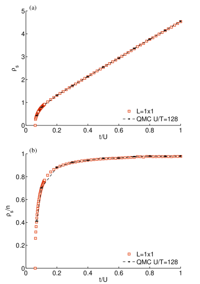
Figure 2: (Color online) Superfluid density $\rho_{s}$ (a) and superfluid fraction $\rho_{s}/n$ (b) ranging deep in the superfluid phase evaluated for constant chemical potential $\mu/U=0.4$ as a function of the hopping strength $t/U$. Results obtained by means of VCA for reference systems of size $L=1\times 1$ and essentially infinitely large physical systems are compared to QMC results for physical systems of size $32\times 32$ and inverse temperature $U/T=128$.

When choosing the phase in that way, the reference system $\hat{H}^{\prime}$ also depends on the vector potential $A$ and the intra-cluster hopping terms become complex-valued along the ${\bf e}_{x}$-direction. For a Hamiltonian with nearest-neighbor hopping $t$, the superfluid density is determined fromScalapino et al. (1993)

$$\rho_{s}=\frac{1}{t}\frac{1}{N_{x}\,N_{y}}\frac{\partial^{2}\,\Omega_{\Theta}}{\partial\,A^{2}}\;,$$ (32)

where $N_{x}\,N_{y}$ is the total number of lattice sites of the physical system, and $\Omega_{\Theta}$ is the grand potential of the physical system, subject to a phase twist $\Theta$, as discussed above. Plugging in the vector potential of Eq. (31) yields

$$\rho_{s}=\frac{1}{t}\frac{N_{x}}{N_{y}}\frac{\partial^{2}\,\Omega_{\Theta}}{\partial\,\Theta^{2}}\,.$$ (33)

In practice, the grand potential $\Omega_{\Theta}$ is evaluated at the stationary point of Eq. (30), and is determined self-consistently for several values of $\Theta$. From this data the curvature of $\Omega_{\Theta}$ with respect to $\Theta$ is extracted from a fit. Using the curvature, the superfluid density is evaluated according to Eq. (33). Note that a finite cluster is embedded in an essentially infinitely large system and thus the limits are taken in the correct order to obtain the superfluid density.Scalapino et al. (1993)

In the following, we apply this procedure to the two-dimensional BH modelFisher et al. (1989)

$$\hat{H}=\sum_{\left\langle i,\,j\right\rangle}t_{ij}\,a_{i}^{\dagger}\,a_{j}^{\phantom{\dagger}}+\frac{U}{2}\sum_{i}\hat{n}_{i}\left(\hat{n}_{i}-1\right)-\mu\sum_{i}\hat{n}_{i}\;\mbox{,}$$

where $a_{i}^{\dagger}$ ($a_{i}^{\phantom{\dagger}}$) creates (destroys) a bosonic particle on site $i$, and $\hat{n}_{i}=a_{i}^{\dagger}\,a_{i}^{\phantom{\dagger}}$ is the occupation number operator. The hopping integrals $t_{ij}$ are nonzero for nearest neighbors only, as indicated by the the angle brackets. Specifically, $t_{ij}=-t$ for hopping processes along the ${\bf e}_{y}$-direction and $t_{ij}=-t\exp[i\,A\,({\bf r}_{i}-{\bf r}_{j}){\bf e}_{x}]$ for hopping processes along the ${\bf e}_{x}$-direction. The chemical potential, termed $\mu$, controls the particle number and $U$ is the repulsive on-site interaction, which subsequently will be used as unit of energy. The reference system $\hat{H}^{\prime}$ consists of a cluster decomposition of the physical system $\hat{H}$ plus a $U(1)$ symmetry breaking source term

$$\hat{H}^{\prime}=\sum_{{\bf R}}\Big{[} \sum_{\left\langle\alpha,\,\beta\right\rangle}t^{\prime}_{\alpha\beta}a_{\alpha,{\bf R}}^{\dagger}\,a_{\beta,{\bf R}}^{\phantom{\dagger}}+\frac{U}{2}\sum_{\alpha}\hat{n}_{\alpha,{\bf R}}\left(\hat{n}_{\alpha,{\bf R}}-1\right)$$

$$-\mu^{\prime}\sum_{\alpha}\hat{n}_{\alpha,{\bf R}}-\sum_{\alpha}(a_{\alpha,{\bf R}}^{\dagger}\,f_{\alpha}^{\phantom{\dagger}}+f_{\alpha}^{*}\,a_{\alpha,{\bf R}}^{\phantom{\dagger}})\Big{]}\;\mbox{,}$$

where the lattice site indices $i$ have been decomposed into an index ${\bf R}$, that specifies the cluster and into an index $\alpha$, that specifies the lattice sites within a cluster.Knap et al. (2011, 2010) Analogously to the physical system, the hoping integrals are $t^{\prime}_{\alpha\beta}=-t^{\prime}$ and $t_{\alpha\beta}^{\prime}=-t^{\prime}\exp[i\,A\,({\bf r}_{{\bf R}\alpha}-{\bf r}_{{\bf R}\beta}){\bf e}_{x}]$ for nearest-neighbor hopping processes along the ${\bf e}_{y}$- and the ${\bf e}_{x}$-direction, respectively, and zero otherwise. In our calculation, we use the chemical potential $\mu^{\prime}$ and the source coupling strength $f_{\alpha}$ of the reference system as variational parameters in the optimization prescription. Since the reference system is complex valued, the source coupling strength $f_{\alpha}$ is complex valued too, i. e., $f_{\alpha}=|f_{\alpha}|\exp[\phi_{\alpha}]$. Thus, in general, $2L$ variational parameters have to be considered, where $L$ is the number of cluster sites. However, for different cluster sites $\alpha$ the source coupling strengths $f_{\alpha}$ are interrelated, as can be seen from mean field arguments, leading effectively to two variational parameters $|f|$ and $\phi$, which we use—in addition to the chemical potential $\mu^{\prime}$—to treat complex valued reference systems.

In Fig. 1 we present the superfluid density $\rho_{s}$ for different sizes of the reference system ranging from $L=1\times 1$, over $L=2\times 1$, to $L=2\times 2$ and essentially infinitely large physical systems. For the largest cluster we restrict the variational search space to real valued order parameters, i. e., we set $\phi_{\alpha}=0$. Figure 1 (a) demonstrates that this choice leads to comparable results as obtained with the full variational space. Yet, for the restricted variational space the computational effort as well as the numerical complexity is reduced, since the reference system remains real valued. Figure 1 (a) shows the superfluid density $\rho_{s}$, as a function of the chemical potential $\mu/U$ evaluated for fixed hopping strength $t/U=0.02$. The chemical potential ranges from $\mu/U=0$ to $\mu/U=3$. As the hopping strength is small, three regions with $\rho_{s}=0$ are present, corresponding to the Mott insulating phase. In between these regions, we observe a finite superfluid density $\rho_{s}$ indicating the occurrence of the superfluid phase. In addition to the VCA results, we show QMC results with errorbars (barely visible) for physical systems of size $32\times 32$ and inverse temperature $U/T=128$. The QMC calculations were performed with the ALPS libraryAlbuquerque et al. (2007) and the ALPS applications.Alet et al. (2005) Particularly, we use the stochastic series expansion representation of the partition function with directed loop updates,Sandvik and Kurkijärvi (1991); Evertz et al. (1993); Syljuåsen and Sandvik (2002) where the superfluid density is evaluated via the winding number.Pollock and Ceperley (1987); Prokof’ev and Svistunov (2000) The superfluid density $\rho_{s}$ obtained from VCA agrees remarkable well with the QMC results. Furthermore, VCA results are almost independent of the size $L$ of the reference system, signaling convergence to the correct results even for $L=1\times 1$ site clusters. The superfluid density $\rho_{s}$ is compared to the condensate density $\rho_{c}=\langle a_{i}\rangle$ in Fig. 1 (b), cf. Ref. Knap et al., 2011. It can be observed that the superfluid density is always larger than the density of the Bose-Einstein condensate. However, the difference between the two densities is rather small, since a very dilute Bose gas is investigated.

In Fig. 2 we evaluate (a) the superfluid density $\rho_{s}$ and (b) the superfluid fraction $\rho_{s}/n$ ($n$ is the particle density) for fixed chemical potential $\mu/U=0.4$ as a function of the hopping strength $t/U$. The hopping strength ranges from $t/U=0$ to $t/U=1$, which is already very deep in the superfluid phase. For $\mu/U=0.4$ the phase boundary between the Mott and the superfluid phase is located at $t/U\approx 0.06$. In the superfluid phase close to the phase boundary the superfluid density rises quickly from zero developing an almost linear behavior for $t/U\gtrsim 0.2$. In the latter parameter regime the superfluid fraction is larger than $90\%$ signaling that already a very large amount of the lattice bosons is superfluid. As emphasized in Ref. Rancon and Dupuis, 2010, a relatively sharp crossover from a strongly-correlated superfluid, characterized by a superfluid fraction which is well below $1$, to a weakly-correlated superfluid, where the superfluid fraction is almost $1$, can be observed, see Fig. 2 (b). In addition to the VCA results evaluated for reference systems of size $L=1\times 1$ and essentially infinitely large physical systems, we show QMC results for physical systems of size $32\times 32$ and inverse temperature $U/T=128$, which again exhibit perfect agreement.

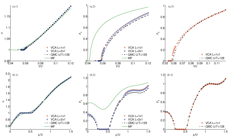
Figure 3: (Color online) Particle density $n$ (left), condensate density $\rho_{c}$ (middle), and superfluid density $\rho_{s}$ (right) evaluated around the quantum critical region close to the tip of the first Mott lobe. Comparison of the data obtained by means of VCA (for essentially infinitely large physical systems and reference systems as stated in the legends), QMC (for physical systems of size $32\times 32$ and inverse temperatures $U/T=128$), and mean-field. The first row (a.*) shows results for fixed chemical potential $\mu/U=0.4$ as a function of the hopping strength $t/U$, whereas the second row (b.*) shows results for fixed hopping strength $t/U=0.05$ as a function of the chemical potential $\mu/U$.

In Fig. 3 we focus on the quantum critical region close to the tip of the first Mott lobe, which is the most challenging one. In particular, we evaluate the particle density $n$, the condenstate density $\rho_{c}$, and superfluid density $\rho_{s}$. In the first row we show results for fixed chemical potential $\mu/U=0.4$ as a function of the hopping strength $t/U$, whereas in the second row we keep hopping strength fixed at $t/U=0.05$ and vary the chemical potential $\mu/U$. We compare VCA results with QMC and mean-field (MF). The most important observation is that MF is far off QMC and VCA. For $\mu/U=0.4$ MF predicts the phase transition to be at a much smaller value of $t/U$ than QMC and VCA. This leads to significant deviations in both the density and condensate density as compared to QMC and VCA. For fixed $t/U=0.05$ MF does not enter the Mott region and thus does not predict a plateau in the density. For both investigated situations (fixed $\mu/U$ and fixed $t/U$) the results obtained by means of VCA and QMC agree quite well. For the QMC simulations we used lattices of size $32\times 32$ and inverse temperatures of $U/T=128$. The VCA results are obtained at zero temperature for clusters of size $1\times 1$ and $2\times 1$, respectively, and essentially infinitely large physical systems. In this challenging regime small differences between VCA and QMC are observable for the condensate density. For the reference system sizes considered here, results are almost identical. Larger reference systems might still reduce the difference between VCA and QMC. However, close to the phase transition finite size and finite temperature effects might still be important for the QMC results, and thus a proper finite size scaling of these data might also reduce the discrepancy between the two approaches. Note that for fixed hopping $t/U=0.05$ there is a very small region at $\mu/U\approx 0.85$, where it is difficult to numerically determine the stationary point of the grand potential. Such a region is also present between the first and the second and between the second and the third Mott lobe in Fig. 1. However, there it is barely visible since the spacing between two consecutive $\mu$ datapoints is larger than this gap. This failure appears to be related to the fact that two solutions adiabatically connected to two sectors with different particle numbers, i. e. the two neighboring Mott regions, meet and try to avoid each other. However, we want to emphasize that this problem affects only a tiny region of the phase diagram. When keeping the chemical potential fixed at $\mu/U=0.4$ solutions can be easily found for all values of the hopping strength.

Finally, we want to emphasize that the VCA results are obtained with very modest computational effort and that excellent agreement with QMC can be observed, even for very small reference systems.

IV Conclusions

In the present work, we extend the self-energy functional approach to the $U(1)$ symmetry broken, superfluid phase of correlated lattice bosons. A crucial point of this extension is the identification of a quantity, termed $D$, which is the companion of the self-energy $\Sigma$ in the superfluid phase. We also identify the appropriate (nonuniversal) functional ${\hat{\Omega}}_{s}$ which is stationary at the physical values of the self-energy $\Sigma$ and of $D$. In analogy to the self-energy, which is the difference of the interacting and non-interacting Green’s function, the quantity $D$ is related to the difference of the order parameter of the interacting and non-interacting systems. Thus, $D$ is zero in the normal phase and for $U=0$. From these relations also follows that both $\Sigma$ as well as $D$ vanish in the non-interacting case. Importantly, when the functional ${\hat{\Omega}}_{s}$ is evaluated at the exact values of $\Sigma$ and $D$ it corresponds to the grand potential of the physical Hamiltonian. To evaluate the functional, we proceed as in the original self-energy functional approach,Potthoff (2003a) and introduce a reference system, which is a cluster decomposition of the physical system. Importantly, the reference system shares its two-particle interaction with the physical system, and can be exactly solved by numerical methods. By comparison of the functionals, the universal part of ${\hat{\Omega}}_{s}$, denoted as $\hat{\cal F}$, can be eliminated, which allows to evaluate ${\hat{\Omega}}_{s}$ exactly on the subspace of $\Sigma$ and $D$, spanned by the possible sets of reference systems. The results presented are shown to be equivalent to the ones obtained by a more heuristic method, the pseudoparticle approach introduced in Ref. Knap et al., 2011, and thus provide rigorous variational grounds for that approach. In addition, the extended self-energy functional approach introduced here allows to envision more general reference systems, in which bath sites are incorporated to enlarge the space of possible self-energies $\Sigma$, and possibly bridge over to (Cluster) Dynamical Mean Field Theory (DMFT).Potthoff (2003a); Georges et al. (1996) For future research it would be interesting to verify whether in the limit of an infinite number of bath sites and for a single correlated site as a reference system, our superfluid SFA becomes equivalent to DMFT for superfluid bosons,Byczuk and Vollhardt (2008); Anders et al. (2010) as it is the case in the normal phase.Potthoff (2003a) For a finite number of bath sites this is certainly not the case, since the order parameter in the reference system differs from the physical one.

We also presented how the superfluid density can be evaluated by means of this extended variational cluster approach. To this end we applied a phase twisting field to the system. We evaluated the superfluid density for the two-dimensional Bose-Hubbard model and compared the extended variational cluster approach results with unbiased quantum Monte Carlo results, yielding remarkable agreement. We want to emphasize that the extended self-energy functional approach is not only applicable to the Bose-Hubbard model but to a large class of lattice models, which exhibit a condensed phase. This includes experimentally interesting systems such as disordered bosons, multicomponent systems (Bose-Bose mixtures or Bose-Fermi mixtures) and light matter systems.Hartmann et al. (2008); Tomadin and Fazio (2010) Strictly speaking, the method cannot treat long-range interactions, such as dipolar ones, exactly.Barnett et al. (2006); Micheli et al. (2006) However, the long-range part can be incorporated on a mean-field level.Aichhorn et al. (2004) In principle, the present approach can be applied to systems with broken translational invariance as well, and, for example, can consider the effect of a confining magnetic trap. However, in this case one has to abandon the Fourier transform in the cluster vectors and work in real space and, thus, deal with larger matrices and a larger number of variational parameters. A convenient, numerically less expensive alternative, is to adopt the so-called local density approximation. Kollath et al. (2004)

Appendix A Notation and conventions

A.1 Matrix notation

A.1.1 General

In order to simplify our notation we omit time arguments, whenever this does not cause ambiguities. Therefore, two-point functions such as Green’s functions, self-energies, etc. are interpreted as matrices in Nambu, orbital, and $\tau$ space. One-point objects such as $\mathcal{A}$ ($\bar{\mathcal{A}}$) are interpreted as column (row) vectors in the same space. Matrix-matrix and vector-matrix products are understood throughout, whereby internal $\tau$ variables are considered to be integrated over. In addition, the transposing operator “^T” also acts on time variables. Traces $\operatorname{\mbox{Tr}}$ contain an integral over $\tau$ and a trace $\operatorname{\mbox{tr}}$ over orbital indices, i. e., $\operatorname{\mbox{Tr}}M\equiv\operatorname{\mbox{tr}}\int_{0}^{\beta}d\tau M(\tau,\tau+0^{+})$, where the $0^{+}$ leads to the well known convergence factor $e^{i\omega_{n}0^{+}}$ in Matsubara space.

(Functional) derivatives with respect to matrices are defined “transposed”:

$$\left(\frac{\delta\hat{X}}{\delta M}\right)_{ij}(\tau,\tau^{\prime})\equiv\frac{\delta\hat{X}}{\delta M_{ji}(\tau^{\prime},\tau)}\;.$$

Finally, there are two types of products between row (in the form $\bar{v}$) and column ($u$) vectors, depending on the order: On the one hand the product $\bar{v}u$ produces a scalar (all indices are summed/integrated over). On the other hand, inverting the order, as in $u\bar{v}$ gives a matrix, as indices are “external” and, thus, not summed over.

A.1.2 Trace in $\tau$ and in Matsubara space

In $\tau$ space we have

$$\operatorname{\mbox{Tr}}M=\beta^{-1}{\operatorname{\mbox{tr}}}\int_{0}^{\beta}d\tau\ M(\tau,\tau+0^{+})\;.$$

The transformation of $M(\tau,\tau^{\prime})$ to Matsubara space is defined as

$$M(\tau,\tau^{\prime})\equiv\beta^{-1}\sum_{n,n^{\prime}}M(\omega_{n},\omega_{n}^{\prime})e^{-i\omega_{n}\tau+i\omega_{n}^{\prime}\tau^{\prime}}\;.$$

The inverse transformation reads

$$M(\omega_{n},\omega_{n}^{\prime})=\beta^{-1}\int d\tau d\tau^{\prime}M(\tau,\tau^{\prime})e^{i\omega_{n}\tau-i\omega_{n}^{\prime}\tau^{\prime}}\;.$$

Combining the equations above, the trace becomes

$$\operatorname{\mbox{Tr}}M ={\operatorname{\mbox{tr}}}\int_{0}^{\beta}d\tau\beta^{-2}\sum_{n,n^{\prime}}M(\omega_{n},\omega_{n}^{\prime})e^{-i(\omega_{n}-\omega_{n}^{\prime})\tau+i\omega_{n}^{\prime}0^{+}}$$

$$=\beta^{-1}\sum_{n}{\operatorname{\mbox{tr}}}M(\omega_{n},\omega_{n})e^{i\omega_{n}0^{+}}\;.$$

A.1.3 Logarithm

There are some subtle points concerning logarithms of two-point functions. Although these issues are immaterial for the final result, we prefer to specify them in detail.

The logarithm of $G$ considered as a matrix in the continuum variable $\tau$ is defined up to an infinite constant which depends on the the discretization step $\delta$ (see below). In addition, the trace of the logarithm carried out in Matsubara space diverges as well (despite the convergence factor $e^{i\omega_{n}0^{+}}$). The usual result presented in the literature (see, for instance Ref. Luttinger and Ward, 1960) implicitly assumes that an infinite constant has been subtracted. In order to avoid these undetermined infinite terms, we subtract them explicitly at the outset with the help of the “infinite energy” Green’s function

$$G_{\infty}(\tau,\tau^{\prime}) =\beta^{-1}\sum_{n}G_{\infty}(\omega_{n})e^{-i\omega_{n}(\tau-\tau^{\prime})}$$

$$G_{\infty}(\omega_{n}) =\mathbbm{1}\frac{1}{i\omega_{n}-E}\;,$$

where it is understood that the $E\to+\infty$ limit is taken at the end of the calculation. This choice guarantees, for example, that $\operatorname{\mbox{Tr}}\ln G/G_{\infty}$, where $G$ is the Green’s function in normal (i.e. not Nambu) notation, vanishes in the limit $\mu\to-\infty$, where $\mu$ is the chemical potential.

The Fourier transform defined in App. A.1.2 allows to define the logarithm of $G$ in $\tau$ space, apart from an infinite multiplicative constant, which originates from the fact that the Fourier transformation is not and cannot be normalized in the continuum limit. In particular,

$$[\ln(-G)](\tau,\tau^{\prime}) =\beta^{-1}\sum_{n,n^{\prime}}[\ln(-G)](\omega_{n},\omega_{n}^{\prime})e^{-i\omega_{n}\tau+i\omega_{n}^{\prime}\tau^{\prime}}$$

$$=\beta^{-1}\sum_{n}\ln\left[-G(\omega_{n})\right]e^{-i\omega_{n}(\tau-\tau^{\prime})}\;,$$

A.2 Symmetry of Green’s functions and other two-point functions

The action in Eq. (5) is invariant under the transformation $G_{0}\to({\cal T}G_{0}^{T}{\cal T})$, where the transposing operator “^T” also acts on time variables and ${\cal T}$ is defined in Eq. (8). This is due to the fact that

$$\bar{A}(\tau^{\prime})G_{0}^{-1}(\tau^{\prime},\tau)A(\tau)=A(\tau^{\prime})^{T}{\cal T}G_{0}^{-1}(\tau^{\prime},\tau){\cal T}\bar{A}(\tau)^{T}\\ =\bar{A}(\tau)({\cal T}G_{0}^{-1}(\tau^{\prime},\tau)^{T}{\cal T})A(\tau^{\prime})\;.$$

Therefore, we choose $G_{0}$ to obey the symmetry

$$G_{0}=({\cal T}G_{0}^{T}{\cal T})\;.$$ (34)

The same symmetry is obeyed by other two-point functions, such as the interacting Green’s function $G$, the self-energy $\Sigma$, and their inverse.

In principle, this redundancy renders relations such as Eq. (15) non invertible. In order to avoid this, we adopt the convention that functional inversions are carried out within the subspace of two-point functions obeying the relation Eq. (34). In addition, we adopt the following convention for functional derivatives of an arbitrary functional $\hat{\Xi}$ with respect to a two-point function $X$:

$$\frac{\delta\hat{\Xi}}{\delta X}\to\frac{1}{2}\left(\frac{\delta\hat{\Xi}}{\delta X}+\frac{\delta\hat{\Xi}}{\delta{\cal T}X^{T}{\cal T}}\right)\;.$$

A.3 Continuum limit of the functional integral

In principle, the expression Eq. (10) should be understood such that adjoint fields $\bar{a}$ are evaluated at a later imaginary time $\tau+\delta$, whereby $\delta$ is the width of the discretization mesh of the interval $(0,\beta)$. The continuum limit $\delta\to 0$ should be taken after having carried out the functional integration, see, e.g. Ref. Schulman, 1981. Taking this limit at the outset amounts to neglecting the so-called “contribution from infinity”. Arrigoni et al. (1994); Arrigoni and Strinati (1993) This can be achieved by effectively replacing the normal-ordered Hamiltonian with a “symmetrically ordered” one, which is suitably symmetrized among possible permutation of creation and annihilation operators. Arrigoni and Strinati (1995) In particular, for the noninteracting part, this amounts to replacing the operator expression $a^{\dagger}a$ by $\frac{1}{2}(a^{\dagger}a+aa^{\dagger})=a^{\dagger}a+\frac{1}{2}$. Therefore, we should keep in mind that the grand-potential ${\widetilde{\Omega}}_{s}$ corresponds to such a symmetrized Hamiltonian.

References

- Jaksch et al. (1998) D. Jaksch, C. Bruder, J. I. Cirac, C. W. Gardiner, and P. Zoller, Phys. Rev. Lett. 81, 3108 (1998).
- Greiner et al. (2002) M. Greiner, O. Mandel, T. Esslinger, T. W. Hansch, and I. Bloch, Nature 415, 39 (2002).
- Bloch et al. (2008) I. Bloch, J. Dalibard, and W. Zwerger, Rev. Mod. Phys. 80, 885 (2008).
- Gerbier et al. (2008) F. Gerbier, S. Trotzky, S. F???lling, U. Schnorrberger, J. D. Thompson, A. Widera, I. Bloch, L. Pollet, M. Troyer, B. Capogrosso-Sansone, et al., Phys. Rev. Lett. 101, 155303 (2008).
- Trotzky et al. (2010) S. Trotzky, L. Pollet, F. Gerbier, U. Schnorrberger, I. Bloch, N. V. Prokof’ev, B. Svistunov, and M. Troyer, Nat. Phys. 6, 998 (2010), ISSN 1745-2473.
- Kato et al. (2008) Y. Kato, Q. Zhou, N. Kawashima, and N. Trivedi, Nat Phys 4, 617 (2008), ISSN 1745-2473.
- Diener et al. (2007) R. B. Diener, Q. Zhou, H. Zhai, and T. L. Ho, Phys. Rev. Lett. 98, 180404 (2007).
- Roth and Burnett (2003) R. Roth and K. Burnett, Phys. Rev. A 67, 031602 (2003).
- Cooper and Hadzibabic (2010) N. R. Cooper and Z. Hadzibabic, Phys. Rev. Lett. 104, 030401 (2010).
- Knap et al. (2011) M. Knap, E. Arrigoni, and W. von der Linden, Phys. Rev. B 83, 134507 (2011).
- Koller and Dupuis (2006) W. Koller and N. Dupuis, J. Phys.: Condens. Matter 18, 9525 (2006).
- Potthoff (2003a) M. Potthoff, Eur. Phys. J. B 32, 429 (2003a).
- Potthoff (2003b) M. Potthoff, Eur. Phys. J. B 36, 335 (2003b).
- Zacher et al. (2002) M. G. Zacher, R. Eder, E. Arrigoni, and W. Hanke, Phys. Rev. B 65, 045109 (2002).
- Fisher et al. (1973) M. E. Fisher, M. N. Barber, and D. Jasnow, Phys. Rev. A 8, 1111 (1973).
- Pollock and Ceperley (1987) E. L. Pollock and D. M. Ceperley, Phys. Rev. B 36, 8343 (1987).
- Prokof’ev and Svistunov (2000) N. V. Prokof’ev and B. V. Svistunov, Phys. Rev. B 61, 11282 (2000).
- Fisher et al. (1989) M. P. A. Fisher, P. B. Weichman, G. Grinstein, and D. S. Fisher, Phys. Rev. B 40, 546 (1989).
- (19) See App. A.2.
- Potthoff (2006) M. Potthoff, Condens. Matt. Phys. 9, 557 (2006).
- (21) Here, and below we assume that the relations between conjugate variables are invertible, at least locally, see also App. A.2.
- Potthoff et al. (2003) M. Potthoff, M. Aichhorn, and C. Dahnken, Phys. Rev. Lett. 91, 206402 (2003).
- (23) In VCA Potthoff (2003a); Dahnken et al. (2004) the reference system is typically a cluster partition of the original lattice, which can be improved by including bath sites. Balzer et al. (2008, 2009) However, for bosonic systems with and the Hilbert space is infinite and the particle number is not conserved. Thus neither a cluster nor a single site can be solved by exact diagonalization. However, a cutoff in the maximum number of bosons can be introduced, which still allows to reach arbitrary accuracy.
- (24) The term with (see App. A.3) cancels out.
- Balzer et al. (2008) M. Balzer, W. Hanke, and M. Potthoff, Phys. Rev. B 77, 045133 (2008).
- Balzer et al. (2009) M. Balzer, W. Hanke, and M. Potthoff (2009), arXiv:0912.1282.
- Lieb et al. (2002) E. H. Lieb, R. Seiringer, and J. Yngvason, Phys. Rev. B 66, 134529 (2002).
- Rey et al. (2003) A. M. Rey, K. Burnett, R. Roth, M. Edwards, C. J. Williams, and C. W. Clark, J. Phys. B 36, 825 (2003).
- Poilblanc (1991) D. Poilblanc, Phys. Rev. B 44, 9562 (1991).
- Scalapino et al. (1993) D. J. Scalapino, S. R. White, and S. Zhang, Phys. Rev. B 47, 7995 (1993).
- Knap et al. (2010) M. Knap, E. Arrigoni, and W. von der Linden, Phys. Rev. B 81, 024301 (2010).
- Albuquerque et al. (2007) A. Albuquerque, F. Alet, P. Corboz, P. Dayal, A. Feiguin, S. Fuchs, L. Gamper, E. Gull, S. Gürtler, A. Honecker, et al., J. Magn. Magn. Mater. 310, 1187 (2007).
- Alet et al. (2005) F. Alet, S. Wessel, and M. Troyer, Phys. Rev. E 71, 036706 (pages 16) (2005).
- Sandvik and Kurkijärvi (1991) A. W. Sandvik and J. Kurkijärvi, Phys. Rev. B 43, 5950 (1991).
- Evertz et al. (1993) H. G. Evertz, G. Lana, and M. Marcu, Phys. Rev. Lett. 70, 875 (1993).
- Syljuåsen and Sandvik (2002) O. F. Syljuåsen and A. W. Sandvik, Phys. Rev. E 66, 046701 (2002).
- Rancon and Dupuis (2010) A. Rancon and N. Dupuis, arXiv:1012.0166 (2010).
- Georges et al. (1996) A. Georges, G. Kotliar, W. Krauth, and M. J. Rozenberg, Rev. Mod. Phys. 68, 13 (1996).
- Byczuk and Vollhardt (2008) K. Byczuk and D. Vollhardt, Phys. Rev. B 77, 235106 (2008).
- Anders et al. (2010) P. Anders, E. Gull, L. Pollet, M. Troyer, and P. Werner, Phys. Rev. Lett. 105, 096402 (2010).
- Hartmann et al. (2008) M. Hartmann, F. G. Brandão, and M. B. Plenio, Laser & Photonics Review 2, 527 (2008).
- Tomadin and Fazio (2010) A. Tomadin and R. Fazio, J. Opt. Soc. Am. B 27, A130 (2010).
- Barnett et al. (2006) R. Barnett, D. Petrov, M. Lukin, and E. Demler, Phys. Rev. Lett. 96, 190401 (2006).
- Micheli et al. (2006) A. Micheli, G. K. Brennen, and P. Zoller, Nat. Phys. 2, 341 (2006), ISSN 1745-2473.
- Aichhorn et al. (2004) M. Aichhorn, H. G. Evertz, W. von der Linden, and M. Potthoff, Phys. Rev. B 70, 235107 (2004).
- Kollath et al. (2004) C. Kollath, U. Schollwöck, J. von Delft, and W. Zwerger, Phys. Rev. A 69, 031601 (2004).
- Luttinger and Ward (1960) J. M. Luttinger and J. C. Ward, Phys. Rev. 118, 1417 (1960).
- Schulman (1981) L. S. Schulman, Techniques and Applications of Path Integration (Wiley, New York, 1981).
- Arrigoni et al. (1994) E. Arrigoni, C. Castellani, M. Grilli, R. Raimondi, and G. C. Strinati, Phys. Rep. 241, 291 (1994).
- Arrigoni and Strinati (1993) E. Arrigoni and G. C. Strinati, Phys. Rev. Lett. 71, 3178 (1993).
- Arrigoni and Strinati (1995) E. Arrigoni and G. C. Strinati, Phys. Rev. B 52, 2428 (1995).
- Dahnken et al. (2004) C. Dahnken, M. Aichhorn, W. Hanke, E. Arrigoni, and M. Potthoff, Phys. Rev. B 70, 245110 (2004).