A closed contact cycle on the ideal trefoil

Abstract

Numerical computations suggest that each point on a certain optimized shape called the ideal trefoil is in contact with two other points. We consider sequences of such contact points, such that each point is in contact with its predecessor and call it a billiard. Our numerics suggest that a particular billiard on the ideal trefoil closes to a periodic cycle after nine steps. This cycle also seems to be an attractor: all billiards converge to it.

Institut de Mathématiques B, École Polytechnique Fédérale de Lausanne, CH-1015 Lausanne, Switzerland, {mathias.carlen, henryk.gerlach}@gmail.com

1 Introduction

A closed curve in $\mathbb{R}^{3}$ is called ideal if it minimizes its ropelength $\mathcal{L}[\cdot]/\Delta[\cdot]$ – i.e. its length divided by its thickness – within its knot class [12]. In this paper we will focus on the simplest of all proper ideal knots, namely the trefoil knot. Various numerical approximations of this specific knot are available. It is not trivial to define what the properties of a “good” approximation are. Quantities like ropelength, functions such as curvature and torsion, or the contact set for a given knot are can all be used to assess whether a knot is close to ideal. There exist several algorithms to compute ideal knot shapes, which use different approximations for the curve description[16, 10, 20, 7, 1]. These numerical computations are expected to lead to a better understanding of ideal knots. In this sense a numerical shape is “good”, if it leads to more insight about properties of ideal knots.

A curve is in contact with itself at the points $p,q$ if the distance between $p$ and $q$ is precisely two times the thickness of the curve and the line segment between them is orthogonal to the curve at both ends. [21, 10] define a robust sense of contact with a tolerance and their computations suggest that each point on the ideal trefoil in $\mathbb{R}^{3}$ is in contact with two other points . Starting from a point $p_{0}$, it is in contact with a point $p_{1}$ that itself is again in contact with a point $p_{2}\neq p_{0}$ and so on. Does this sequence close to a cycle? In this article we observe that computations suggest that the ideal trefoil knot has a periodic, and attracting nine-cycle of contact chords, as illustrated in Figure 1.

A similar construction of periodic cycles, but in each point of the curve, helped to construct the ideal Borromean rings [22, 5]. The existence of this cycle is significant because it partitions the trefoil in such a way that, using the apparent symmetries, it can be re-constructed from two unknown small pieces of curves mutually in contact.

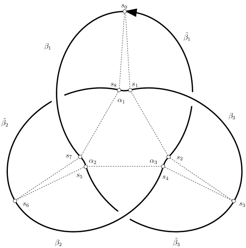
Figure 1: The parameters $s_{i}:=\sigma^{i}(0)$ of the nine-cycle $b_{9}$ partition the trefoil in 9 curves: $\beta_{i}$ and $\tilde{\beta_{i}}$ are all congruent as are $\alpha_{i}$ ($i=1,2,3$). The contact function $\sigma$ maps the parameter interval of each curve bijectively to the parameter interval of another curve (see Figure 6).

We approximated the ideal trefoil using a Fourier representation described in [9]. The numerical computations were carried out with libbiarc [17] and the data is available from [14]. The numerical Fourier trefoil is not the best known in ropelength sense, but – to our knowledge – the best shape to observe the closed cycle, probably because we can enforce specific symmetries.

Another interesting discovery is that, if we follow the contact chords starting at an arbitrary point on the trefoil, we always end up at the previously mentioned cycle, in other words, it is a global attractor.

In order to present this closed cycle on the trefoil we first review the notions of global radius of curvature [12] and contact of a curve [19, 10] in Section 2. Section 3 introduces contact billiards and cycles. Then we present and discuss a candidate for a cycle in the trefoil and show numerically that it seems to act as an attractor for all the billiards on the trefoil.

2 The Ideal Trefoil – Its Contact Chords and Symmetries

A knot is a closed curve $\gamma\in C^{1}(\mathbb{S},\mathbb{R}^{3})$ where $\mathbb{S}:=\mathbb{R}/\mathbb{Z}$ is the unit interval with the endpoints identified, isomorphic to the unit circle. We use the global radius of curvature to assign a thickness $\Delta$ to $\gamma$.

Definition 1 (Global radius of curvature).

[12] For a $C^{0}$-curve $\gamma:\mathbb{S}\longrightarrow\mathbb{R}^{3}$ the global radius of curvature at $s\in\mathbb{S}$ is

$$\rho_{G}[\gamma](s):=\inf_{\sigma,\tau\in\mathbb{S},\sigma\not=\tau,\sigma\not=s,\tau\not=s}R(\gamma(s),\gamma(\sigma),\gamma(\tau)).$$ (1)

Here $R(x,y,z)\geq 0$ is the radius of the smallest circle through the points $x,y,z\in\mathbb{R}^{3}$, i.e.

$$R(x,y,z):=\left\{\begin{array}[]{cl}\frac{|x-z|}{2\sin\measuredangle(x-y,y-z)}&\mbox{$x,y,z$ not collinear},\\ \infty&\mbox{$x,y,z$ collinear, pairwise distinct},\\ \frac{{\rm diam}(\{x,y,z\})}{2}&\mbox{otherwise}.\end{array}\right.$$

where $\measuredangle(x-y,y-z)\in[0,\pi/2]$ is the smaller angle between the vectors $(x-y)$ and $(y-z)\in\mathbb{R}^{3}$, and

$${\rm diam}(M):=\sup_{x,y\in M}|x-y|\;\mbox{for}\;M\subset\mathbb{R}^{3}$$

is the diameter of the set $M$. The thickness of $\gamma$, denoted as

$$\Delta[\gamma]:=\inf_{s\in\mathbb{S}}\rho_{G}[\gamma](s)=\inf_{s,\sigma,\tau\in\mathbb{S},\sigma\not=\tau,\sigma\not=s,\tau\not=s}R(\gamma(s),\gamma(\sigma),\gamma(\tau)),$$ (2)

is defined as the infimum of $\rho_{G}$.

A curve that minimizes arclength over thickness is called an ideal knot [15, 12]. Already [12] showed in a $C^{2}$-setting that for a knot to be ideal, $\rho_{G}$ around a parameter is either constant and equal to the infimum, or the curve is locally a straight line. A proof of this necessary condition for $C^{1,1}$ curves is not known yet. Assume for a moment, that $\gamma$ is ideal and $C^{2}$, then for each $t\in\mathbb{S}$ we distinguish the following three cases [12, 18]:

1. $\rho_{G}(t)>\Delta[\gamma]$ and there exists $\varepsilon>0$ such that $\gamma(\{s:|s-t|<\varepsilon\})$ is a straight line.

2. $\rho_{G}(t)=\Delta[\gamma]$ and the curvature of $\gamma$ at $t$ is $1/\Delta[\gamma]$.

3. $\rho_{G}(t)=\Delta[\gamma]$ and there exists a $s\in\mathbb{S}$ with $|\gamma(s)-\gamma(t)|=2\Delta[\gamma]$ and $\langle\gamma^{\prime}(s),\gamma(s)-\gamma(t)\rangle=\langle\gamma^{\prime}(t),\gamma(s)-\gamma(t)\rangle=0$.

In case (B) we say that global curvature is attained locally, or that curvature is active, while in case (C) we say that the contact is global. The global contact is realized by a contact chord.

Definition 2 (Contact Chord).

Let $\gamma\in C^{1}(\mathbb{S},\mathbb{R}^{3})$ be a regular, i.e. $|\gamma^{\prime}(s)|>0$, curve with $\Delta[\gamma]>0$ and let $s,t\in\mathbb{S}$ be such that $c(s,t):=\gamma(t)-\gamma(s)$ has length

$$|c(s,t)|=2\Delta[\gamma],$$

and $c(s,t)$ is orthogonal to $\gamma$, i.e. $\langle\gamma^{\prime}(s),c(s,t))\rangle=\langle\gamma^{\prime}(t),c(s,t)\rangle=0,$ then we call $c(s,t)$ a contact chord. If such $s$ and $t$ exist, we say $\gamma$ has a contact chord connecting $\gamma(s)$ and $\gamma(t)$ or the parameters $s$ and $t$ are (globally) in contact. The set

$$\{\gamma(s)+hc(s,t):h\in[0,1]\}\subset\mathbb{R}^{3}$$

will also be called a contact chord. Being in contact is a symmetric relation.

Name	k3_1
Degrees of freedom	165
Biarc nodes	333
Arclength $\mathcal{L}$	1
Thickness $\Delta$	0.030539753
Ropelength $\mathcal{L}/\Delta$	32.744208

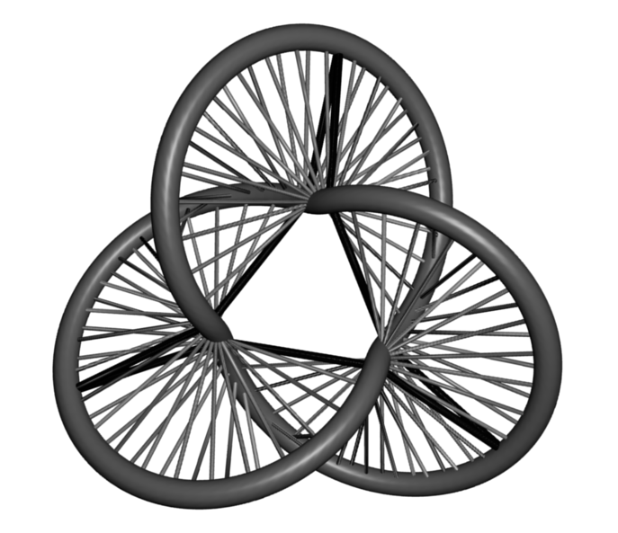
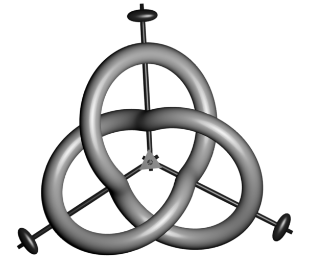
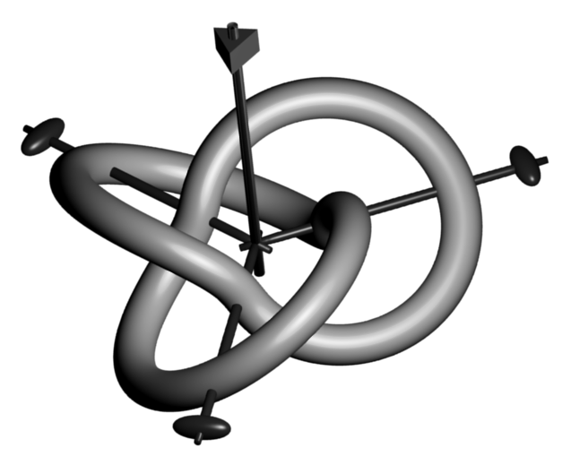
(a)	(b)	(c)

Figure 2: In the top box we describe the data for the trefoil used for the computations. In the bottom row we have (a) the trefoil with a few contact chords. The dark chords visualize the closed cycle in the contact chords of the trefoil. The pictures (b) and (c) illustrate two different views of plausible symmetry axes. The $120^{\circ}$ rotation axis and the three $180^{\circ}$ rotation axes are decorated with a prism and an ellipsoid at the end, respectively.

For the rest of the article, we will restrict ourselves to the ideal trefoil $\gamma_{3_{1}}$. The trefoil data used in this article was computed as in [9]. A Fourier representation of the knot makes enforcing symmetries natural. The specific symmetries are proposed in Conjecture 1. They significantly reduce the number of independent Fourier parameters in simulated annealing [16], while the computation of the thickness is done by interpolating the Fourier knot with biarcs [10, 9]. The Fourier coefficients and the point-tangent data for the trefoil are available online (see also Figure 2).

The numeric approximations of the ideal trefoil suggest that every point is globally in contact with two other points on the trefoil [10]. We can sort the contact chords in a continuous fashion, such that each point has an incoming and an outgoing contact. In our numerical computations of the contact chords we used the point-to-point distance function

$${\rm pp}(s,\sigma):=|\gamma(s)-\gamma(\sigma)|.$$

The general belief is that the ${\rm pp}$-function of the ideal trefoil has an extremely flat double valley away from the diagonal [10] (see Figure 3 for a 3D version of ${\rm pp}(s,\sigma)$ for the trefoil). For a sampling $s_{i}:=i/n$, $i=0,\ldots,n$, we compute $\sigma_{i}$ as the minimum of ${\rm pp}(s_{i},\cdot)$ restricted to the region $[\sigma_{i-1}-\varepsilon,\sigma_{i-1}+\varepsilon]$, $1\gg\varepsilon>0$. The initial value $(s_{0},\sigma_{0})$ is computed as the local minimum away from the diagonal. We now choose one of the two valley floors. By staying close to the previously computed minimum, we never cross over to the second valley. We then linearly interpolate between the $(s_{i},\sigma_{i})$ pairs to obtain an approximation of the so called contact function $\sigma$ (also see Figure 6 below for a top view of $\sigma$):

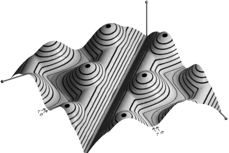
Figure 3: The distance function ${\rm pp}(s,\sigma)$ for $s,\sigma\in\mathbb{S}$ goes to $0$ on the diagonal and forms a large valley with two very shallow sub-valleys. The dotted lines marked with arrows in the valley indicate the two local minima, i.e. $\sigma(s)$ and $\tau(s)$.

Definition 3 (Contact functions).

Let $\sigma:\mathbb{S}\longrightarrow\mathbb{S}$ be a continuous, bijective and orientation preserving function, such that $\gamma_{3_{1}}(s)-\gamma_{3_{1}}(\sigma(s))$ is a contact chord for every $s\in\mathbb{S}$. The inverse function of $\sigma$ is $\tau:=\sigma^{-1}$.

As mentioned previously, numerics point out that the trefoil is symmetric with respect to a specific symmetry group [10, 3, 9]. These symmetries have helped to identify the closed cycle proposed later in this article.

Conjecture 1 (Symmetry of the ideal trefoil).

The ideal trefoil has symmetries as shown in Figure 2.

The symmetries of the trefoil are also apparent in its contact functions $\sigma$ and $\tau$. The relations are listed in the following lemma.

Lemma 1 (Symmetry of $\sigma,\tau$).

Assume Conjecture 1 about the symmetry of the constant speed parameterized trefoil $\gamma_{3_{1}}:\mathbb{S}\longrightarrow\mathbb{R}^{3}$ is true. Then the contact functions $\sigma,\tau:\mathbb{S}\longrightarrow\mathbb{S}$ have the following properties:

$$\sigma(s^{*}+t) \stackrel{{\scriptstyle\text{in\;}\mathbb{S}}}{{=}} -\tau(s^{*}-t),\quad\forall t\in\mathbb{S}$$ (3)

$$\sigma(t+1/3) \stackrel{{\scriptstyle\text{in\;}\mathbb{S}}}{{=}} \sigma(t)+1/3,\quad\forall t\in\mathbb{S}$$ (4)

$$\tau(s^{*}+t) \stackrel{{\scriptstyle\text{in\;}\mathbb{S}}}{{=}} -\sigma(s^{*}-t),\quad\forall t\in\mathbb{S}$$ (5)

$$\tau(t+1/3) \stackrel{{\scriptstyle\text{in\;}\mathbb{S}}}{{=}} \tau(t)+1/3,\quad\forall t\in\mathbb{S}$$ (6)

where $s^{*}\in\mathbb{S}$ is a parameter such that $\gamma_{3_{1}}(s^{*})$ is on a $180^{\circ}$ rotation axis. ∎

3 Closed Cycles

Recall from the previous section that numerics suggest that every point on the ideal trefoil $\gamma_{3_{1}}$ is in contact with two other points and we assume to be able to define a contact function $\sigma$ as in Definition 3. Is there a finite tuple of points such that each parameter is in contact with, and only with, its cyclic predecessor and successor? Inspired by Dynamical Systems [4] we call a sequence of parameters that are in contact with each predecessor a billiard. If a billiard closes, we call it a cycle:

Definition 4 (Cycle).

For $n\in\mathbb{N}$ let $b:=(t_{0},\ldots,t_{n-1})\in\mathbb{S}\times\cdots\times\mathbb{S}$ be an $n$-tuple. We call $b$ an $n$-cycle if $\sigma(t_{i})=t_{i+1}$ for $i=0,\ldots,n-2$ and $\sigma(t_{n-1})=t_{0}$, where $\sigma$ is defined as in Definition 3. The cycle $b$ is called minimal if all $t_{i}$ are pairwise distinct.

Each cyclic permutation of a cycle is again a cycle. Basing the definition of cycles on the continuous function $\sigma$ instead of closed polygons in $\mathbb{R}^{3}$ makes it slightly easier to find them numerically:

Remark 1.

The $\gamma_{3_{1}}$ has an $n$-cycle iff there exists some $t\in\mathbb{S}$ such that

$$\sigma^{n}(t):=\underbrace{\sigma\circ\cdots\circ\sigma}_{n\text{ times }}(t)=t.$$

The cycle is then $b:=(t,\sigma^{1}(t),\ldots,\sigma^{n-1}(t))$. $\Box$

All parameters of a minimal $n$-cycle are pairwise distinct so each minimal $n$-cycle corresponds to $n$ points in the set $\{t\in\mathbb{S}:\sigma^{n}(t)=t\}$. Since there are $n$ cyclic permutations of an $n$-cycle and since minimal $n$-cycles that are not cyclic permutations must be point-wise distinct this leads to:

Lemma 2 (Counting Cycles).

Define the set of intersections of $\sigma^{n}$ with the diagonal $I:=\{t\in\mathbb{S}:\sigma^{n}(t)=t\}$. If there is a finite number of minimal $n$-cycles then

$$\#I \geq (\text{Number of distinct minimal $n$-cycles})\cdot n$$

$$= (\text{Number of minimal $n$-cycles}).$$

∎

In Figure 4 we compiled small plots of $\sigma^{n}$ for $n=1,\ldots,27,144$. For $n=2$ the function $\sigma^{2}$ comes close to the diagonal for the first time, but can not touch it in less than three points by Lemma 1. If it would touch it would have to touch at least six times by Lemma 2, which does not seem to be the case.

By similar arguments, we exclude the possibility of cycles for $n=7,$ $11,$ $13,$ $16,$ $20$ and $25$. On the other hand the case $n=9$ looks promising (see Figure 5). It seems to touch the diagonal precisely nine times which suggests the existence of a single minimal cycle $b_{9}$ and its cyclic permutations. With our parameterization the cycle $b_{9}$ happens to start at $0$ and we compute a numerical error of only $\sigma^{9}(0)=0.0007\approx 0$. Consequently the cases $n=18,27$ would also touch the diagonal, but the corresponding cycle would not be minimal. We studied the plots till $n=100$, but did not find any other promising candidates (apart from $n=k\cdot 9$ for $k\in\mathbb{N}$). Keep in mind that the numerical error increases with $n$, but even for $n=144$ the graph looks reasonable.

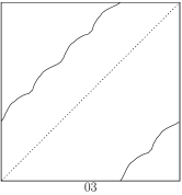
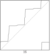
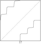
Figure 4: Plots of $\sigma^{n}:\mathbb{S}\longrightarrow\mathbb{S}$. In plot 09 the function $\sigma^{9}$ seems to touch the diagonal (see also Figure 5 for an enlarged plot). Accordingly $\sigma^{i}$ touches the diagonal in plot $i$ for $i\in\{9,18,27,\dots\}$. Note that in plot 144 the numerical errors have added up so that $\sigma^{144}$ no longer touches the diagonal.

We believe that $b_{9}$ is indeed a cycle (see Figure 1):

Conjecture 2 (Existence of nine-cycle).

Let $\gamma_{3_{1}}:\mathbb{S}\longrightarrow\mathbb{R}^{3}$ be the ideal trefoil, parameterized with constant speed such that $\gamma_{3_{1}}(0)$ is the outer point of the trefoil on a symmetry axis. Then $b_{9}=(s_{0},\ldots,s_{8})$ with $s_{i}:=\sigma^{i}(0)$ is a nine-cycle. Numerics suggest that $\gamma_{3_{1}}$ passes from 0 to 1 through $s_{i}$ in the sequence: $s_{0},s_{7},s_{5},s_{3},s_{1},s_{8},s_{6},s_{4},s_{2}$.

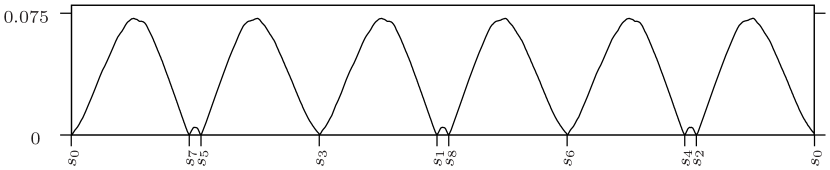
Figure 5: The plot shows graph number $9$ from Figure 4 rotated by $45^{\circ}$. It seems to touch the diagonal 9 times in the points $s_{0}=0$, $s_{7}=0.159$, $s_{5}=0.175$, $s_{3}=0.334\approx 1/3$, $s_{1}=0.492$, $s_{8}=0.508$, $s_{6}=0.667\approx 2/3$, $s_{4}=0.826$, $s_{2}=0.841$. This indicates the existence of a nine-cycle $b_{9}=(0,\sigma^{1}(0),\ldots,\sigma^{8}(0))$.

Note that $b_{9}$ partitions the trefoil in 9 parts (see Figure 1): Three curves

$$\beta_{1} := \gamma_{3_{1}}|_{[s_{0},s_{7}]},$$

$$\beta_{2} := \gamma_{3_{1}}|_{[s_{6},s_{4}]},$$

$$\beta_{3} := \gamma_{3_{1}}|_{[s_{3},s_{1}]},$$

$$\text{or}\;\beta_{i} := \gamma_{3_{1}}|_{[s_{6(i-1)},s_{6(i-1)-2}]}\;\text{with}\;s_{k}=s_{k+9},$$

which are congruent by $120^{\circ}$ rotations around the $z$-axis. Another three curves

$$\tilde{\beta_{1}} := \gamma_{3_{1}}|_{[s_{2},s_{0}]},$$

$$\tilde{\beta_{2}} := \gamma_{3_{1}}|_{[s_{8},s_{6}]},$$

$$\tilde{\beta_{3}} := \gamma_{3_{1}}|_{[s_{5},s_{3}]},$$

$$\text{or}\;\tilde{\beta_{i}} := \gamma_{3_{1}}|_{[s_{6(i-1)+2},s_{6(i-1)}]}\;\text{with}\;s_{k}=s_{k+9},$$

which are again congruent by $120^{\circ}$ rotations and with each $\tilde{\beta_{i}}$ congruent to $\beta_{i}$ by a $180^{\circ}$ rotation. And finally three curves

$$\alpha_{1} := \gamma_{3_{1}}|_{[s_{1},s_{8}]},$$

$$\alpha_{2} := \gamma_{3_{1}}|_{[s_{7},s_{5}]},$$

$$\alpha_{3} := \gamma_{3_{1}}|_{[s_{4},s_{2}]},$$

$$\text{or}\;\alpha_{i} := \gamma_{3_{1}}|_{[s_{6(i-1)+1},s_{6(i-1)-1}]}\;\text{with}\;s_{k}=s_{k+9},$$

which are congruent by rotations of $120^{\circ}$ and self congruent by a rotation of $180^{\circ}$.

Because $b_{9}$ is a cycle, each piece of the curve gets mapped one-to-one to another piece of the curve.

Lemma 3 (Piece to piece).

Assume that the ideal trefoil admits a contact function $\sigma$ as in Definition 3 and Conjectures 1, 2 about symmetry and the existence of a nine cycle $b_{9}=(s_{0},\ldots,s_{8})$ hold. Then $\sigma$ maps each parameter interval $[s_{i},s_{j}]$ to $[s_{i+1},s_{j+1}]$. In particular: Following the contact in $\sigma$ direction we get the sequence $\alpha_{1}\to\tilde{\beta_{1}}\to\beta_{3}\to\alpha_{3}\to\tilde{\beta_{3}}\to\beta_{2}\to\alpha_{2}\to\tilde{\beta_{2}}\to\beta_{1}(\to\alpha_{1})$. Each piece is in one-to-one contact with the next in the sequence (see also Figure 6).

Proof.

By definition $s_{i}$ is mapped to $s_{i+1}$ and by Definition 3 the contact function $\sigma$ is continuous and orientation preserving so the interval $[s_{i},s_{j}]$ gets mapped to $[\sigma(s_{i}),\sigma(s_{j})]=[s_{i+1},s_{j+1}]$. ∎

One further remark about the plots in Figure 4. If $s_{i}\in\mathbb{S}$ is a solution of $\sigma^{9}(s_{i})=s_{i}$ then by Lemma 1 the parameter $r=s_{i}+k/3$ is also a solution of $\sigma^{9}(r)=\sigma^{9}(s_{i}+k/3)=s_{i}+k/3=r$ for $k\in\{0,1,2\}$. Since there are presumably only nine solutions $s_{i}$, they happen to fall in three classes represented by $s_{0},s_{1},s_{2}$ and with $s_{i+3k}=s_{i}+k/3$ the remaining six are defined. Consequently we find that $\sigma^{3}(s_{i})=s_{i+3}=s_{i}+1/3$, i.e. there are nine solutions of $\sigma^{3}(s)=s+1/3$ which can be seen in plot number 3 of Figure 4. Similarly, there are nine solutions of $\sigma^{6}(s)=s+2/3$ in plot number 6 and so on.

We now briefly discuss the relationship between particular points in the curvature plot and the closed-cycle points $(s_{0},\cdots,s_{8})$, i.e. the partitioning introduced above. In Figure 7 we show the curvature plot scaled by the thickness $\Delta$ on the interval $[0,1/3]=[s0,s3]$. Since curvature is confined in $[0,1/\Delta]$ for thick knots this always gives a comparable graph. Due to the $3$-symmetry, the plots on the intervals $[1/3,2/3]$ and $[2/3,1]$ are identical. The $180$-degree rotation symmetry shows up in the plot as a symmetry around $(s_{7}+s_{5})/2$, the center of a self-congruent piece $\alpha_{2}$. The curvature profile is close to constant $.5$ on the major part $\beta_{1}$ and $\tilde{\beta}_{3}$. A significant change occurs at the transition points between $\alpha_{i}$ and $\beta_{i}$, where it reaches its maximum at the junction points $s_{7}$ and $s_{5}$, where curvature is believed to be active[10, 3]. The spikes of our computation do not achieve the maximal value, and there is a local maximum at the center of an $\alpha_{i}$ piece. We believe these deviations from earlier observations are numerical artefacts due to the Fourier representation used to compute this trefoil.. The alignment of the closed-cycle points and the points where curvature seems active only enforces that all the numerical pieces fit together nicely, which is a good indication, that these are not numerical artefacts.

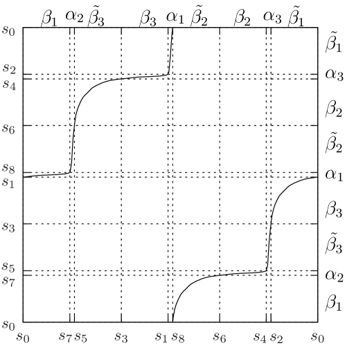
Figure 6: Plotting the $\sigma$ function with a grid of the partition points $s_{i}$ we can read off which piece of the curve is in contact (in the $\sigma$ direction) with which other piece. For example starting at the top with $\alpha_{1}$ we see that $\sigma$ maps its parameter-interval to the parameter-interval of $\tilde{\beta_{1}}$ on the right, which itself gets mapped from top $\tilde{\beta_{1}}$ to $\beta_{3}$ on the right and so on (see Lemma 3).

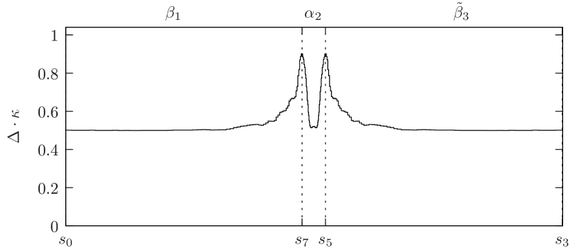
Figure 7: The curvature $\kappa$ of $\gamma_{3_{1}}$ is confined to $[0,1/\Delta]$. Consequently the graph shows $\kappa\cdot\Delta$. Since $\kappa$ is three-periodic, for greater detail we show only one third of the interval. The maximal curvature is attained at $s_{7}$ and $s_{5}$.

Figure 8: Since numerical experiments find that $\sigma^{i+9}-\sigma^{i}$ converges point-wise to $0$ for $i\to\infty$ we conjecture that the cycle $b_{9}$ acts as an attractor, i.e. $(\sigma^{9i}(s),\sigma^{9i+1}(s),\ldots,\sigma^{9i+8}(s))$ converges to $b_{9}$ up to a cyclic permutation. Notice that the convergence is only point-wise and cannot be uniform since $\sigma$ is continuous; with enough samples we would see large spikes after each $s_{i}$ as behind $s_{6}$ and $s_{8}$ above.

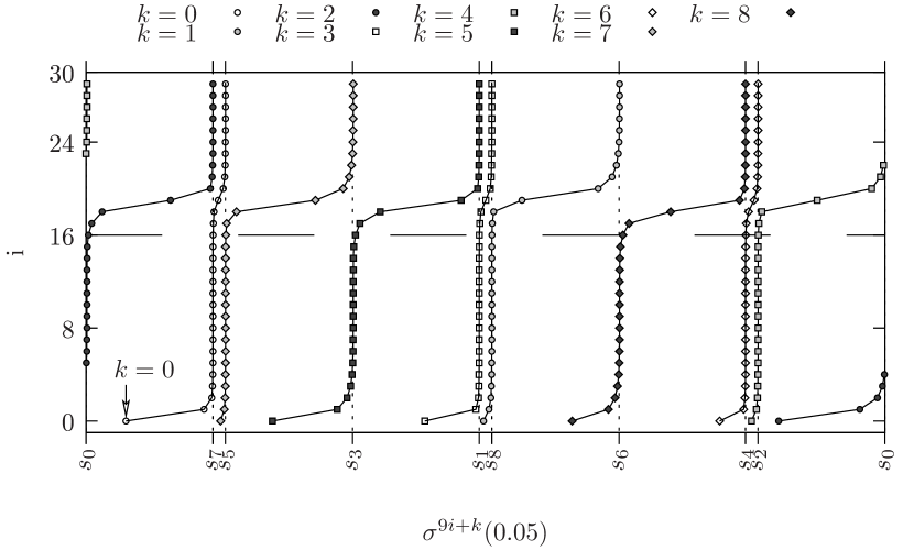
Figure 9: The cycle $b_{9}$ seems to be an attractor: starting at the arbitrary point $t=0.05$ the sequence $\sigma^{9i}(t)$ seems to converge to $s_{7}$ for growing $i$. After $i>16$ iterations, presumably, errors in the approximation and the numerics add up and $\sigma^{9\cdot 18}(t)$ is in the next interval $(s_{7},s_{5})$. Starting from $\sigma^{k}(t)$ in other intervals shows a similar behavior.

Taking a second look at Figure 4 it looks like $\sigma^{n}$ is approaching a step function as $n$ increases. What are the accumulation points of the sequence $\{\sigma^{i}(t)\}_{i}$ as a function of $t\in\mathbb{S}$? Looking at $(\sigma^{i}(t),\sigma^{i+1}(t),\ldots,\sigma^{i+8}(t))$ for arbitrary $t\in\mathbb{S}$ it seems to converge to $b_{9}$ up to a cyclic permutation for $i$ large enough, i.e. $b_{9}$ contains the accumulation-points of the above sequence. Figure 8 shows some numeric values of $\sigma^{i+9}-\sigma^{i}$ which seems to converge point-wise to $0$ for $i\to\infty$. An arbitrary point $t$ between neighboring points $s_{l}$ and $s_{r}$ gets by each application of $\sigma^{9}$ repelled from the left by $s_{l}$ and attracted to the right by $s_{r}$ (see Figure 9). Note that the attactor has a direction that is induced by the chirality of the trefoil (left or right-handed) and the choice of the contact function $\sigma$ made in Definition 3.

Conjecture 3 (Attractor).

Let $b_{n}\in(\mathbb{S})^{n}$ be a cycle. We call $b_{n}$ an attractor if for any $t\in\mathbb{S}$ and fixed $k\in\{0,\ldots,n-1\}$ the $n$-tuple $(\sigma^{i}(t),\sigma^{i+1}(t),\ldots,\sigma^{i+n-1}(t))$ converges to a cyclic permutation of $b_{n}$ for $j\to\infty$ with $i=nj+k$. The $b_{9}$ cycle of Conjecture 2 is an attractor.

The existence of an attractor rules out the existence of other cycles:

Lemma 4.

Assume $\gamma_{3_{1}}$ has a contact function $\sigma$ as in Definition 3 and let $b_{n}\in(\mathbb{S})^{n}$ be a $n$-cycle as in Conjecture 2. Then $b_{n}$ is an attractor in the sense of Conjecture 3 iff there is no other $n$-cycle on $\gamma_{3_{1}}$.

Proof.

Assume that $c_{n}=(t_{0},\sigma(t_{0}),\ldots,\sigma^{n-1}(t_{0}))$ is a $n$-cycle different from $b_{n}$. Then $\sigma^{n}(t_{0})=t_{0}$ and $b_{n}$ cannot be an attractor.

To prove the converse, let $b_{n}=(s_{0},\ldots,s_{n-1})$ be an $n$-cycle and consider $\sigma^{n}$ as a continuous, injective and orientation preserving map from $[s_{k},s_{l}]\subset\mathbb{R}$ to itself, where $l$ and $k$ are such that $s_{l}$ and $s_{k}$ are neighboring, i.e. $s_{i}\not\in(s_{k},s_{l})$ for all $i$. The cycle $b_{n}$ is an attractor iff for all $x\in(s_{k},s_{l}]$ the sequence $x_{i}:=\sigma^{ni}(x)$ converges to $s_{l}$ as $i\to\infty$. Since $\sigma$ is orientation preserving we have $x_{i}\leq x_{i+1}$, i.e. the sequence is monotone. Assume that $b_{n}$ is not an attractor, i.e. for some $x$ the sequence $\{\sigma^{ni}(x)\}_{i}$ is bounded away from $s_{l}$, then it must converge to some smaller value $c<s_{l}$. By continuity of $\sigma^{n}$ it follows that $c$ is a fixed point. Therefore $c_{n}:=(c,\sigma^{1}(c),\sigma^{2}(c),\ldots,\sigma^{n}(c))$ is a closed $n$-cycle different from $b_{n}$. ∎

As mentioned above, by concatenation, a minimal cycle gives rise to a series of larger, non-minimal cycles: For an $n$-cycle $a_{n}=(x_{0},\ldots,x_{n-1})$ we define an $nk$-cycle

$$a^{k}_{n}:=(\underbrace{x_{0},\ldots,x_{n-1},\ldots,x_{0},\ldots,x_{n-1}}_{k\text{ times}}).$$

Proposition 1.

Assume $\gamma_{3_{1}}$ has a contact function $\sigma$ as in Definition 3 and let $b_{n}\in(\mathbb{S})^{n}$ be a minimal $n$-cycle as in Conjecture 2 and an attractor in the sense of Conjecture 3. Then $b_{n}$ is the only minimal cycle and all other cycles are multiples of $b_{n}$.

Proof.

Let $c_{m}$ be a $m$-cycle different from $b_{n}$. We claim $c_{m}=b^{k}_{n}$ and $m=kn$ for some $k\in\mathbb{N}$.

If $b_{n}$ is an attractor, then $b^{i}_{n}$ is also an attractor for $i\in\mathbb{N}$. Let $g$ be the greatest common divisor of $n$ and $m$, so $l=mn/g$ is their least common multiple. Then $b_{n}^{m/g}$ is an attractor and an $l$-cycle, but $c_{m}^{n/g}$ is an $l$-cycle as well and Lemma 4 implies $b^{m/g}_{n}=c^{n/g}_{m}$. Since $b_{n}$ was minimal, this is only possible if $c_{m}=b^{k}_{n}$ for some $k\in\mathbb{N}$. ∎

Lemma 4 and Proposition 1 fit well with our numerical observation. We find only one possible cycle and it seems to be an attractor.

4 Conclusion

We have presented numerical and esthetical compelling evidence for the existence of a closed nine-cycle in the contact chords of the ideal trefoil knot. Enforcing symmetry based on a Fourier representation turned out to be essential to observe this feature. The cycle leads to a partitioning of the trefoil. Only two segments of the curve have to be considered, the remaining parts of the trefoil can be reconstructed by symmetry. For other contact chord paths, after enough iterations, it seems that they eventually converge to the nine-cycle. So the closed cycle acts as an attractor for all other billiards.

Preliminary numeric experiments by E. Starostin suggest closed cycles in ideal shapes of knots with a higher number of crossings as well. The interesting cases remain however inconclusive, since these knot shapes are believed to be much less ideal than the trefoil. Closed cycles in these knots might then also suggest a natural partitioning of the curves, therefore improving the understanding of these knots.

In the $\mathbb{S}^{3}$ setting [11] suggested a candidate trefoil for ideality to the problem of maximizing thickness. Each point on the $\mathbb{S}^{3}$ trefoil is in contact with two other points on the curve. Following the contact great-arcs (in $\mathbb{S}^{3}$) five times forms a circle, i.e. a 5-cycle.

The numerical computations suggest at least two new challenges: First, can we get new insights about the ideal trefoil assuming the existence of a nine-cycle? And second, can we prove, under some reasonable hypothesis, that the ideal trefoil or even every ideal knot has closed contact cycles?

5 Acknowledgements

Research supported by the Swiss National Science Foundation SNSF No. 117898 and SNSF No. 116740. We would like to thank E. Starostin and J.H. Maddocks for interesting discussions and helpful comments.

References

- [1] T. Ashton, J. Cantarella, M. Piatek, E.J. Rawdon, Knot Tightening by Constrained Gradient Descent. arXiv:1002.1723v1 [math.DG], (2010).
- [2] T. Ashton, J. Cantarella, M. Piatek, E.J. Rawdon, Self-contact sets for 50 tightly knotted and linked tubes. math.DG/0508248 in preparation, (2005).
- [3] J. Baranska, S. Przybyl, P. Pieranski, Curvature and torsion of the tight closed trefoil knot, Eur. Phys. J. B 66, 547–556 (2008).
- [4] G.D. Birkhoff, Dynamical Systems, American Mathematical Society (1927).
- [5] J. Cantarella, J.H.G. Fu, R.B. Kusner, J.M. Sullivan, N.C. Wrinkle, Criticality for the Gehring link problem, Geom. Topol. 10 (2006), 2055–2116.
- [6] J. Cantarella, R.B. Kusner, J.M. Sullivan, On the minimum ropelength of knots and links. Inv. math. 150 (2002), 257–286.
- [7] J. Cantarella, M. Piatek, E. Rawdon, Visualizing the tightening of knots In VIS ’05: Proceedings of the 16th IEEE Visualization (2005), 575–582.
- [8] M. Carlen, Computation and visualization of ideal knot shapes, PhD thesis No. 4621, EPF Lausanne (2010), http://library.epfl.ch/theses/?display=detail&nr=4621.
- [9] M. Carlen, H. Gerlach, Fourier approximation of symmetric ideal knots, Journal of Knot Theory and Its Ramifications (submitted July 2010), http://lcvmwww.epfl.ch/~lcvm/articles/127/info.html.
- [10] M. Carlen, B. Laurie, J.H. Maddocks, J. Smutny, Biarcs, global radius of curvature, and the computation of ideal knot shapes in J.A. Calvo, K.C. Millett, E.J. Rawdon, A. Stasiak (eds.), Physical and Numerical Models in Knot Theory, Ser. on Knots and Everything 36, World Scientific, Singapore (2005), 75–108.
- [11] H. Gerlach, Ideal Knots and Other Packing Problems of Tubes, PhD thesis No. 4601, EPF Lausanne (2010), http://library.epfl.ch/theses/?display=detail&nr=4601.
- [12] O. Gonzalez, J.H. Maddocks, Global Curvature, Thickness and the Ideal Shapes of Knots, Proc. Natl. Acad. Sci. USA 96 (1999), 4769–4773.
- [13] O. Gonzalez, J.H. Maddocks, F. Schuricht, H. von der Mosel, Global curvature and self-contact of nonlinearly elastic curves and rods, Calc. Var. 14 (2002), 29–68.
- [14] M. Carlen, H. Gerlach, Ideal knots, numerical data http://lcvmwww.epfl.ch/~lcvm/articles/T10/data/, (2010).
- [15] V. Katritch, J. Bednar, D. Michoud, R.G. Scharein, J. Dubochet, A. Stasiak, Geometry and physics of knots, Nature 384 (1996), 142–145.
- [16] B. Laurie, Annealing Ideal Knots and Links: Methods and Pitfalls, in [23], 42–51.
- [17] M. Carlen, libbiarc webpage, http://lcvmwww.epfl.ch/libbiarc/, used version 96c4cef03910, (2010).
- [18] R.A. Litherland, J. Simon, O.C. Durumeric, E.J. Rawdon, Thickness of Knots, Topology and its Applications 91(3) (1999), 233–244.
- [19] P. Pieranski, S. Przybyl, In Search of the Ideal Trefoil Knot, in Physical Knots, Eds. J. Calvo, K. Millett, E.J. Rawdon, and A. Stasiak, World Scientific (2001), 153–162.
- [20] Pieranski P., In Search of Ideal Knots, in [23], 20–41.
- [21] J. Smutny, Global radii of curvature and the biarc approximation of spaces curves: In pursuit of ideal knot shapes, PhD thesis No. 2981, EPF Lausanne (2004), http://library.epfl.ch/theses/?display=detail&nr=2981.
- [22] E. Starostin, A constructive approach to modelling the tight shapes of some linked structures Forma 18 (4), (2003) 263–293.
- [23] A. Stasiak, V. Katritch, L.H. Kauffman (Eds), Ideal knots, Ser. Knots Everything 19, World Sci. Publishing, River Edge, NJ, (1998).