Energy-Optimal Scheduling in Low Duty Cycle Sensor Networks

Abstract

Energy consumption of a wireless sensor node mainly depends on the amount of time the node spends in each of the high power active (e.g., transmit, receive) and low power sleep modes. It has been well established that in order to prolong node’s lifetime the duty-cycle of the node should be low. However, low power sleep modes usually have low current draw but high energy cost while switching to the active mode with a higher current draw. In this work, we investigate a MaxWeight-like opportunistic sleep-active scheduling algorithm that takes into account time- varying channel and traffic conditions. We show that our algorithm is energy optimal in the sense that the proposed ESS algorithm can achieve an energy consumption which is arbitrarily close to the global minimum solution. Simulation studies are provided to confirm the theoretical results.

I Introduction

Wireless sensor network consists of many battery operated nodes with limited processing and wireless communicating abilities. They are used in many different areas such as military, scientific research or medical diagnostics. Since sensor networks are uniquely identified by their requirement of operation for a long period without outside intervention, energy consumption is a primary concern. Unnecessary energy consumption can be caused from the implementation at PHY layer. For instance, keeping the sensor nodes in active all the time is one of the main inefficiency. Furthermore, energy unaware scheduling algorithms employed at MAC or above layers is the another reason for the unnecessary energy consumption.

A particularly important strategy is to minimize wasted energy due to idle listening, in other words, operate the nodes with low duty cycles [1]. Duty cycle is defined as the proportion of time the node stays active in its lifetime. Thus, it is necessary to reduce the duty cycle in order to resolve this conflict. A sensor node consumes energy while transmitting, receiving and sleeping Also, switching between these three modes is the another issue and the sensors require extra time and spend extra energy for switching. In most prior works, it was assumed that the switching energy is negligible compared to the energy spent in other modes. It is recently observed that, this assumption does not hold in low duty cycle sensor networks [2]. For example, in [2] for CC1010 type sensor nodes, while the switching energy from sleep mode to transmit mode is given as 47.75 $\mu J$ for the switching time is 0.7 ms, the energy consumed during the transmission taken 0.7 ms is equal to 124.8$\mu J$. This measurement shows that the switching energy is crucial and should be taken into account for any energy efficient scheduling algorithm.

In the literature, there are many scheduling algorithms that have been developed for network stability problem with strong theoretical results. Tassiulas et al. in [3] first introduced the design of backpressure algorithms based on Lyapunov drift techniques to achieve network stability and the authors in [4] developed algorithm which deals with performance optimization and queue stability problems simultaneously in a unified framework. There exists also a rich literature on using Lyapunov drift optimization for solving problems of energy optimization in wireless networks. In this paper, one of our objectives is to show the significance of switching energy in the design of scheduling policy.

II Related Works

There are many works that offer low energy consumption in the literature [5], [6], [7], [8]. In all these works, the proposed algorithms and experiments have been designed by only taking into account the energy consumption in the active and sleep modes but they have not considered the consumed energy during switching from one state to another. In addition, none of these works deals with the network stability problem with the objective of minimum energy. In [9], the authors have proposed wireless sensor network protocols that take into account the source of energy consumptions in a network simulation model. They have also mentioned about switching energy but leaved it as an open research area. The study in [10] have considered switching energy cost since it has been observed that significant energy consumption occurs when switching from sleep mode to the active mode. On the other hand, in some studies like [11] it has been stated that the energy cost of switching is small. Generally, it is common to ignore switching energy in the literature. There are also various approaches proposed for designing duty cycling protocols [12], [2], [13], for sleep mode protocols [14] and for routing protocols [15], [16]. All of these works try to maximize the lifespan or the utility of the network without considering the network stability problem.

The works in [17], [18] and [19] are the most important ones considering network stability issue for wireless sensor network. In [17], the authors proposed a back pressure algorithm designed using a Lyapunov drift based optimization framework using the receiver capacity model. However, they did not aim to minimize the average energy consumption. An optimal control algorithm for rechargeable wireless sensor nodes is proposed in [18] where the objective function is maximize the network utility subject to stability. In [19], the authors proposed a scheduling algorithm based on Lyapunov optimization theory in order to minimized the consumed energy while maintaining the network stability. However, they do not consider low duty cycle sensor networks.

In this paper, we develop a throughput optimal scheduling algorithm based on the Lyapunov drift framework which considers not only minimizing energy but also sustaining network stability for low duty cycle sensor networks. Our energy switching and scheduling (ESS) algorithm is energy optimal in the sense that it minimizes the overall expected energy consumed in the network over all scheduling algorithms and remains throughput optimal. The proposed ESS algorithm prolongs the lifetime compared to the benchmark algorithm which does not consider switching energy. Therefore, our proposed ESS algorithm is more favorable for scheduling in low duty cycle wireless sensor networks.

The rest of the paper is organized as follows. Section III describes the system model and problem formulation. The proposed ESS algorithm is introduced in Section IV. Lyapunov optimization technique which is used to show the performance and the optimality of ESS algorithm and a distributed algorithm are given in Section V. We present our simulation result in Section VI and Section VII concludes this paper.

III System Model and Problem Statement

III-A System Model

We consider an uplink scenario where $N$ sensor nodes sense the environment and transmit to a base station. The network is operated in slotted time $t=0,1,2,...$ where slot $t$ corresponds to the time interval $[t,t+1)$. The node channels are time-varying and the instantaneous channel state is represented by $\mathbf{M}(t)$ and assume it is i.i.d distributed over a finite set $\mathcal{M}$, $\mathbf{M}(t)\in\mathcal{M}$. We also define $\pi_{m}\triangleq Pr(\mathbf{M}(t)=m)$ as steady state probability of being in channel state $m$ at time slot $t$. Channels are assumed to hold their state within one time slot. The data rate of node $n$ during slot $t$ is represented by $\mu_{n}(I_{n}(t),M_{n}(t))$ (in units of packets/slot) where $M_{n}(t)$ is the channel state of node $n$ and $I_{n}(t)=1$, whenever node $n$ is selected as a transmitting node at time $t$, and $I_{n}(t)=0$ otherwise. We assume that $\mu_{n}(I_{n}(t),M_{n}(t))$ is upper bounded with $\mu_{n}(I_{n}(t),M_{n}(t))\leq\mu_{max}$. For ease of notation, we use $\mu_{n}(t)$ instead of $\mu_{n}(I_{n}(t),M_{n}(t))$ in the rest of the paper.

At each time slot $t$, the number of new packets generated by node $n$ is denoted by $R_{n}(t)$. We assume that $R_{n}(t)$ is i.i.d for each time slot with an average rate of $\lambda_{n}$, and it is upper bounded with $R_{n}(t)\leq R_{max}$. We define the network admission rate vector as $\boldsymbol{\lambda}=\{\lambda_{1},\lambda_{2},...,\lambda_{N}\}$ where $\lambda_{n}$ is the average exogenous arrival rate of node $n$. Let $\Lambda$ be the network capacity region, i.e., the set of all feasible admission rate vectors that the network can support.

III-B Notations

In our network model, there are $K$ the sensor nodes which can be in active or sleep modes at a particular time slot. Therefore, the node $n\in N$ where $N$ represents the set of all nodes has an action space denoted as $A=\{0,1\}$. We denote $s$ as the action taken by any node and $s=0$ and $s=1$ represent the sleep and active modes respectively. The sensor can also switch from active to sleep or vice versa and we denote $sw\in\{01,10\}$ as the switching action where $sw=01$ and $sw=10$ represent the switching from sleep to active and active to sleep modes respectively. In addition, we denote the set of all sleep and active nodes as $Sl$ and $Ac$ respectively at a given time slot.

III-C Problem Formulation

We begin with a definition of network stability. Let $Q_{n}(t)$ be the queue backlog of node $n$ at time slot $t$.

Definition 1

A queue is strongly stable if

$$\limsup_{t\rightarrow\infty}\frac{1}{t}\sum_{\tau=0}^{t-1}\mathbb{E}(Q_{n}(t))<\infty$$ (1)

Moreover, if every queue in the network is stable then the network is called stable. The system stability region is the the closure of the convex hull of all arrival rate points for which there exists a feasible scheduling policy that achieves system stability [4].

We consider an energy consumption model defined as follows. At the beginning of transmission, each sensor has a full battery of $E$. In each time slot, a particular node can be either in active or sleep modes according to its remaining energy, queue backlog and channel condition. During the sleep mode, the node is unable to transmit packets. However, packets continue to be generated by the node, and they are queued until the node has the opportunity to transmit them. Let $e_{s}^{n}(t)$ be the energy consumed by node $n$ when it is in mode $s\in\{0,1\}$ at time $t$. When the node is active, it consumes an energy $c_{n}(t)$ that depends on the current draw of active mode by the circuit, and how much time the node spends in active mode. Also, the energy needed for packets transmission should be included to the total energy expenditure when the node is selected to transmit. Then at time $t$, the total energy consumption by node $n$ in active mode becomes $e_{1}^{n}(t)=c_{n}(t)+\mu_{n}(t)\alpha_{n}$ where $\alpha_{n}$ denotes the energy spent for a packet transmission. Furthermore, if a node switches from sleep-to-active or active-to-sleep modes, then the switching energy denoted as $e_{sw}^{n}(t)$ is consumed. The values of energy costs are given in Section VI. Hence, the overall energy spent by node $n$ during time slot $t$ is given by:

$$H^{n}(t)=\sum_{s\in A}\textrm{e}_{s}^{n}(t)+e_{sw}^{n}(t)\qquad s\in\{0,1\}.$$ (2)

and the total energy consumption in the network at time slot $t$ is obtained by summing over all nodes in the system,

$$H(t)=\sum_{n}\sum_{s\in A}\textrm{e}_{s}^{n}(t)+\sum_{n}e_{sw}^{n}(t)\qquad s\in\{0,1\}$$ (3)

Define the time average expected total energy consumption as,

$$\overline{H}=\limsup_{t\rightarrow\infty}\frac{1}{t}\sum_{\tau=0}^{t-1}\mathbb{E}\left[\sum_{n}\sum_{s}\textrm{e}_{s}^{n}(\tau)+\sum_{n}e_{sw}^{n}(\tau)\right]$$ (4)

The expectation is with respect to the randomness that arises from channel variations and arrival process and possibly from random stationary switching policy. The overall energy consumption during time $t$ is upper bounded by a finite value since all sensors have a limited battery power and thus, without lost of generality, we assume that the following is satisfied at every time slot,

$$\sum_{n}H^{n}(t)\leq H_{max},\;\forall t$$ (5)

We are interested in minimizing the total average energy consumption in the network while keeping the queue sizes of the sensor nodes bounded. Then, our optimization problem can be formalized as follows,

$$\min\quad \overline{H}$$ (6)

$$s.t.\quad$$ network stability. (7)

IV Energy-Aware Switching and Scheduling (ESS) Algorithm

In this section, we introduce our energy aware sleep-active scheduling algorithm which asymptotically minimizes the average network energy consumption subject to the network stability. Furthermore, the proposed algorithm is shown to be throughput optimal meaning that the algorithm can guarantee the network stability for all feasible network admission rates.

At each time slot, the proposed Energy-aware Switching and Scheduling (ESS) algorithm determines the energy modes of operation for each sensor nodes and selects the transmitting node which maximizes the following:
ESS

$$\max_{n\in Ac,s}\quad Q_{n}(t)\mu_{n}(t)-V\textrm{e}_{sw}^{n}(t)-V\sum_{s\in A}\textrm{e}_{s}^{n}(t).$$ (8)

In (8), $V>0$ is a system parameter and shows the well-known delay-energy tradeoff [4]. For very large value of $V$ we can push the average energy consumed by ESS algorithm arbitrarily close to the global minimum energy. However, in that case in order to maximize (8) nodes stay in the sleep mode most of the time, and consequently, the queue sizes increase.

Remark 1: As it is seen in (8), ESS algorithm is different from the Max Weight algorithm, and the algorithm proposed in [19] since ESS not only considers the energy consumption in sleep and active modes but also takes into account the switching energy cost. It is shown in simulation studies that this cost cannot be ignored and has significant in the life time of the network.

Remark 2: The basic properties of ESS algorithm are as follows. In each time slot $t$ at most one node is active, and this node transmits. The active node continues to transmit in consecutive slots until some other node is the maximizer of (8). On the other hand, the rest of the nodes stay in the sleep mode and their queue backlogs increase. Once the queue backlog of a sleeping node is sufficiently high in order to maximizes (8) then this node is selected to transmit. Furthermore, if all of the queue backlogs are low, the nodes choose to stay in the sleep mode. Thus, the system can be in the idle state where no nodes choose to be active during some of the time slots.

Lemma 1

ESS satisfies the following properties.

1. Sensor nodes transmit in a bursty fashion, i.e., transmit multiple packets once they capture the channel.

2. The system operation is non-work conserving, i.e., there are idle slots when no sensor node transmits even if their backlog is non-empty.

Proof:

For notational brevity, let $n$ and $m$ represent the active and sleeping nodes respectively and their corresponding queue sizes are denoted as $Q_{n}(t)$ and $Q_{m}(t)$ at time slot $t$. If the active node $n$ prefers to be again active during next time slot $t+1$, it does not need to change its energy mode and there will be no switching energy cost ($e^{n}_{sw}(t)=0$). Thus, its weight is equal to $Q_{n}(t)\mu_{n}(t)-Ve_{1}^{n}(t)$ according to (8). On the other hand, if it switches its mode from active to the sleep, then it obtains the weight which is equal to $-Ve_{0}^{n}(t)-Ve_{01}^{n}(t)$ since it cannot transmit in sleeping mode and $\mu_{n}(t)=0$ and also it pays a switching energy cost which is equal to $e^{n}_{10}(t)>0$. Therefore, the node $n$ prefers to stay in active mode if and only if the weight obtained in active mode exceeds the weight resulting from switching to sleep mode. In other words, the following inequality should be hold.

$$-Ve_{0}^{n}(t)-Ve_{10}^{n}(t)<Q_{n}(t)\mu_{n}(t)-Ve_{1}^{n}(t)$$

Thus

$$\frac{V(e_{1}^{n}(t)-e_{0}^{n}(t)-e_{10}^{n}(t))}{\mu_{n}(t)}<Q_{n}(t)$$ (9)

Furthermore, since ESS algorithm aims to maximize (8), the node $n$ continues to be active and transmits if and only if it is the maximizer of (8).

$$\max_{b\in Sl}\left[Q_{b}(t)\mu_{b}(t)-Ve_{01}^{b}(t)-Ve_{1}^{b}(t)\right]$$

$$<Q_{n}(t)\mu_{n}(t)-Ve_{1}^{n}(t)$$ (10)

Therefore, as long as inequalities (9) and (10) hold, active sensor node transmits in a bursty fashion and the other nodes do not change their energy modes. This completes the first part of Lemma 1.

On the other hand, if the sleeping node $m$ prefers to stay in sleep mode during next slot $t+1$, according to equation (8) its weight is $-Ve_{0}^{m}(t)$ since it cannot transmit then $\mu_{m}(t)=0$ and there will no switching cost $e^{m}_{sw}(t)=0$. If it switches to active mode and transmit, then it obtains the weight which is equal to $Q_{m}(t)\mu_{m}(t)-Ve_{01}^{m}(t)-Ve_{1}^{m}(t)$. Therefore, the node $m$ node continues to stay in sleep mode if and only if its queue sizes is not large enough to cover the reward being in sleep mode. In other words, it stays in sleep mode as long as the following inequality holds,

$$-Ve_{0}^{m}(t)>Q_{m}(t)\mu_{m}(t)-Ve_{01}^{m}(t)-Ve_{1}^{m}(t)$$

Thus

$$\frac{V(e_{1}^{m}(t)+e_{01}^{m}(t)-e_{0}^{m}(t))}{\mu_{m}(t)}>Q_{m}(t)$$ (11)

Similarly, the active node prefers to switch to sleep mode, if its backlog is not large enough to maximize (8). Therefore, the system is idle if the following inequalities are satisfied

$$Q_{n}(t)< \frac{V(e_{1}^{n}(t)-e_{0}^{n}(t)-e_{10}^{n}(t))}{\mu_{n}(t)} \forall n\in Ac$$ (12)

$$Q_{m}(t)< \frac{V(e_{1}^{m}(t)+e_{01}^{m}(t)-e_{0}^{m}(t))}{\mu_{m}(t)} \forall{m}\in Sl$$ (13)

∎

V Throughput optimality of ESS

Despite the fact that (6)-(7) is a convex optimization problem, a direct solution is generally overly complicated since the arrival rates resulting network stability does not admit in general a simple characterization. Fortunately, we can use the framework of [4], and obtain a dynamic scheduling policy that operates arbitrarily closely to the optimal point. This is obtained in two steps: first, a dynamic scheduling policy that achieves the stability of transmission queues whenever the arrival rates are inside the stable network operating region is obtained. Second, we define a stationary randomized algorithm and compare the randomized policy with our ESS algorithm.

V-A Optimal Stationary Randomized Algorithm

Now, we present a stationary randomized algorithm which is used to prove the stability property and throughput optimality of ESS algorithm. The randomized algorithm schedules the nodes according to a stationary, and possibly randomized function of only the data rates and it is independent of the queue backlog. Let us denote the stationary randomized algorithm as $RND$. With $RND$ algorithm, the switching decision is determined by a Markovian process with two states; sleep and active. We denote the transition probabilities from active to sleep states and from sleep to active states as $p_{10}$ and $p_{01}$ respectively. The steady-state probabilities of the active and sleep modes are denoted as $\pi_{a}$ and $\pi_{s}$ respectively. We assume that channel processes are ergodic with steady-state probabilities $\pi_{k}$ where $k$ is describing the channel state in a finite set, ${k}\in\{1,2,...,M\}$. The following theorem specifies the minimum energy required for stability, among the class of stationary policies that randomly decides on sleep-active modes and transmit scheduling.

Theorem 1

If arrival rate vector is strictly in the capacity region $\boldsymbol{\lambda}\in\Lambda$, then the minimum energy that can stabilize the network is denoted by $h^{*}$ and it is equal to the solution of the following optimization problem that is defined in terms of transition probabilities $(p^{n}_{ij})_{k}$ for $(i,j)\in\{0,1\}$, steady-state probabilities $(\pi_{l}^{n})_{k}$ for $l\in\{a,s\}$ and transmission probabilities $(\pi_{tr}^{n})_{k}$ at channel state $k\in\mathbf{M}$.

$$\min\quad \sum_{k\in\mathbf{M}}\pi_{k}\sum_{n}(p_{10}^{n})_{k}(\pi_{s}^{n})_{k}+(p_{01}^{n})_{k}(\pi_{a}^{n})_{k}e_{sw}^{n}+(\pi_{s}^{n})_{k}e_{0}^{n}$$

$$\qquad\quad\quad\;+(\pi_{a}^{n})_{k}(c^{n}(t)+(\pi_{tr}^{n})_{k}(\mu_{n})_{k}\alpha_{n})$$

$$s.t.\quad \sum_{k\in\mathbf{M}}\pi_{k}(\pi_{a}^{n})_{k}(\pi_{tr}^{n})_{k}(\mu_{n})_{k}\geq\lambda_{n}\quad\forall n$$

$$\sum_{k}(\pi_{p}^{n})_{k}\leq 1\qquad\;\;\;\forall p\in\{a,s\},\quad\forall n$$

$$\sum_{n\in Ac}(\pi_{tr}^{n})_{k}\leq 1\quad\qquad\quad\forall k$$

where $(\mu_{n})_{k}$ is the data rate of node $n$ at channel state $k\in\mathbf{M}$.

Proof:

The proof follows the same line of logic as the proof given [20]. The optimization problem above can be solved since the set of channel state is finite and the energy set is compact. Thus, we can achieve the minimum energy by a randomized algorithm which decides the switching decision with probabilities $(p^{n}_{ij})_{k}$ and selects the transmission node with probability $(\pi_{tr}^{n})_{k}$.

Since $\boldsymbol{\lambda}$ lies in the interior of the network capacity region $\Lambda$, it follows that there exists a small positive $\boldsymbol{\epsilon}>0$ such that $\boldsymbol{\lambda}+\boldsymbol{\epsilon}\in\Lambda$. Then, there exist a stationary policy which stabilizes the network while providing a data rate of

$$\mathbb{E}(\boldsymbol{\hat{\mu}}(t))\geq\boldsymbol{\lambda}+\boldsymbol{\epsilon},$$ (14)

where $\boldsymbol{\hat{\mu}}$ is the transmission rate induced by the randomized policy. Let $h^{*}(\epsilon)$ be the minimum energy consumed by such policy. Since expected transmission rate is greater than the arrival rate, the network is stable. In addition, since $h^{*}(\epsilon)$ is the minimum energy required to stabilize the network with arrival rate $\boldsymbol{\lambda}+\boldsymbol{\epsilon}$, any mixed strategy results in higher energy consumption. Therefore, it is obvious that

$$h^{*}\leq h^{*}(\epsilon)\leq\left(1-\frac{\epsilon}{\epsilon_{max}}\right)h^{*}+\frac{\epsilon}{\epsilon_{max}}h^{*}(\epsilon_{max})$$ (15)

where $\epsilon_{max}$ is the largest scalar where $\lambda_{n}+\epsilon_{max}\in\Lambda$. When $\epsilon=\epsilon_{max}$, nodes consume much more energy to stabilize the queues. Therefore, $h^{*}(\epsilon_{max})\geq h^{*}(\epsilon)\;\forall\epsilon$. It follows that $h^{*}(\epsilon)\rightarrow h^{*}$ as $\epsilon\rightarrow 0$.
∎

Theorem 1 indicates that the minimum energy consumption for stability is achieved among the class of stationary policies that measure the current channel state $\mathbf{M}(t)$, and then randomly decides switching and selects the user which transmits.

V-B Analysis of ESS

In our work, we use Lyapunov drift and optimization tools  [4] to show the optimality of ESS algorithm. The advantage of this tool is the ability to deal with performance optimization, and queue stability problems simultaneously in a unified framework. For node $n$ the queue dynamics is given by

$$Q_{n}(t+1)=\max(Q_{n}(t)-\mu_{n}(t),0)+R_{n}(t)$$ (16)

We can write the following inequality by using the fact $([a]^{+})^{2}\leq(a)^{2},\quad\forall a$:

$$Q^{2}_{n}(t+1)\leq Q^{2}_{n}(t)$$ (17)

$$+(\mu_{max})^{2}+(R_{max})^{2}-2Q_{n}(t)[\mu_{n}(t)-R_{n}(t)]$$

Let $\textbf{Q}(t)=(Q_{1}(t),Q_{2}(t),...,Q_{N}(t))$ be a queue vector and define the following quadratic Lyapunov function

$$L(\mathbf{Q}(t))\triangleq\frac{1}{2}\sum_{n=1}^{N}(Q_{n}^{2}(t))$$ (18)

and the conditional Lyapunov drift is

$$\Delta(t)\triangleq\mathbb{E}\left\{L(\mathbf{Q}(t+1))-L(\mathbf{Q}(t))|\mathbf{Q}(t)\right\}$$ (19)

Then, by using (17) Lyapunov drift of the system satisfies the following inequality at every time slot,

$$\Delta(t)\leq B-\sum_{n}\mathbb{E}\left\{Q_{n}(t)(\mu_{n}(t)-R_{n}(t))|\mathbf{Q}(t)\right\},$$ (20)

where

$$B=\frac{K}{2}((\mu_{max})^{2}+(R_{max})^{2}).$$ (21)

In addition, we define a cost function $\mathbb{E}(H(t)|\mathbf{Q}(t))$ as the expected total energy consumption during time slot $t$. After adding the cost function multiplied by $V$ to both sides of (20), we have the following.

$$\Delta(t)+V\mathbb{E}(H(t)|\mathbf{Q}(t))$$

$$\leq B-\sum_{n}\mathbb{E}\left\{Q_{n}(t)(\mu_{n}(t)-R_{n}(t))|\mathbf{Q}(t)\right\}+V\mathbb{E}(H(t)|\mathbf{Q}(t))$$

$$\leq B-\sum_{n}\mathbb{E}\left\{Q_{n}(t)\mu_{n}(t)|\mathbf{Q}(t)\right\}+V\sum_{n}\sum_{s}\mathbb{E}\left\{\textrm{e}_{s}^{n}(t)|\mathbf{Q}(t)\right\}$$

$$+V\sum_{n}\mathbb{E}\left\{\textrm{e}_{sw}^{n}(t)|\mathbf{Q}(t)\right\}$$

$$\leq B-\underbrace{\sum_{n}\mathbb{E}\left\{Q_{n}(t)\mu_{n}(t)-V\textrm{e}_{sw}^{n}(t)-V\sum_{s}\textrm{e}_{s}^{n}(t)|\mathbf{Q}(t)\right\}}_{RHS^{ESS}}$$ (22)

where $RHS^{ESS}$ is the right hand side of  (22). It is now straightforward to see that ESS algorithm minimizes $RHS^{ESS}$ over all possible stationary algorithms.

We now present a fact given in [4] that will be used to prove that ESS is throughput optimal.

Theorem 2

(Lyapunov Stability) For scalar valued function $g(.)$ for which the minimum value is equal to $g^{*}$, If there exists positive constants $V,\epsilon,B$ such that for all time slots $t$ and all backlog vectors $\mathbf{Q}(t)$, the Lyapunov drift satisfies

$$\Delta(t)+V\mathbb{E}(g(t)|\mathbf{Q}(t))\leq B-\epsilon\sum_{i=1}^{N}Q_{i}(t)+Vg^{*},$$ (23)

then the system is stable and the time average backlog satisfies:

$$\limsup_{T\rightarrow\infty}\frac{1}{T}\sum_{t=0}^{T-1}\sum_{i=1}^{N}\mathbb{E}\{Q_{i}(t)\}\leq\frac{B+Vg^{*}}{\epsilon}$$

Theorem 3

The proposed ESS algorithm is throughput optimal.

Proof:

Clearly, the RHS of the randomized policy RND is given as follows

$$RHS^{RND}=B-\sum_{n}\mathbb{E}\left\{Q_{n}(t)(\hat{\mu}_{n}(t)-R_{n}(t))|\mathbf{Q}(t)\right\}$$ (24)

where $\hat{\mu}_{n}(t)$ is the transmission rate achieved by RND at time slot $t$. By using (14) and adding the cost function, we have

$$B-\epsilon\sum_{n}Q_{n}(t)+ V\mathbb{E}(\hat{H}_{\epsilon}(t)|\mathbf{Q}(t))$$

$$\leq B-\epsilon\sum_{n}Q_{n}(t)+VH_{max}$$ (25)

where $\hat{H}_{\epsilon}(t)$ is the actual energy consumption of the randomized policy during time slot $t$ and it depends on $\epsilon$. By definition, $RHS^{ESS}\leq RHS^{RND}$. Then, we obtain

$$RHS^{ESS}\leq RHS^{RND}\leq B-\epsilon\sum_{n}Q_{n}(t)+VH_{max}$$ (26)

Thus

$$\Delta(t)+V\mathbb{E}(H(t)|\mathbf{Q}(t))\leq B-\epsilon\sum_{n}Q_{n}(t)+VH_{max}$$ (27)

It is straightforward to see that (27) has exactly same form as (23). Thus, this proves the theorem. ∎

V-C Optimality of ESS

In this section, we show that ESS algorithm yields asymptotically optimal solution to (6)-(7). In other words, the average energy consumption proposed by the ESS algorithm can be made arbitrarily close to the global minimum solution of (6)-(7), by selecting a sufficiently large value of a real-valued constant $V$. The following fact from [4] establishes a bound on any scalar-valued function $g(.)$.

Theorem 4

(Lyapunov Optimization) If (23) holds then the time average energy satisfies the following,

$$\limsup_{T\rightarrow\infty}\frac{1}{T}\sum_{t=0}^{T-1}\mathbb{E}\{g(t)\}\leq g^{*}+\frac{B}{V}$$ (28)

Theorem 5

ESS algorithm is energy optimal and satisfies (28).

Proof:

Rewriting (25) and using (26) we attain,

$$\Delta(t)+V\mathbb{E}(H(t)|\mathbf{Q}(t))\leq B-\epsilon\sum_{n}Q_{n}(t)$$ (29)

$$+V\mathbb{E}(\hat{H}_{\epsilon}(t)|\mathbf{Q}(t))$$

We take the expectation of both sides of (29) and obtain

$$\Delta(t)+V\mathbb{E}(H(t))\leq B-\epsilon\mathbb{E}\left(\sum_{n}Q_{n}(t)\right)+V\mathbb{E}(\hat{H}_{\epsilon}(t))$$ (30)

Note that inequality (30) holds for any time slot $t$. Hence, we sum both sides of (30) from time slot $0$ to $T-1$ and divide by $T$. As a result, we obtain

$$\frac{\mathbb{E}\left(\sum_{n}Q_{n}^{2}(T)\right)}{T}-\frac{\mathbb{E}\left(\sum_{n}Q_{n}^{2}(0)\right)}{T}+\frac{V}{T}\sum_{t=0}^{T-1}\mathbb{E}(H(t))$$

$$\leq B-\frac{\epsilon}{T}\sum_{t=0}^{T-1}\sum_{n}\mathbb{E}(Q_{n}(t))+V\mathbb{E}(\hat{H}_{\epsilon}(t))$$ (31)

Recall that in the previous section, we have shown that the second term in the RHS of (31) is bounded. By taking $\limsup_{T\rightarrow\infty}$, we get

$$\limsup_{T\rightarrow\infty}\frac{V}{T}\sum_{t=0}^{T-1}\sum_{n}\mathbb{E}(H(t)) \leq B+V\mathbb{E}(\hat{H}_{\epsilon}(t))$$ (32)

Consequently, by dividing both sides of (32) by $V$, we have

$$\limsup_{T\rightarrow\infty}\frac{1}{T}\sum_{t=0}^{T-1}\sum_{n}\mathbb{E}(H(t)) \leq\frac{B}{V}+\mathbb{E}(\hat{H}_{\epsilon}(t))$$ (33)

Note that $\mathbb{E}(\hat{H}_{\epsilon}(t))\rightarrow h^{*}$ as $\epsilon\rightarrow 0$ as we have shown in the previous section. The bound in (33) is clearly minimized by taking a limit as $\epsilon\rightarrow 0$, which yields (28). ∎

V-D Distributed Implementation

In this section, we present an approximate solution to the scheduling problem (6)-(7) that does not require a centralized mechanism and thus it is easy to implement in a large-scale network. Recall that, the switching decision is made by a centralized authority with ESS algorithm. However, in a distributed way, each node can make a switching decision individually according to the followings rules: 1-) An active node $n$ keeps staying in active mode as long as the following inequality holds,

$$Q_{n}(t)> \frac{V(e_{1}^{n}(t)-e_{0}^{n}(t)-e_{10}^{n}(t))}{\mu_{n}(t)},\quad\forall n\in Ac$$ (34)

Therefore, in distributed implementation there may be more than one active nodes in the network at a given time slot. Note that, there should be only one active node at each time slot with ESS algorithm, and other nodes stay in sleep mode in order to reduce energy consumption. Thus, we expect that ESS outperforms the distributed algorithm in terms of lifetime. However, it is clear to see from (10) that ESS algorithm requires a centralized authority to make a switching decision since it requires the knowledge of the sleeping node which maximizes the left hand side of (10).

2-) On the other hand, sleeping nodes remain in the sleep mode if the following inequality is satisfied,

$$Q_{m}(t)< \frac{V(e_{1}^{m}(t)+e_{01}^{m}(t)-e_{0}^{m}(t))}{\mu_{m}(t)},\quad\forall m\in Sl$$ (35)

1:  Initialize: Set all nodes to the sleep mode and the remaining energy $\scriptstyle E_{n}(0)=E,n\in N,t=0$

2:  while $\scriptstyle E_{i}(t)>$ $0$ do

3:     generate packet arrivals and transmission rate

4:     if $\textstyle i\in Sl$ and $\textstyle Q_{i}(t)<\frac{V(e_{1}(t)+e_{01}(t)-e_{0}(t))}{\mu(t)}$ then

5:        compute $\scriptstyle E_{i}(t)=E_{i}(t)-e_{0}(t)$

6:        compute $\scriptstyle weight(i)=-Ve_{0}(t)$

7:     else if $\textstyle i\in Sl$ and $\textstyle Q_{i}(t)>\frac{V(e_{1}(t)+e_{01}(t)-e_{0}(t))}{\mu(t)}$ then

8:        add node $\scriptstyle i$ to $\scriptstyle Ac$ {switch to active mode}

9:        compute $\scriptstyle E_{i}(t)=E_{i}(t)-e_{01}(t)-c(t)$

10:        compute $\scriptstyle weight(i)=Q_{i}(t)\mu(t)-V(e_{01}(t)+e_{1}(t)+\alpha\mu(t))$

11:     end if

12:     if $\textstyle i\in Ac$ and $\textstyle Q_{i}(t<\frac{V(e_{1}(t)+\alpha\mu(t)-e_{10}(t)-e_{0}(t))}{\mu(t)}$ then

13:        add node $i$ to $\scriptstyle Sl$ {switch to sleep mode}

14:        compute $\scriptstyle E_{i}(t)=E_{i}(t)-e_{10}(t)-e_{0}(t)$

15:        compute $\scriptstyle weight(i)=-V(e_{10}(t)+e_{0}(t))$

16:     else if $\textstyle i\in Ac$ and $\textstyle Q_{i}(t>\frac{V(e_{1}(t)+\alpha\mu(t)-e_{10}(t)-e_{0}(t))}{\mu(t)}$ then

17:        compute $\scriptstyle E_{i}(t)=E_{i}(t)-c(t)$

18:        compute $\scriptstyle weight(i)=Q_{i}(t)\mu(t)-V(c(t)+\alpha\mu(t))$

19:     end if

20:     if $\textstyle i\in Ac$ then

21:        compute $\scriptstyle E_{i}(t)=E_{i}(t)-e_{b}(t),$ {broadcast its weight}

22:        if $\textstyle i=\arg\max_{j}weight(j)\quad j\in Ac$ then

23:           $\scriptstyle E_{i}(t)=E_{i}(t)-\alpha(t)\mu_{i}(t)$

24:        end if

25:     end if

26:     update $\scriptstyle Q_{i}(t)$

27:     $\scriptstyle t=t+1$

28:  end while

Algorithm 1 Distributed Algorithm

Otherwise, they switches to active mode. After determining the energy modes, scheduling decision is given among the active nodes. The knowledge of backlog levels in the neighboring nodes can be maintained by infrequent broadcasting. The minimum energy broadcasting method is proposed [21] and it can be applied to our model in order to find the transmissions node. Afterwards, the node which maximizes (36) is scheduled. A more formal representation of distributed implementation is given below as Algorithm 1.

$$\max_{n\in Ac}\quad Q_{n}(t)\mu_{n}(t)-V\textrm{e}_{sw}^{n}(t)-Ve_{1}^{n}(t).$$ (36)

VI Numerical Results

We consider a scenario where there are 5 sensor nodes and a base station. The nodes observe their surrounding and generate random packets and transmit them to the base station in a single-hop fashion. We assume that each node has a battery with an initial energy of 10 Joules. The arrival processes are assumed to be Bernoulli processes with an average rate of 4 packets with size of 45 bytes per slot for all nodes and without loss of generality we assume that a slot is 2 millisecond (ms) long. For a particular node, there are three equally likely possible channel states, i.e., Good, Medium, Bad where the corresponding transmission rate of a node is assumed to be 20, 12, and 5 packets respectively. The parameters used in the simulation are given by [2].

• sleep mode energy, $e_{0}$ : Nodes consume energy in sleep mode and it is equal to $0.015\times 10^{-6}J$ per millisecond.

• active mode energy, $e_{1}$: The nodes in active mode consume energy due to being in active mode, $c(t)$ and also for the transmission of each packet, $\alpha(t)$. Thus, $e_{1}(t)=c(t)+\mu(t)\alpha(t)$. $c(t)$ is given as $36\times 10^{-6}J$ per millisecond and $\alpha(t)$ is taken to be $30\times 10^{-6}J$ per packet transmission.

• energy due to switching from sleep to active, $e_{01}$ : Switching time from sleep to active is 0.7 ms and the switching energy from sleep to active is equal to $25.2\times 10^{-6}J$.

• energy due to switching from active to sleep, $e_{10}$ : Switching time from active to sleep is 0.01 ms and the switching energy from active to sleep is equal to $2.85\times 10^{-6}J$.

• Broadcast energy, $e_{b}(t)$: Broadcast energy is taken to be $8.33\times 10^{-8}J$ per bit.

If a sensor node is in sleep mode at the beginning of a time slot and wants to switch to active mode, then the switching takes 0.7 ms. Thus, the sensor can stay in active mode for a duration of 1.3 ms since total slot duration is 2 ms second. Additionally, it consumes a packet transmission energy if it is selected by ESS algorithm. As a result, it consumes an amount of energy which is equal to $1.3ms\times c(t)+\alpha\mu(t)$. When the node keeps it energy mode then, there will be no switching energy and the energy consumption will be equal to only the sleep energy, $e_{0}(t)$. On the other hand, if an active sensor is selected to be the active node the next slot, then it can use entire slot for its own transmission since there will be no switching time and the energy consumption will be $2ms\times c(t)+\alpha\mu(t)$. If it switches the sleep mode, the energy spent by the node will be equal to $1.99ms\times e_{0}(t)+e_{10}$

First, we investigate the average energy consumption in sleep and active modes for $V=500,1000,5000$, $10000,20000,40000,60000$ and $80000$. Figure 1 depicts the average energy spent in active and sleep modes. As $V$ grows, the nodes run out their batteries by staying in sleep mode most of the time. This prolongs their lifetime since they consume the minimum energy in sleep mode and this result agrees with Theorem 5. Due to the fact that the nodes can not transmit in sleep mode, it yields an increase in queue sizes of the nodes and consequently average delay in the network increases.

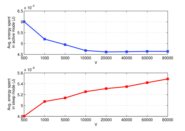
Figure 1: Avg. energy consumptions in active and sleep modes

Next, we conduct a simulation experiment to observe the bursty departure property of ESS algorithm explained in Lemma 1. As stated in Lemma 1, the nodes transmit their packets consecutively in order to reduce the switching energy. Figure 2 depicts the average number of bursty active staying which is the number of two or more consecutive time slots where the node is selected to be the active node and transmits. Higher values of $V$ push the nodes spend the minimum energy and in order not to consume switching energy the nodes are selected as the active node in a bursty fashion.

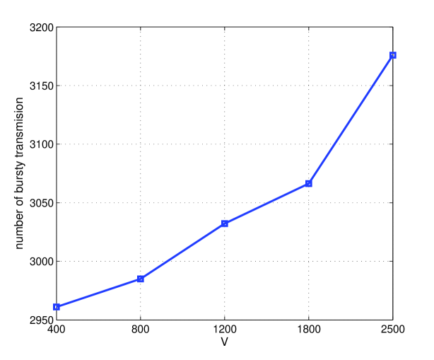
Figure 2: Bursty transmission

Furthermore, we compare the ESS algorithm with a “benchmark algorithm” and the S-MAC type algorithm proposed in [22] ,namely “periodic algorithm”, in terms of the average queue backlogs for different values of $V=400,800,1200,1800,2500$. Contrary to ESS, the benchmark algorithm ignores the switching energy and makes the switching and scheduling decisions without considering switching energy cost. Therefore, the nodes change their modes more frequently. In S-MAC type periodic algorithm, the nodes stay in sleep mode during the fist 1 ms and during the last 1 ms, they stay in active mode. Furthermore, the node which maximizes $Q_{n}(t)\mu_{n}(t)-V\alpha\mu_{n}(t)$ is selected as the transmitting node during the active period. As it is seen in Figure 3, the benchmark algorithm outperforms ESS in terms of the queue backlogs, since it stays in the active mode at most of the time.

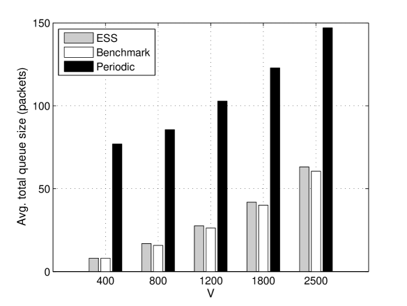
Figure 3: The average queue backlogs for different values of V

On the other hand, since ESS promotes the nodes to stay in sleep mode considering the switching cost, it prolongs the network lifetime. The periodic algorithm has the worst performance since it has fixed duty cycle property which can not ensure the efficient time to reduce the queue backlogs as much as ESS algorithm. Figure 4 depicts the comparison of the lifetime performance induced by ESS, the benchmark, the distributed and the periodic algorithms. The distributed algorithm allows more than one nodes to be active at any time slot and the benchmark algorithm does not care the switching energy cost. In addition, the periodic algorithm forces the nodes to be active for 1 ms at every slot and due tot he fixed duty cycle, $V$ does not effect the lifetime of periodic algorithm. Thus, with these algorithms, the nodes stays in active mode unnecessarily. As a result, batteries of the node run out quickly. Therefore, EES shows better performance result in terms of lifetime.

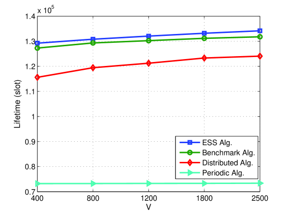
Figure 4: The network lifetime for different values of V

Finally, Figure 5 depicts the average duty cycle of the network per node. As $V$ increases, the proportion of time the nodes stay in active mode decreases to prevent the energy consumption. Thus, the average duty cycle period decreases as well. It is easy to see that the duty cycle per node can be approximately at most %13. As stated in [2], the switching energy needs to be computed if the node duty cycle is low. Thus, the effect of switching energy becomes significant.

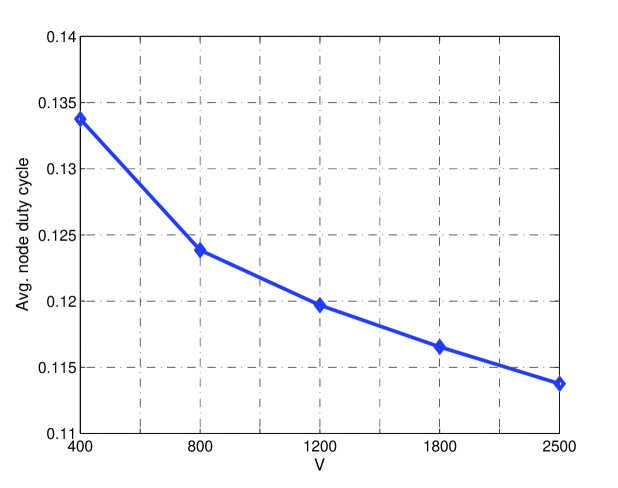
Figure 5: Duty cycle

VII Conclusion

In this paper, we investigate the energy efficiency and optimal control problems in a low duty cycle wireless sensor network. Using Lyapunov optimization technique, an energy-aware switching and scheduling (ESS) algorithm is proposed. The switching energy is generally not considered in energy management problems. However, analysis indicate that ESS algorithm outperforms the benchmark algorithm which ignores the switching energy cost in terms of the lifetime. Furthermore, we show that we can stabilize the network by applying ESS algorithm and push its performance to the optimal solution by tuning $V$ parameter. In addition, we present a distributed algorithm that can be implemented easily.

In terms of future work, we investigate the power control problem. Shortly, the power control problem is explained as follows. If the sensor nodes have power control, there is an inherent trade-off between the transmission power and the time spent in active mode. Note that the transmission rate $\mu_{n}(t)=\log\left(1+\frac{P_{n}(t)}{N}\right)$, where $P_{n}(t)$ and $N$ are the transmission and ambient noise powers respectively, is an increasing concave function. Therefore, as transmission power of node $n$ increases, the number of bits sent increases and the backlog of the active node drops below the aforementioned threshold more quickly.

References

- [1] I. Akiyldiz, W. Su, Y. Sankarasubramaniam, and E. Cayirci, “A survey on sensor networks, IEEE Com. Mag., vol. 40, no. 8, pp. 102 114, 2002.
- [2] A.G. Ruzzelli, P. Cotan, G.M.P O Hare, R. Tynan and P.J.M. Havinga, “Protocol Assessment Issues in Low Duty Cycle Sensor Networks: The Switching Energy”, in Proceedings of the IEEE International Conference on Sensor Networks, Ubiquitous, and Trustworthy Computing (SUTC2006), pp. 136-143, 2006.
- [3] L. Tassiulas and A. Ephremides, “Stability properties of constrained queueing systems and scheduling policies for maximum throughput in multihop radio networks,” IEEE Transactions on Automatic Control, vol. 37, pp. 1936-1949, 1992.
- [4] L. Georgiadis, M.J. Neely, and L. Tassiulas, “Resource Allocation and Cross-Layer Control in Wireless Networks”, Foundations and Trends in Networking, 2006.
- [5] W. Ye, J. Heidemann, and D. Estrin, “Medium access control with coordinated adaptive sleeping for wireless sensor networks”, IEEE/ACM Transactions on Networking, vol. 3, pp. 493-506, 2004.
- [6] A. Ruzzelli, M. O Grady, G. O Hare, and R. Tynan, “An energy-efficient and low-latency routing protocol forwireless sensor networks”, in Proceeding of the Advanced Industrial Conference on Wireless Technologies SENET 2005, 2005.
- [7] T. V. Dam and K. Langendoen, “An adaptive energy efficient mac protocol for wireless sensor networks”, Proceedings of the 1st international conference on Embedded networked sensor systems, pp. 171-180, 2003.
- [8] Rajendran, Obrazka, and Garcia-Luna-Aceves, “Energyefficient, collision-free medium access control for wireless sensor netwoks” Conference on Embedded Networked Sensor System, pp. 181-192, 2003.
- [9] I. Akyildiz, W. Su, Y. Sankarasubramaniam, and E. Cayirci, “Wireless sensor networks: A survey”, Computer Networks, vol. 38, pp. 393-422, 2002.
- [10] V. Raghunathan, C. Schurgers, S. Park, and M. B. Srivastava, “Energy-aware wireless microsensor networks”, IEEE Signal Processing Magazine, pp. 40-50, 2002.
- [11] G. Lu, B. Krishnamachari, Cauligi, and S. Raghavendra, “An adaptive energy-efficient and low-latency mac for data gathering in sensor networks”, International workshop on Alghoritms for Wireless, Mobile, ad Hoc Sensor Networks (WMAN 04), pp. 224-231, 2004.
- [12] J.Polastre, J.Hill, and D.Culler, “Versatile low power media access for wireless sensor networks”, in proc. ACM Sensys, 2004.
- [13] L.Gu and J.A. Stankovic, “Radio-Triggered Wake-Up Capability for Sensor Networks”, in Proceedings of the 10th IEEE Real-Time and Embedded Technology and Applications Symposium, 2004.
- [14] R. Jurdak, A.G. Ruzzelli, G.M.P O Hare, “Radio Sleep Mode Optimization in Wireless Sensor Networks”, IEEE Transactions on Mobile Computing, vol. 9, no.7, 2010.
- [15] A.G. Ruzzelli, G.M.P O Hare and R.Jurdak, “MERLIN:Cross-Layer Integration of MAC and Routing for Low Duty-Cycle Sensor Networks”, Ad Hoc Networks journal, vol. 7, pp. 1238-1257, 2008.
- [16] J. Chang and L. Tassiulas, “Energy conserving routing in wireless ad hoc networks”, IEEE INFOCOM, 2000.
- [17] Avinash Sridharan, Scott Moeller and Bhaskar Krishnamachari “Making distributed rate control using Lyapunov drifts a reality in wireless sensor networks , 6th Intl. Symposium on Modeling and Optimization in Mobile, Ad Hoc, and Wireless Networks (WiOpt), pp. 452-461, 2008.
- [18] M. Gatzianas, L. Georgiadis and L. Tassiulas, “Control of wireless networks with rechargeable batteries”, IEEE Transactions on Wireless Communications, vol. 9, pp. 581-593, 2010.
- [19] Y. Song, C. Zang, Y. Fang and Z. Niu, “Energy-Conserving Scheduling in Multi-hop Wireless Networks with Time-Varying Channels”, IEEE INFOCOM, 2010.
- [20] M. J. Neely, “Energy Optimal Control for Time Varying Wireless Networks”, IEEE Transactions on Information Theory, vol. 52, pp. 2915-2934, 2006.
- [21] M. Cagalj, J. P. Hubaux and C. Enz, “Minimum-energy broadcast in all-wireless networks: NP-completeness and distribution issues”, Proceedings of the 8th annual international conference on Mobile computing and networking, pp. 172-182, 2002.
- [22] W. Ye, J. Heidemann, and D. Estrin, “Medium Access Control with Coordinated Adaptive Sleeping for Wireless Sensor Networks, IEEE/ACM Trans. Net., vol. 12, no. 3, June 2004, pp. 493 506.