Heat conductivity in the $\beta$-FPU lattice.
Solitons and breathers as energy carriers

Abstract

This paper consists of two parts. The first part proposes a new methodological framework within which the heat conductivity in 1D lattices can be studied. The total process of heat conductivity is decomposed into two contributions where the first one is the equilibrium process at equal temperatures $T$ of both lattice ends and the second – non-equilibrium process with the temperature $\Delta T$ of one end and zero temperature of the other. This approach allows to isolate and analyze the heat transfer in explicit form. The heat conductivity in the limit $\Delta T\to 0$ is reduced to the heat conductivity of harmonic lattice with stochastic rigidities determined by the equilibrium process at temperature $T$. A threshold temperature $T_{\rm thr}$ is found which separates two regimes: small perturbations exponentially decay at $T<T_{\rm thr}$ and tend to constant value at $T>T_{\rm thr}$. The threshold temperature scales $T_{\rm thr}(N)\sim N^{-3}$ with the lattice size $N$ and $T_{\rm thr}\to 0$ in the thermodynamic limit. Some unusual properties of heat conductivity can be exhibited on nanoscales at low temperatures. The thermodynamics of the $\beta$-FPU lattice can be adequately approximated by the harmonic lattice with temperature renormalized coefficients of rigidity. The second part testifies in the favor of the soliton and breather contribution to the heat conductivity in contrast to conclusions made in [N. Li, B. Li, S. Flach, PRL 105 (2010) 054102]. In the long-wavelength continuum limit the discrete $\beta$-FPU lattice is reduced to the modified Korteweg – de Vries equation. This equation has soliton and breather solutions. Numerical simulations demonstrate their high stability. New method for the visualization of moving solitons and breathers is suggested. An accurate expression for the dependence of the sound velocity on temperature is also obtained. Our results support the conjecture on the solitons and breathers contribution to the heat conductivity. The fraction of total heat flux transferred by solitons and breathers merits additional analysis.

Keywords: heat conductivity, $\beta$-FPU lattice, soliton, breather

^∗The corresponding author: gvin@deom.chph.ras.ru.

I Introduction

The problem of heat conductivity in low dimensional systems attracts much attention in last decades (see review Lep03 ) and is motivated by the discovery of quasi-one-dimensional (nanotubes, nanowires, etc.) and two-dimensional (graphen, graphan, etc.) systems.

The modern theory of heat conductivity was initiated by the celebrated preprint of E. Fermi, J. Pasta, and S. Ulam Fer55 , though the primary aim was “of establishing, experimentally, the rate of approaching to the equipartition of energy among the various degrees of freedom”. Subsequent investigations demonstrated wide area of consequences in many physical and mathematical phenomena (see reviews in special issues of journals CHAOS Cha05 and Lecture Notes in Physics Lec08 devoted to the 50th anniversary of the FPU preprint).

The dynamical properties of nonlinear systems in microcanonical ensemble (total energy $E=$ const) were thoroughly analyzed. It allows to investigate the dynamics and to get exact results (soliton Kru64 ; Zab65 ; Dod82 and breather Cam96 ; Sie88 ; Dau93 ; Aub94 ; Mac94 solutions), to analyze regular and stochastic regimes and to find the corresponding thresholds. The FPU preprint also initiated the investigations in the field of “experimental mathematics” Por09 .

About ten decades ago P. Debye argued that the nonlinearity can be responsible for the finite value of heat conductivity in insulating materials Deb14 . But modern analysis shows that it is not always the case. There are many examples where the coefficient of heat conductivity $\varkappa$ diverges with the increasing system size $L$ as $\varkappa\propto L^{\alpha}$ where $\alpha>0$, and $\varkappa\to\infty$ in the thermodynamic limit ($L\to\infty$). Most of momentum conserving one-dimensional nonlinear lattices with various types of nearest-neighbor interactions have this unusual property (see, e.g., Lep03 ; Cas05 ; Lic08  ). Moreover, some other systems, – two- Bar07 ; Lip00 ; Sai10 and three-dimensional lattices Shi08 , polyethylene chain Hen09 , carbon nanotubes Yao05 ; Yu_05 ; Mar02 ; Min05 ; Cao04 have analogous property – diverging heat conductivity with the increasing size of the system.

There were some conjectures explaining the anomalous heat conductivity. Generally speaking, whenever the equilibrium dynamics of a lattice can be decomposed into that of independent “modes” or quasi-particles, the system is expected to behave as an ideal thermal conductor Lep05 . Thereby, the existence of stable nonlinear excitations is expected to yield ballistic rather than diffusive transport. At low temperatures normal modes are phonons. At higher temperatures noninteracting “gas” of solitons or/and breathers starts to play more significant role, and M. Toda was the first who suggested the possibility of heat transport by solitons Tod79 .

Though analytical expressions for solitons can be derived only for few continuum models described by partial differential equations, Friesecke and Pego in a series of recent papers Fri99 ; Fri02 ; Fri04a ; Fri04b made a detailed study of the existence and stability of solitary wave solutions on discrete lattices with the Hamiltonian $H=\sum_{i}\frac{1}{2}p_{i}^{2}+u(y_{i})$, where $y_{i}=x_{i}-x_{i-1};\ p_{i}=\dot{x}_{i}$. It has been proven that the systems with this Hamiltonian and with the following generic properties of nearest-neighbor interactions: $u^{\prime}(0)=0;\ u^{\prime\prime}(0)>0;\ u^{\prime\prime\prime}(0)\neq 0$ has a family of solitary wave solutions which in the small amplitude, long-wavelength limit have a profile close to that of the KdV soliton. It was also shown Hof08 that these solutions are asymptotically stable. Thus most acceptable point of view on the origin of anomalous heat conductivity in nonlinear lattices is as follows: phonons are responsible for heat conductivity at low temperatures, and at high temperatures – solitons Li_05 ; Vil02 .

Rather confusing experimental and numerical results are demonstrated in literature about the dependence of heat conductivity on different parameters, – model under consideration, types of boundary conditions, used thermostat and temperature. For instance, temperature dependence of heat conductivity in carbon nanotubes decreases as $\varkappa\sim 1/T$ at $T>10$ K Mar03 ; experimentally is found Yu_05 that $\varkappa$ also decreases with the growth of temperature. Different temperature dependencies $\varkappa$ vs. $T$ were found in 1D nonlinear lattices. For $\beta$-FPU lattice: $\varkappa\sim N^{\alpha}T^{-1}$ at $T\lesssim 0.1$ and $\varkappa\sim N^{\alpha}T^{1/4}$ at $T>50$ Aok01 what is usually observed in insulating crystals. For the interparticle harmonic potentials and on-site potentials (e.g. Klein-Gordon chains) $\varkappa\sim T^{-1.35}$, i.e. heat conductivity decreases with the growth of temperature Aok00 . But there exists firm theoretical background Nar02 that the exponent $\alpha$ in the dependence $\varkappa\propto N^{\alpha}$ is the universal constant $\alpha\approx 1/3$ in momentum-conserving systems.

The calculation of heat conductivity at small temperature gradients is an additional problem. Usually these calculations are very time consuming because of great fluctuations of heat current and statistical averaging over large number of MD trajectories is necessary.

The paper organized as follows. In section II the heat conductivity is considered when the temperature gradient $\nabla T$ is small. The explicit contribution to the heat conductivity is extracted by the decomposing of the total process into two parts. The first one is the equilibrium process at temperatures $T$ of both lattice ends, and the second – non-equilibrium, when one lattice end has temperature $\Delta T$ and the other – zero temperature. Namely the latter process is responsible for the heat conductivity. This method allows to find the threshold temperature $T_{\rm thr}$. And though $T_{\rm thr}$ scales with the lattice length $N$ as $T_{\rm thr}\sim N^{-3}$, unusual dynamics can be revealed on nanoscale when both $T$ and $N$ are small. The low temperature thermodynamics can be adequately described in terms of harmonic lattice with temperature renormalized rigidity coefficients.

Section III is independent of the previous one and is aimed at elucidating the role of solitons and breathers in the heat conductivity. Solitons and breathers are found as the solutions of the modified Korteweg – de Vries equation. This equation is obtained in the continuum limit from the discrete $\beta$-FPU lattice. Soliton and breather solution are checked in numerical simulation and demonstrate very high stability.

Necessary details of the derivation of accurate soliton and breather solutions in the continuum limit are given in Appendix.

II Heat conductivity in the $\beta$-FPU lattice

We consider the one-dimensional $\beta$-FPU lattice of $N$ oscillators with the interaction of nearest neighbors

$$U=\sum\limits_{i}\dfrac{\alpha}{2}(x_{i}-x_{i-1})^{2}+\dfrac{\beta}{4}(x_{i}-x_{i-1})^{4}$$ (1)

(usually the dimensionless potential will be used below, that is $\alpha=\beta=m=1$). Nonequilibrium conditions are necessary for the heat transport simulation. The most abundant method is the placement of the lattice into the heat bath with different temperatures of left $T_{+}$ and right $T_{-}$ ends ($T_{+}>T_{-}$). Different types of heat reservoirs are thoroughly analyzed in Lep03 . The usage of the Langevin forces with the noise terms and friction forces acting on the left $F_{+}=\xi_{+}-\gamma\dot{x}_{1}$ and right $F_{-}=\xi_{-}\gamma\dot{x}_{N}$ oscillators is the common practice ($\gamma=1$ is also put for brevity). $\left\{\xi_{\pm}\right\}$ are independent Wiener processes with zero mean and the correlator $\left<\xi_{\pm}(t_{1})\,\xi_{\pm}(t_{2})\right>=2T_{\pm}\,\delta(t_{1}-t_{2})$. $\Delta T=(T_{+}-T_{-})$ is the temperature difference. The generalized Langevin dynamics with a memory kernel and colored noises is also suggested Wan07 to correctly account for the effect of the heat baths.

The following set of stochastic differential equations (SDEs)

$$\ddot{x}_{i}=-\dfrac{\partial U}{\partial x_{i}}+\delta_{i1}F_{+}+\delta_{iN}F_{-}$$ (2)

is usually solved to find the heat flux $J$. And the local heat flux (power transmitted from $i$th to $(i+1)$th oscillator) is Zha02

$$J_{i\to i+1}=F_{i\to i+1}\,\dot{x}_{i+1};\qquad F_{i\to i+1}\equiv-U^{\prime}(x_{i+1}-x_{i}),$$ (3)

where $F_{i\to i+1}$ is a shorthand notation for the force exerted by the $i$th on the $(i+1)$th oscillator. The total heat flux $J$ can be found as the mean $J=(N-1)^{-1}\sum_{i}^{N-1}J_{i\to i+1}$.

II.1 Equilibrium and non-equilibrium contributions to the heat conductivity

If $T_{-}\neq 0$ then the process of heat conductivity can be formally decomposed into two contributions: the first one – equilibrium process with equal temperatures $T_{-}$ of both lattice ends; and the second – nonequilibrium process with temperature $\Delta T$ of the left lattice end and zero temperature of the right end (see Fig. 1) (by ‘process’ we hereafter assume for brevity the solution ${\bf x}(t)=\left\{x_{1}(t),x_{2}(t),\ldots,x_{N}(t)\right\};\,{\bf v}(t)=\left\{v_{1}(t),v_{2}(t),\ldots,v_{N}(t)\right\}$ of the corresponding SDEs).

Figure 1: Schematic representation of the total process ${\bf x}(t)$ as sum of equilibrium ${\bf x}^{0}(t)$ and non-equilibrium ${\bf x}^{1}(t)$ processes.

Namely the second process is responsible for the heat transport taking place on(?) the background of equilibrium process. Once this approach is utilized then the noise terms in (2), owing to their independence, are $\left\{\xi_{+}\right\}=\left\{\xi^{0}\right\}+\left\{\xi^{1}\right\}$ and $\left\{\xi_{-}\right\}=\left\{\xi^{0}\right\}$ for the left and right lattice ends, correspondingly Superscripts ‘0’ and ‘1’ refer to equilibrium and nonequilibrium processes. The total process ${\bf x}(t)$ can be represented as the sum

$${\bf x}(t)={\bf x}^{0}(t)+{\bf x}^{1}(t),$$ (4)

where ${\bf x}^{0}(t)$ is the equilibrium (Gibbs’s) process at temperature $T_{-}$, and ${\bf x}^{1}(t)$ – nonequilibrium, responsible for the energy transport, process. The corresponding stochastic dynamics is

$$\ddot{x}_{i}^{0}=-\dfrac{\partial U^{0}}{\partial x_{i}^{0}}+\delta_{i1}(\xi^{0}-\dot{x}^{0}_{1})+\delta_{iN}(\xi^{0}-\dot{x}^{0}_{N}),$$ (5)

$$\ddot{x}_{i}^{1}=-\left[\dfrac{\partial U}{\partial x_{i}}-\dfrac{\partial U^{0}}{\partial x_{i}^{0}}\right]+\delta_{i1}(\xi^{1}-\dot{x}^{1}_{1})+\delta_{iN}(-\dot{x}^{1}_{N}),$$ (6)

and the sum of equations (5) and (6) is identical to the parent equation (2). Random values $\left\{\xi^{0}\right\}$ and $\left\{\xi^{1}\right\}$ obey the identities $\left<\xi^{0}(t_{1})\xi^{0}(t_{1})\right>=2T_{-}\delta(t_{1}-t_{2})$ and $\left<\xi^{1}(t_{1})\xi^{1}(t_{1})\right>=2\,\Delta T\delta(t_{1}-t_{2})$; $U^{0}$ is the total energy (1) where the arguments $x_{1}(t),x_{2}(t),\ldots,x_{N}(t)$ of the total process are replaced by coordinates of the equilibrium process $x_{1}^{0}(t),x_{2}^{0}(t),\ldots,x_{N}^{0}(t)$. Expression in the square brackets in (6) is the difference of forces acting on the $i$th oscillator from the total process ${\bf x}(t)$ and equilibrium process ${\bf x}^{0}(t)$. It is worth mentioning that this force is the random value, and the process ${\bf x}^{1}(t)$ (heat transport) is realized in the lattice with time-dependent random potentials. The problem of heat conductivity in the random time-independent potentials was analyzed in Joh08 .

Equation (5) describes the system embedded in the heat reservoir at temperature $T_{-}$ of both lattice ends. And ${\bf x}^{0}(t)$ is the stationary equilibrium process described by the canonical Gibbs distribution. Process ${\bf x}^{1}(t)$ is responsible for the heat transport and the Wiener process $\left\{\xi^{1}(t)\right\}$ on the left lattice end defines temperature $\Delta T$. Right lattice end has zero temperature (only the friction force acts on this oscillator). An expression for the local heat flux is

$$J_{i\to i+1}=\left[F_{i\to i+1}({\bf x})-F_{i\to i+1}({\bf x}^{0})\right]\,\dot{x}_{i+1}^{0},$$ (7)

and the equilibrium process ${\bf x}^{0}$ does not transfer energy: $\left<F_{i\to i+1}({\bf x}^{0})\,\dot{x}^{0}_{i+1}\right>\equiv 0$, where $\left<\ldots\right>$ stands for the time average. It is essential that the heat flux (7) is the small difference of large values from processes ${\bf x}(t)$ and ${\bf x}^{0}(t)$. This is the reason why MD simulation gives large fluctuation when $\Delta T\to 0$ and $T$ is not low. It can be shown that the time of computation increases $\propto(\Delta T)^{-2}$ if the standard error is fixed. The comparison of two approaches (solving of standard SDEs (2) and (5)-(6)) is shown in Fig. 2 and results coincide with very good accuracy.

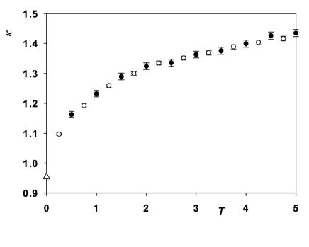
Figure 2: Temperature dependence of heat conductivity for the lattice of $N=5$ oscillators. Filled circles: solution of standard SDEs (2); empty circles: SDEs (5)-(6). Averaging over $100$ MD trajectories $10^{4}$ time units (t.u.) each. $T_{-}=0{.}2$, $\Delta T=0{.}01T_{-}$. Triangle up at $T=0$ is the exact value in the harmonic approximation ($\beta=0$).

Some results in this paper are obtained for the number of oscillators $N=5$. It may appear that this value is too small. For instance, “standard” simulations require up to $\sim 10^{4}$ particles and $\sim 10^{8}$ integration steps plus ensemble averaging Lep03 . But our results are aimed at establishing some new issues where number of particles is unessential. Lattices with larger number of oscillators were tested when necessary.

Relative displacements $(x_{i}^{0}-x_{i-1}^{0})$ and $(x_{i}^{1}-x_{i-1}^{1})$ for processes ${\bf x}^{0}(t)$ and ${\bf x}^{1}(t)$ are shown in Fig. 3. These values characterize the energy fluxes in the lattice. Energy fluxes to the left and to the right are equal on average for process ${\bf x}^{0}(t)$ as it is the equilibrium process without energy transfer. But the energy flux is directed mainly to the right for process ${\bf x}^{1}(t)$ (right panel). Low temperature is chosen for the better illustration.

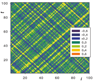
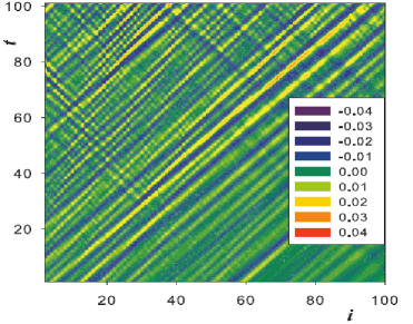
Figure 3: Spatiotemporal evolutions of relative displacements $(x_{i}^{0}-x_{i-1}^{0})$ and $(x_{i}^{1}-x_{i-1}^{1})$ for the equilibrium ${\bf x}^{0}(t)$ (left panel) and nonequilibrium ${\bf x}^{1}(t)$ (right panel) processes. $N=100$, $T_{-}=0{.}05$, $\Delta T=0{.}0001$.

The dependence of heat conductivity on the oscillators number $N$ is shown in Fig. 4 at two value of temperature $T_{-}$. Results coincide with very good accuracy. Inharmonicity becomes negligible at low temperature and heat conductivity at $T_{-}=0{.}1$ (cirles in Fig. 4) coincides with the heat conductivity of the harmonic lattice (dashed line) with good accuracy. The analytical solution of the heat conductivity for the harmonic lattice is given in Rie67 .

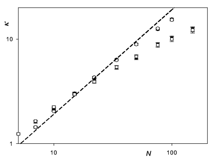
Figure 4: Coefficient of heat conductivity for the $\beta$-FPU lattice for $N=7-150$ oscillators. Squares: $T_{-}=1$, circles: $T_{-}=0{.}1$. Filled symbols – results obtained by the solution of standard SDEs (2), empty symbols – SDEs (5)-(6). Averaging over 200 MD trajectories $3\,10^{4}$ t.u. $\Delta T=0{.}01T_{-}$. Dashed line – harmonic approximation. Filled symbols are practically fully covered by empty symbols and are invisible.

There should be solved twice as large SDEs (5)-(6) in suggested approach as that in standard scheme (2). But this approach has some undoubted merits as discussed below.

II.2 Heat conductivity at small temperature gradients

One of the goals of the present paper is the computation of heat conductivity at very small temperature gradients. With this in mind an expression for the heat flux is analyzed in more details. The expression for the local heat flux (7) can be rewritten as

$$\begin{split}J_{i\to i+1}=&\left[F_{i\to i+1}({\bf x})-F_{i\to i+1}({\bf x}^{0})\right]\dot{x}_{i+1}^{1}=\\ {}&\left[-(x_{i+1}-x_{i})-(x_{i+1}-x_{i})^{3}+(x^{0}_{i+1}-x^{0}_{i})+(x^{0}_{i+1}-x^{0}_{i})^{3}\right]\dot{x}_{i+1}^{1},\end{split}$$ (8)

where $\dot{x}_{i+1}^{1}$ – velocity of $(i+1)$th oscillator in process ${\bf x}^{1}$. Taking in mind that $x_{i}=x_{i}^{0}+x_{i}^{1}$, the expression (8) can be transformed to

$$J_{i\to i+1}=\left\{-(x_{i+1}^{1}-x_{i}^{1})\left[1+3\,(x_{i+1}^{0}-x_{i}^{0})^{2}\right]+(x_{i+1}^{1}-x_{i}^{1})^{2}\left[1+3\,(x_{i+1}^{0}-x_{i}^{0})\right]\right\}\dot{x}_{i+1}^{1}.$$ (9)

Processes ${\bf x}^{0}(t)$ and ${\bf x}^{1}(t)$ have different ranges of specific energies. Noise terms $\left\{\xi^{1}\right\}$, which provide temperature $\Delta T$, are of the order $\xi^{1}\sim\sqrt{\Delta T}$ (as $\left<\xi^{1}(t_{1})\xi^{1}(t_{2})\right>\sim\Delta T$). And one can expect that process ${\bf x}^{1}(t)$ has the same order ${\bf x}^{1}(t)\sim\sqrt{\Delta T}$ because equations (6) become linear in the limit $\Delta T\to 0$ when $\xi^{1}\to 0$. Expression in curly brackets in (9) is the polynomial of the third degree in the square root of temperature difference $\sqrt{\Delta T}$. Taking into account that the velocity $\dot{x}_{i+1}^{1}$ is also of the order $\sim\sqrt{\Delta T}$, expression (9) is the polynomial of the forth degree in $\sqrt{\Delta T}$. But the coefficient of heat conductivity is determined by the relation $J/\Delta T$. Then terms of the third and forth orders can be neglected at $\Delta T\to 0$. Then (9) is simplified to

$$J_{i\to i+1}=-\left(x_{i+1}^{1}-x_{i}^{1}\right)\left[1+3\,\left(x_{i+1}^{0}-x_{i}^{0}\right)^{2}\right]\dot{x}_{i+1}^{1}.$$ (10)

An expression for the potential energy, corresponding to process ${\bf x}^{1}(t)$, can be derived analogously. This energy is the difference of potential energies $U({\bf x})-U^{0}({\bf x}^{0})$ and again, using coordinates ${\bf x}$ and ${\bf x}^{0}$, and preserving only terms quadratic in $(x_{i+1}^{1}-x_{i}^{1})$, one can get the potential energy for process ${\bf x}^{1}$ in the form

$$U^{1}=\dfrac{1}{2}\sum_{i}g_{i+1}(t)\,(x_{i+1}^{1}-x_{i}^{1})^{2},\qquad g_{i+1}(t)=1+3\,[x_{i+1}^{0}(t)-x_{i}^{0}(t)]^{2}\,,$$ (11)

where $g_{i}(t)$ are time-dependent random coefficients of rigidities determined by process ${\bf x}^{0}(t)$.

It is illuminating to note that in the limit $\Delta T\to 0$ the problem of heat conductivity in the $\beta$-FPU lattice is reduced to the harmonic lattice with random coefficients. Corresponding SDEs have noise terms with friction forces on the left oscillator and zero temperature (only viscous forces) on the right oscillator:

$$\ddot{x}_{i}^{1}=-g_{i}(x_{i}^{1}-x_{i-1}^{1})+g_{i+1}(x_{i+1}^{1}-x_{i}^{1})+\delta_{i1}(\xi^{1}-\dot{x}_{1}^{1})-\delta_{iN}\dot{x}_{N}^{1}$$ (12)

and $g_{i},g_{i+1}$ are defined in (11). If the 1D lattice with an arbitrary interaction potential is analyzed then the corresponding equations are the same with rigidities $g_{i}=U^{\prime\prime}(x^{0}_{i}-x^{0}_{i-1}$) where $U$ is the potential energy. SDE for the system with arbitrary neighbor radius of interaction can be written in the general form as

$$\ddot{x}_{i}^{1}=-\sum_{j=1}^{M}{\bf\Lambda}_{ij}^{0}\,x_{j}^{1}+\delta_{i1}(\xi^{1}-\dot{x}_{1}^{1})-\delta_{iN}\dot{x}_{N}^{1}\,,$$ (13)

where ${\bf\Lambda}_{ij}^{0}$ – matrix of second derivatives of potential energy depending on ${\bf x}^{0}$, and $M$ is the number of neighbors.

II.3 Unusual dynamics of process ${\bf x}^{1}(t)$ at high temperatures

The process ${\bf x}^{1}(t)$ can be characterized by some time average correlators. The correlator $\left<\left[x_{1}^{1}(t)\right]^{2}\right>$ was analyzed for the better understanding of the dynamics of process ${\bf x}^{1}(t)$. One can expect that $\left<\left[x_{1}^{1}(t)\right]^{2}\right>\sim\Delta T$ as discussed above. Two temperatures of the background process $T_{-}$ were tested: $T_{1}=0{.}2$ and $T_{2}=5$ (hereafter subindex ‘–’ is omitted, that is $T_{-}=T$). Results are shown in Fig. 5.

As expected, the correlator $\left<\,[x_{1}^{1}(t)]^{2}\right>$ linearly depends on $\Delta T$: $\left<\,[x_{1}^{1}(t)]^{2}\right>\sim\Delta T$ at $T_{1}=0{.}2$. But the case is quite different at $T_{2}=5$: $\left<\,[x_{1}^{1}(t)]^{2}\right>$ reaches the stationary value $\approx 0{.}064$ in the limit $\Delta T\to 0$. It means that there exists some undamped stationary process ${\bf x}^{1}(t)$ at high temperatures $T$ of the background process ${\bf x}^{0}(t)$ even in the limit $\Delta T\to 0$. These results also imply an existence of a threshold temperature $T_{\rm thr}$ separating two regimes – damped at low temperatures and undamped at high temperatures.

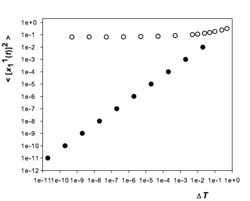
Figure 5: Dependence of correlator $\left<(x_{1}^{1})^{2}\right>$ on the temperature difference $\Delta T$. Filled circles: $T=0{.}2$, empty circles: $T=5$. Asymptotic value $\left<(x_{1}^{1})^{2}\right>_{\Delta T\to 0}\approx 0{.}064$ at $T=5$ (coefficient of linear regression $0{.}9993$). Averaging over 100 MD trajectories $10^{4}$ t.u. each. $N=5$. The range of $\Delta T$: $10^{-11}\leq\Delta T/T\leq 2\!\cdot\!10^{-1}$.

II.4 Threshold temperature

Any process ${\bf x}^{1}(t)$ damps out at low temperatures and flattens out to a stationary value at higher temperatures even in the limit $\Delta T\to 0$, and the temperature $T$ of process ${\bf x}^{0}(t)$ defines different damping rates. Bearing this in mind, it is convenient to excite some auxiliary process $\widetilde{\bf x}^{1}(t)$ over the background process ${\bf x}^{0}(t)$ and to analyze it.

Coordinates and velocities of process $\widetilde{\bf x}^{1}(t)$ get random increments $\frac{1}{2}\sum_{i}[{\widetilde{x}}_{i}^{1}(t=0)]^{2}+\frac{1}{2}\sum_{i}[{\widetilde{v}}_{i}^{1}(t=0)]^{2}=0{.}5$. The particular choice of initial conditions does not influence the final results. The total dynamics is the sum of two processes ${\bf x}(t)={\bf x}^{0}(t)+\widetilde{\bf x}^{1}(t)$.

Stochastic differential equations for the process ${\bf\widetilde{x}}^{1}(t)$ are

$$\ddot{\widetilde{x}}_{i}^{1}=-\left[\dfrac{\partial U}{\partial x_{i}}-\dfrac{\partial U^{0}}{\partial x_{i}^{0}}\right]-\delta_{i1}\dot{\widetilde{x}}^{1}_{1}-\delta_{iN}\dot{\widetilde{x}}^{1}_{N}$$ (14)

and only viscous forces acts at the extreme left and right oscillators. $U$ and $U^{0}$ are potential energies with coordinates ${\bf x}(t)$ and ${\bf x}^{0}(t)$, correspondingly. Stochastic dynamics (14) is implicitly ruled out by the temperature $T$ of process ${\bf x}^{0}(t)$.

To find the threshold temperature we initially consider the case of small temperature $T$ when process ${\bf\widetilde{x}}^{1}(t)$ is damped out. Its damping is determined by the viscous friction of left $(-\dot{\widetilde{x}}^{1}_{1})$ and right $(-\dot{\widetilde{x}}^{1}_{N})$ oscillators in (14). Gradually increasing the temperature its threshold value can be found when process ${\bf\widetilde{x}}^{1}(t)$ becomes undamped. The damping of mean squared displacement of the first oscillator $[{\widetilde{x}}_{1}^{1}(t)]^{2}$ was calculated. Process $\widetilde{\bf x}^{1}(t)$ exponentially decays $\left<\,[\widetilde{x}_{1}^{1}(t)]^{2}\right>\propto\exp(-\alpha t)$ and $\alpha$ depends on $T$ (see Fig. 6a).

!

!

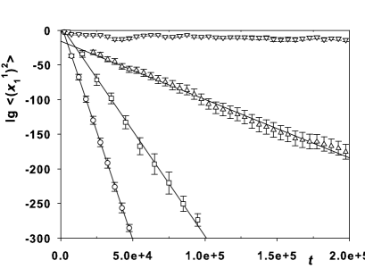
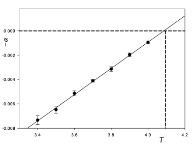
Figure 6: a) Exponential damping of process ${\bf\widetilde{x}}^{1}(t)$ at different temperatures: $T=3{.}5$ (circles), $T=3{.}8$ (squares), $T=4{.}0$ (triangles up), $T=4{.}2$ (triangles down). Solid lines – linear regressions. Averaging time $\sim\!5\,000-10\,000$ t.u. 20 trajectories ${\bf x}^{0}$ were used to estimate the standard error. b) Damping coefficient $(-\alpha)$ as the function of temperature $T$ of process ${\bf x}^{0}(t)$. Damping stops $(\alpha=0)$ at $T_{\rm thr}\simeq 4{.}07$. $N=5$.

The temperature dependence of coefficient $\alpha$ is shown in Fig. 6b and $T_{\rm thr}\simeq 4{.}07$ when $\alpha=0$.

Next method to find the threshold temperature is moving “from up to down”, going from higher to lower temperatures. At high temperatures there exists the stationary process arising from random forces $\Phi_{i}=\left[{\partial U}/{\partial x_{i}}-{\partial U^{0}}/{\partial x_{i}^{0}}\right]$ (see (14)). And process ${\bf\widetilde{x}}^{1}(t)$ decreases in a sense that all quadratic mean values tend to zero as temperatures approaches $T_{\rm thr}$ from above. When the temperature reaches its threshold value, process ${\bf\tilde{x}}^{1}(t)$ is totally damped (see Fig. 7). The found threshold temperature is $T_{\rm thr}\simeq 4{.}09$.

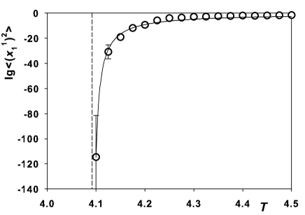
Figure 7: Stationary values $\left<(\widetilde{x}_{1}^{1})^{2}\right>$ at $T>T_{\rm thr}$. Time of averaging $~{}10^{6}$ t.u. The temperature dependence is approximated by the function $\left<[\widetilde{x}_{1}^{1}(t)]^{2}\right>\sim\exp[-b/(T-T_{\rm thr})]$ (solid line). $N=5$.

Strange behavior of process ${\bf x}^{1}(t)$ is basically explained by time-dependent random forces $\Phi_{i}=\left[{\partial U}/{\partial x_{i}}-{\partial U^{0}}/{\partial x_{i}^{0}}\right]$ (see (6)) rather then random Langevin forces $\xi^{1}\sim\sqrt{\Delta T}$. And the plateau for the correlator $\left<[x^{1}_{1}(t)]^{2}\right>\approx 0{.}064$ at $\Delta T\to 0$ is determined exclusively by the background process ${\bf x}^{0}$.

This conjecture can be additionally supported. Let us consider the case of low temperatures $T$ when process ${\bf x}^{0}$ is “weak”. Then the rigidity coefficients $g_{i}$ in (11) are close to unity. The lattice where actual rigidity coefficients $g_{i}$ (11) are substituted by the mean values taken from the equilibrium Gibbs distribution: $\left<g_{i}\right>=g_{0}(T)$ and $g_{0}(T)=1+3\left<(x^{0}_{i}-x^{0}_{i-1})^{2}\right>$ is considered as an example. This harmonic model is exactly solvable and results are shown in Fig. 8

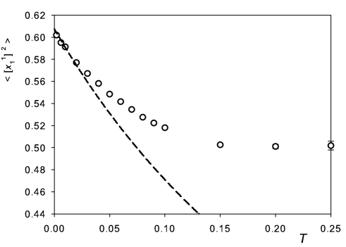
Figure 8: Temperature dependence of the mean squared displacement $\left<[x_{1}(t)]^{2}\right>$. Circles – MD simulation of SDEs (12); dashed line – model of mean rigidities in the harmonic approximation. Averaging over 20 trajectories $2\,10^{4}$ t.u. each.

One can see that process $\left<[x_{1}^{1}(t)]^{2}\right>$ damps out in the model with constant rigidity in contrast to the case when actual values (11) are used. And the growth of process $\left<[x_{1}^{1}(t)]^{2}\right>$, when temperature increases, is mainly governed by fluctuations rather then the increasing rigidities.

Additional evidence of threshold phenomena is the one-dimensional analogue of the Mathieu equation

$$\ddot{x}=-[1+g\cos^{2}(t)]\,x.$$ (15)

Different types of solutions depend on the parameter $g$ and initial conditions. There exists such critical value $g_{\rm cr}$ that the solution is the superposition of periodic functions at $g<g_{\rm cr}$, and the solution diverges $\propto\exp(\pm\mu t)$ at $g>g_{\rm cr}$.

We consider an equation for the harmonic oscillator for one variable $x$ with friction force

$$\ddot{x}=-k(t)x-\dot{x},$$ (16)

where $k(t)$ – stochastic rigidity. This equation is similar to equation (12) for process ${\bf x}^{1}(t)$ if $k(t)=1+3z^{2}(t)$ and $z(t)$ is the stochastic process generated by the dynamics of harmonic oscillator with noise term and friction force at temperature $T$:

$$\ddot{z}=-z+\xi-\dot{z}$$ (17)

and spectral property $\left<\xi(t_{1})\,\xi(t_{2})\right>=2T\delta(t_{1}-t_{2})$. The substitution $x\exp(-t/2)\to X$ excludes damping and (16) becomes

$$\ddot{X}=-[1+3z^{2}(t)]X,$$ (18)

what is similar to the Mathieu’s equation (15).

Eqs. (17)-(18) have rich family of solutions depending on initial conditions, temperature $T$ and the sequence $\left\{{\bf\xi}\right\}$. The solution is nearly harmonic function at very low temperatures. The superposition of harmonic functions is the solution at higher temperatures. At last there exists such threshold temperature $T_{\rm thr}$ that the solution diverges and is the product of harmonic functions by $\exp(\mu t)$. The solution is the product of some stochastic process by $\exp(\nu t)$ at much higher temperatures, and $\nu>\mu$. There are many interesting intermediate solutions, and this problem merits more attention. Considered examples show that an existence of threshold phenomena is not exceptional and can occur in different dynamical systems.

The threshold temperature $T_{\rm thr}\approx 4{.}1$ was found for the lattice length $N=5$. Larger lattice lengths were considered and the dependence of $T_{\rm thr}$ on the lattice length $N$ is shown in Fig. 9. Fitting gives dependence $T_{\rm thr}\approx 6\cdot 10^{2}\,N^{-3}$.

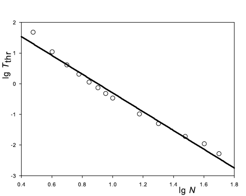
Figure 9: Dependence of $T_{\rm thr}$ vs. lattice length $N$ in log-log coordinates. Solid line is the fitting $T_{\rm thr}\sim N^{-3}$.

II.5 Time-resolved dynamics of process ${\widetilde{\bf x}}^{1}(t)$

Dynamics of process ${\widetilde{\bf x}}^{1}(t)$ at high temperatures $T$ was analyzed above in terms of time-average correlators. And time-resolved behavior of process ${\widetilde{\bf x}}^{1}(t)$ at two temperatures $T$ of the background process ${\bf x}^{0}$ is shown in Fig. 10. As above, ${\Delta}(t)=[\widetilde{x}_{1}^{1}(t)]^{2}$ was calculated.

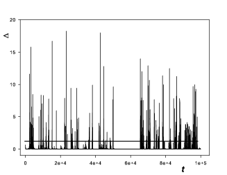
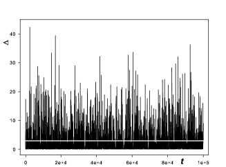
Figure 10: Dependence of ${\Delta}(t)=[\widetilde{x}_{1}^{1}(t)]^{2}$ on time at different temperatures of process ${\bf x}^{0}(t)$. Left panel: $T=4{.}3$; right panel: $T=7{.}0$. $N=5$, integration step $h=0{.}01$. Time average $\left.\left<\Delta(t)\right>\right|_{t=0}^{t=10^{5}}$ are shown in horizontal solid lines.

One can see that ${\Delta}(t)$ behaves highly irregular. And numbers and heights of observed peaks increase with the growth of temperature until the process becomes chaotic at high $T$. At temperatures $T<T_{\rm thr}$ process $\widetilde{\bf x}_{1}^{1}(t)$ consists of individual rare peaks what can point to the possibility that the energy can be transmitted by impulses.

III Sound, solitons and breathers in the $\beta$-FPU lattice

In accordance with the conjecture on the soliton contribution to the heat conductivity Li_05 ; Vil02 , an attempt was made to shed some light on this problem. The spatiotemporal correlator $[y_{k}(t)\,y_{k+m}(t+\tau)]$ was calculated, where $y_{i}(t)=x_{i}(t)-x_{i-1}(t)$ is the relative displacement of neighboring particles in time instant $t$. Solitons, being highly correlated displacements of particles, can leave a trace in correlation function. Time shift $\tau=20$ was fixed and spatial correlation were calculated. Result is shown in Fig. 11.

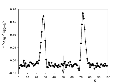
Figure 11: Correlator $y_{50}(t)\,y_{50+m}(t+20)$ as a function of the lattice coordinate $n$. $\beta$-FPU lattice, $N=101$, $T=2$. Arrow points to $n=50$

Two peaks in the correlation function, shifted by $m\approx\pm 25$, are visible. The velocity of their propagation is $v_{\rm p}=m/\tau\approx 1{.}25$.

III.1 Sound velocity in the $\beta$-FPU lattice

The temperature dependence of the sound velocity in the $\beta$-FPU lattice was discovered about a decade ago Lep98 . The sound velocity was estimated $v_{\rm snd}\sim\sqrt{1+\alpha}$, where $\alpha$ – parameter of renormalized frequencies depending on the temperature. Asymptotic value of the sound velocity in the high temperature limit $v_{\rm snd}\approx 1{.}22\,T^{1/4}$ was derived recently in Li_10 . If this formula apply to $T=2$ then $v_{\rm snd}\approx 1{.}45$ what differs from $v_{\rm p}\approx 1{.}25$ found from correlation functions above.

Below we derive more accurate expression for the sound velocity at low temperatures. It was shown Ala01 that in nonlinear systems there exists a spectrum of frequencies which are proportional to the harmonic ones, according to a well defined law. Then the $\beta$-FPU potential can be rewritten as

$$u(y)=\left(1+\dfrac{1}{2}y^{2}\right)\dfrac{1}{2}y^{2}$$ (19)

and an expression in brackets can be replaced by an effective rigidity $k_{\rm eff}$

$$u(y)=k_{\rm eff}\dfrac{1}{2}y^{2}.$$ (20)

As a result the lattice becomes harmonic and it is necessary to find $k_{\rm eff}$. It can be done in terms of mean field approximation (MFA). Mean value of potential energy is

$$\left<u_{\rm p}(y)\right>=k_{\rm eff}\dfrac{1}{2}\left<y^{2}\right>,$$ (21)

where $\left<y^{2}\right>$ is the mean of $y^{2}$. According to the virial theorem, mean values of potential and kinetic energies are equal in the harmonic lattice, that is $\left<u_{\rm p}\right>=\left<u_{\rm k}\right>$. But the identity $\left<u_{\rm k}\right>\equiv T/2$ holds for 1D systems. Then

$$k_{\rm eff}\dfrac{1}{2}\left<y^{2}\right>=\dfrac{T}{2}.$$ (22)

The condition of self consistency of the MFA is

$$\left(1+\dfrac{1}{2}\left<y^{2}\right>\right)=k_{\rm eff}$$ (23)

and it follows that $\left<y^{2}\right>=T/k_{\rm eff}$ and substitution of this expression into (23) gives the self-consistent equation for $k_{\rm eff}$:

$$1+T/(2k_{\rm eff})=k_{\rm eff}$$ (24)

with the solution

$$k_{\rm eff}=\dfrac{1}{2}+\sqrt{\dfrac{1}{4}+\dfrac{T}{2}}.$$ (25)

Eq. (25) defines the rigidity coefficient for the harmonic lattice with the renormalized spectrum depending on temperature $T$. Thereby the temperature renormalized sound velocity

$$v_{\rm snd}=\sqrt{k_{\rm eff}}=\sqrt{\frac{1}{2}+\sqrt{\frac{1}{4}+\frac{T}{2}}},\ \ (m=1)$$ (26)

and $v_{\rm snd}=1{.}27$ for $T=2$ what coincides with good accuracy with $v_{\rm p}\approx 1{.}25$ found from correlation functions. The high temperature asymptotic of the sound velocity $v_{\rm snd}\sim 0{.}84\,\left.T^{1/4}\right|_{T\gg 1}$. The temperature dependence of sound velocity for temperatures in the range $0\leq T\leq 10$ is shown in Fig. 13 and very good agreement between analytical and “experimental” results is observed.

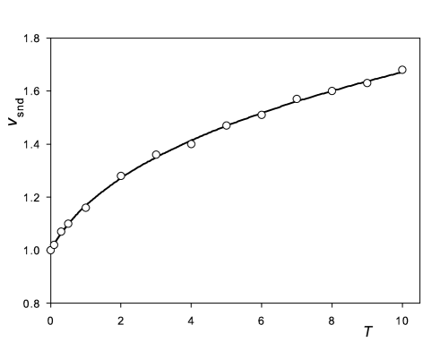
Figure 12: The temperature dependence of sound velocity $v_{\rm snd}$: solid line – dependence (26); empty circles – MD simulation.

If the mean field approximation is applied to the lattices with cubic nonlinearity $u(y)=\frac{1}{2}y^{2}\pm\frac{1}{3}y^{3}$ then no dependence of the sound velocity on temperature is expected. Really, $u(y)=\frac{1}{2}\left(1\pm\frac{2}{3}y\right)y^{2}$ and $k_{\rm eff}=\left(1\pm\frac{2}{3}\left<y\right>\right)=1$ as $\left<y\right>=1$.

The obtained results point to the fact that the nonlinearity can be also ignored in describing the thermodynamics of the $\beta$-FPU lattice, at least at $T<10$, and the harmonic lattice with renormalized rigidity coefficients (25) is an adequate model. This conjecture was checked at different temperatures $T=1,2,5,10$ by the comparison of the total energies computed in MD simulation of the $\beta$-FPU lattice and its harmonic model with renormalized rigidity coefficients. Very good coincidence of both energies testifies this hypothesis.

There exists an accurate expression for the specific potential energy (mean potential energy of one oscillator) Lik09

$$\dfrac{\left<U_{\rm p}\right>}{N}=\dfrac{1}{8}\left[\dfrac{K_{5/4}(q)+K_{3/4}(q)}{2\,K_{1/2}(q)}-1\right];\qquad q=1/(8T)$$ (27)

derived from the thermodynamics of the $\beta$-FPU lattice; $K$ – modified Bessel functions. Specific potential energy (27) and $\left<U_{\rm p}\right>/N$ computed in harmonic approximation with rigidity coefficients (25) coincidence with good accuracy.

III.2 Solitons and breathers in the $\beta$-FPU lattice

The discrete $\beta$-FPU lattice can be reduced to the modified Korteweg – de Vries (mKdV) equation in the continuum long-wavelength approximation (see Appendix). The mKdV equation has solutions in the form of solitons and moving breathers Lam80 .

Solitons of compression and elongation has the form

$$y(z,t)=\pm\dfrac{1}{\sqrt{6}}\,B\,{\rm sech}\left\{B\left[z-\left(1+\dfrac{B^{2}}{24}\right)t\right]\right\}$$ (28)

where plus/minus signs stand for elongation/compression solitons; $B$ – single parameter which simultaneously determines amplitude, width and velocity of soliton; $y$ – local deformation of the lattice; $z$ – soliton coordinate at time $t$.

The two-parameteric breather solution is

$$y(z,T)=-4\beta\,\mathrm{sech}{\Psi}\,\displaystyle\frac{\cos{\Phi}-(\beta/\alpha)\sin{\Phi}\,\mathrm{tanh}{\Psi}}{1+(\beta/\alpha)^{2}\sin^{2}{\Phi}\,\mathrm{sech}{\Psi}},$$ (29)

where

$$\begin{array}[]{ll}\Psi\equiv 2\beta(z-\gamma t)+\psi,&\Phi\equiv 2\alpha(z-\delta t)+\phi,\qquad{\rm and}\\ \gamma=4\,(3\alpha^{2}-\beta^{2}),&\delta=4\,(\alpha^{2}-3\beta^{2})\end{array}$$ (30)

and $\alpha,\beta$ are free parameters (see Appendix for more details). It is necessary to make transformation from continuous variables to discrete variables $y\to x_{i}-x_{i-1}$ and $z\to i$ in an attempt to use soliton and breather solutions on the discrete $\beta$-FPU lattice.

If soliton (28) and breather (29) solutions exist in the continuum limit, then the question arises: whether these moving localized excitations can be observed on discrete lattice? The answer is ‘yes’ and below the visualization method is suggested.

Recall that the visualization method for standing discrete breathers is well known Bik99 ; Aub06 : boundaries with friction forces absorb thermal noise (phonons) and standing breathers can be easily seen. Other method is necessary to visualize the moving excitations. Let we have the thermolized lattice with $N$ oscillators at temperature $T$. If “cold” lattice (with zero velocities and displacements) is switched to the thermalized lattice then solitons and breathers should “run out” to the cold lattice and could be observed. Results are shown in Fig. 13 and solitons and breather are immediately seen.

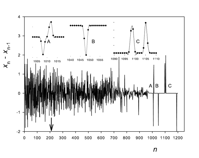
Figure 13: Solitons and breather running out of the initially thermalized lattice. A – breather, B – soliton of compression, C – pair of antisolitons (solitons of elongation). Arrow at $n=200$ shows the border separating initially thermalized and “cold” parts of the lattice. Initial temperature of the left lattice part ($1\leq n\leq 200$), $T=10$.

Solitons and breather (shown in inserts to Fig. 13) move faster then the sound front. At the first glance it is inconsistent with the relation between velocities of sound and solitons. The sound velocity at $T=10$ is $v_{\rm snd}\approx 1{.}67$ what is larger then the maximal soliton velocity $(v_{\rm sol})_{\rm max}\approx 1{.}3$ (see Appendix). But the temperature of expanding thermal excitations gradually decreases and the sound velocity also decreases according to (26). And there comes a point when solitons, which have constant velocity, keep ahead the sound front.

There are good grounds for believing that solitons and breathers do exist in the $\beta$-FPU lattice. Very likely that the soliton contribution to the heat conductivity increases with the growth of temperature. Really, the temperature dependence of the soliton density obeys the relation $n(T)\sim T^{1/3}$ for the Toda lattice at low temperatures Mar91 . Conceivably the growth of the solitons density with temperature might be an inherent property of nonlinear systems.

Our results on the soliton contribution to the heat conductivity are inconsistent with previous publication Li_10 where the energy carriers are effective phonons rather than solitons.

The possibility of energy transfer by solitons was conjectured three decades ago Tod79 . Less studied is the possibility of energy transfer by breathers. One suggested mechanism is the Targeted Energy Transfer Kop01 ; Man04 when an efficient energy transfer can occur under a precise condition of nonlinear resonance between discrete breathers. Various aspects and possible applications of energy transfer by breathers are considered in Aub06 .

IV Conclusions

In conclusion we briefly summarize our results. A new method for the calculation of the heat conductivity is suggested. This is done by the decomposing of the total dynamics into two parts: equilibrium process ${\bf x}^{0}(t)$ at equal temperatures $T$ of both lattice ends, and nonequilibrium process ${\bf x}^{1}(t)$ at temperature $\Delta T$ of one end and zero temperature of the other. This approach allows to extract and analyze the heat conductivity in an explicit form.

The primary goal of the paper was to develop a method which would allow to decrease the computational time at small temperature gradients when fluctuations of the heat flux are usually too large. It was supposed that at small temperature gradients, when the harmonic approximation is valid and an expression for the heat flux has the form (10), an analytical averaging over random Langevin noise terms can be done. This approach is very efficient for the calculation of quadratic in ${\bf x}^{1}(t)$ terms – the gain was thousand-fold. But formulaes are very complex for the linear terms and an efficient algorithm for their realization was not found yet. By this expedient the objective has not been met in full: the gain in computational time is obvious for small $(N\lesssim 100)$ lattices, but decreases as the lattice length increases. Nevertheless we suppose that the further analysis of process ${\bf x}^{1}(t)$ can be useful as it is responsible for the energy transfer.

The threshold phenomena are familiar in microcanonical ensembles Lic08 . There exists two values of specific energy $E$. One separates dynamical regime and weak chaos, and higher $E$ separates weak and strong chaos. It may be inferred that an existence of threshold phenomena is also a common occurrence in canonical ensembles. Really, a threshold temperature $T_{\rm thr}$ was found. The threshold temperature separates the different behavior of process ${\bf x}^{1}(t)$: process ${\bf x}^{1}(t)$ damps out at $T<T_{\rm thr}$ and reaches the stationary value at $T>T_{\rm thr}$. It may be conceived that the soliton and breather contributions to the heat conductivity increases with the growth of temperature if $T>T_{\rm thr}$. Solitons and breathers can emerge from either thermal fluctuations or higher order phonon interactions. Additional experiments for nanosized systems at low temperatures when $T<T_{\rm thr}$ can reveal some new features omitted in the present work.

The modified Korteweg – de Vries equation is derived in the continuum approximation for the $\beta$-FPU lattice. mKdV has solutions in the form of compression/elongation solitons and breathers. The stability of these quasi-particles was checked in numerical experiments. Both types of excitations were directly visualized.

On the other hand, it was found that the non-linear $\beta$-FPU lattice can be reduced to the harmonic lattice with the temperature renormalized frequency spectrum. This reduction allows to reproduce adequately the heat conductivity and thermodynamics of the parent lattice. These two, mutually contradictory, properties of the $\beta$-FPU lattice, – an inherent existence of solitons and breathers, and its “harmonic” behavior, seem to be very strange. Further analysis is necessary to solve this dilemma.

It is likely that some fraction of total heat conductivity is conditioned by solitons and moving breathers. But their contribution to the energy transfer deserves further investigation.

The $\beta$-FPU lattice is unique in the sense that in the continuum limit it has stable solutions in the form of solitons of compression and elongation. If the number of compression and elongation solitons is equal on average, then no macroscopic changes in the lattice length appear and an additional energy of deformation is negligible. It is an additional energetic factor favoring the solitons existence.

The case is quite different for unsymmetrical potentials which in the lowest order of the Taylor expansions have the form $u(y)=\frac{a}{2}y^{2}\pm\frac{b}{3}y^{3}$. $\alpha$-FPU, Toda, Morse, Lennard-Jones potentials are the examples. All these “cubic” potentials can be easily reduced to the ordinary KdV equation with the solution in the form of soliton of compression. And the large number of solitons is highly energetically unfavorable due to macroscopical compression of the lattice length.

Appendix A The modifief Korteweg – de Vries equation
for the $\beta$-FPU lattice. Solitons and breathers.

An approximate solution for the soliton of compression in the $\beta$-FPU lattice was obtained about two decades ago Wat93 . Analogous soliton solution with the profile $Q_{\rm snd}=\sqrt{2\,(v_{\rm snd}^{2}-1)}\,{\rm sech}\left[2\,z\sqrt{(v_{\rm snd}^{2}-1)/v_{\rm snd}^{2}}\,\right];\quad(z\sim x_{i}-x_{i-1})$ was used recently Li_10 and this solution is the function of a single parameter – sound velocity $v_{\rm snd}$.

Below we derive an equation for the continuum analogue of the $\beta$-FPU lattice with more accurate soliton and breather solutions. The $\beta$-FPU potential has general form

$$u(y_{i})=\dfrac{\alpha}{2}\,y_{i}^{2}+\dfrac{\beta}{4}\,y_{i}^{4};\quad(m=1),$$ (31)

where $y_{i}=x_{i}-x_{i-1}$ is the relative displacement of neighboring oscillators. The corresponding equations of motion are

$$\ddot{y}_{i}=\alpha\,\left(y_{i-1}-2y_{i}+y_{i+1}\right)+\beta\,\left(y_{i-1}^{3}-2y_{i}^{3}+y_{i+1}^{3}\right).$$ (32)

Starting from (32), the continuum approximation can be derived supposing small deviations from equilibrium. The series expansion in terms of $y_{i}$ up to the forth order is:

$$y_{i\pm 1}=y_{i}\pm y_{i}^{\prime}+\dfrac{1}{2}y_{i}^{\prime\prime}\pm\dfrac{1}{6}y_{i}^{\prime\prime\prime}+\dfrac{1}{24}y_{i}^{IV}\,.$$ (33)

Substitution of this expansion into (32) gives the continuum equation:

$$\ddot{y}=\alpha\left(y^{\prime\prime}+\dfrac{1}{12}y^{IV}\right)+3\beta\left(y^{2}\,y^{\prime}\right)^{2}\,.$$ (34)

Below we follow the well known reductive perturbation method (RPM) Sas81 ; Leb08 to get necessary equation in partial derivatives. The receipt consists in introducing new variables

$$\begin{split}y&=\varepsilon^{1/2}u_{1}+\varepsilon^{3/2}u_{2}+\ldots\,;\\ \xi&=\varepsilon^{1/2}(z-ct);\\ \tau&=\varepsilon^{3/2}t\,.\end{split}$$ (35)

Next the hierarchy of the expansions in terms of small parameter $\varepsilon$ should be used. If (35) is substituted in (34) and terms of the order $\varepsilon^{3/2}$ and higher are neglected, then $c^{2}(u_{1})_{\xi\xi}=\alpha(u_{1})_{\xi\xi}$ and $c=\sqrt{\alpha}$. $c$ is the sound velocity in the harmonic approximation. Transformation (35) means that the new coordinate system $\xi$ moves with velocity $c$ relative to the old coordinate system $z$.

Equation with the accuracy of the order $\varepsilon^{5/2}$ is

$$2c(u_{1})_{\tau}+3\beta(u_{1})^{2}(u_{1})_{\xi}+\dfrac{\alpha}{12}(u_{1})_{\xi\xi\xi}=0$$ (36)

and one can see that (36) reminds the well known modified KdV equation. Additional variables substitution $u_{1}=\sqrt{\alpha/6\beta}w$ and $\tau=(24/\sqrt{\alpha})T$ should be done to get the exact form of the mKdV equation:

$$w_{T}+6w^{2}w_{\xi}+w_{\xi\xi\xi}=0\,.$$ (37)

$\xi$ and $T$ are spatial and time variables.

Equation (37) has two types of solutions Lam80 . The soliton solution is

$$w(\xi,T)=\pm B\,{\rm sech}(B\xi-B^{3}T+\delta)=\pm B\,{\rm sech}[B(\xi-B^{2}T)-\xi_{0}]\,.$$ (38)

Plus/minus signs are related to elongation/contraction solitons, correspondingly. Soliton (38) is the one-parametric solution: free parameter $B$ defines simultaneously amplitude ($B$), half-width ($\sim 1/B$) and velocity ($B^{2}$); $\xi_{0}$ defines the soliton coordinate at $T=0$.

Returning back to initial coordinates $\left\{z,t\right\}$, the soliton solution is

$$y(z,t)=\pm\sqrt{\dfrac{\alpha}{6\beta}}\,B\,{\rm sech}\left\{B\left[z-\left(1+\sqrt{\alpha}{B^{2}}/{24}\right)t\right]-z_{0}\right\},$$ (39)

where $z$ – coordinate, $t$ – time, $z_{0}$ – soliton coordinate at $t=0$. The soliton velocity is $v_{\rm sol}=\sqrt{\alpha}(1+B^{2}/24)$ and is “supersonic” relative to the sound velocity in the harmonic approximation $v_{\rm snd}^{0}=\sqrt{\alpha}$. If $B$ increases then soliton has larger amplitude, becomes more narrow and its velocity increases. The soliton solution for the $\beta$-FPU lattice can be written if discrete variables in (39) are used: $y_{i}=x_{i}-x_{i-1}$, $z\to i$, $z_{0}\to i_{0}$.

Parameter $B$ can be arbitrary large in the continuum limit (39). But the lattice discreteness imposes limitations on the soliton width: solitons with the half-width less then $\lesssim 2.0$ become unstable. That is to say, soliton amplitude and velocity also have upper limit: $A=\sqrt{\alpha/6\beta}B\lesssim 1$,    $1\leq v_{\rm sol}\lesssim 1{.}3$ and the free parameter $B$ for discrete $\beta$-FPU lattice $B\lesssim\sqrt{6\beta/\alpha}$.

Two-parametric breather solution is

$$w(\xi,T)=-4\beta\,{\rm sech}\,\Psi\left[\dfrac{\cos\Phi-(\beta/\alpha)\sin\!\Psi\tanh\!\Psi}{1+(\beta/\alpha)^{2}\sin^{2}\!\Phi\,\,{\rm sech}\Psi}\right]\,,$$ (40)

where

$$\begin{split}\Psi\equiv 2\beta\xi-\gamma T-\psi,\quad&\Phi\equiv 2\alpha\xi-\delta T-\phi;\\ \gamma=8\beta(2\alpha^{2}-\beta^{2}),\quad&\delta=8\alpha(\alpha^{2}-3\beta^{2})\end{split}$$ (41)

$\alpha,\,\beta$ are free parameters; $\psi,\,\phi$ – initial phases; the group and phase velocities are $v_{\rm gr}=\gamma/2\beta$ and $v_{\rm ph}=\delta/2\alpha$, correspondingly. Returning back to coordinate system $z$, the breather solution takes the form

$$y(z,t)=-\sqrt{\dfrac{8\alpha}{3\beta}}\,\beta\,\,{\rm sech}{\widetilde{\Psi}}\,\dfrac{\cos{\widetilde{\Phi}}-(\beta/\alpha)\sin\!{\widetilde{\Phi}}\,\,{\rm tanh}{\widetilde{\Psi}}}{1+(\beta/\alpha)^{2}\sin^{2}\!{\widetilde{\Phi}}\,\,{\rm sech}{\widetilde{\Psi}}}\,,$$ (42)

where

$${\widetilde{\Psi}}\equiv 2\beta\left[z-\sqrt{\alpha}\left(1-\dfrac{\gamma}{48\beta}\right)t\right],\quad{\widetilde{\Phi}}\equiv 2\alpha\left[z-\sqrt{\alpha}\left(1-\dfrac{\delta}{48\alpha}\right)t\right]$$ (43)

and $\gamma,\delta$ are defined in (41).

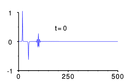
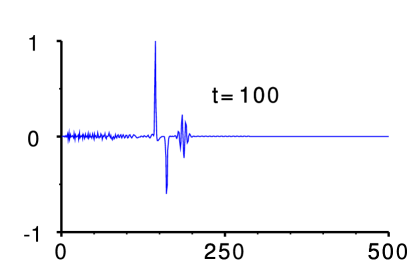
a                                                              b

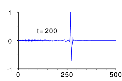
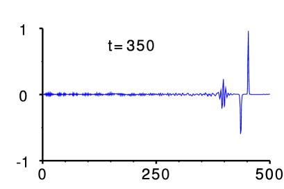
c                                                              d

Figure 14: Movement and collision of two solitons and one breather. Snapshots are made at $t=0,\,100,\,200,\,350$ t.u.

The group breather velocity $v_{\rm gr}=\sqrt{\alpha}(1-\gamma/48\beta)=\sqrt{\alpha}\,[1-(2\alpha^{2}-\beta^{2})/6]$. Its amplitude $\sim\sqrt{8\alpha\beta/3}$.

Soliton and breather stability was checked in numerical simulation. Initial conditions are chosen in the form of two solitons and one breather. Relative displacements are chosen according to (39) and (40), correspondingly. Velocities were obtained by differentiating by time.

The most left soliton of elongation has amplitude $A_{1}\simeq 1.09$ and velocity $v_{1}\simeq 1.3$ and initially located at $i_{1}=20$. Next soliton of compression has amplitude $A_{2}\simeq 0.63$ and velocity $v_{2}\simeq 1.1$ and initially located at $i_{2}=50$. Breather with parameters $\alpha=\pi/6,\,\,\beta=1/6$ is initially centered at $i_{3}=100$ and its velocity $v_{3}=0.91$ (see Fig. 14a). The velocities condition $v_{1}>v_{2}>v_{3}$ says that solitons and breather should meet and interact. This triple interaction is shown in Fig. 14c. But as result, all three species preserve their individuality (Fig. 14d). These findings (large free paths, preserving amplitudes and shapes after collision) unambiguously demonstrate that soliton and breather are do really exist in the $\beta$-FPU lattice

References

- (1) S. Lepri, R. Livi, A. Politi, Thermal conduction in classical low-dimensional lattices, Phys. Reports 377 (2003) 1–80.
- (2) E. Fermi, J. Pasta, S. Ulam, Document LA–1940 (May 1955); Collected papers of E. Fermi, University of Chicago Press, Chicago, 1965, vol. 2, p. 78.
- (3) CHAOS 15(1) (2005) (Focus Issue: The Fermi-Pasta-Ulam Problem – The First 50 Years, Ed. by D.K. Campbell, Ph. Rosenau, and G.M. Zaslavsky).
- (4) G. Gallavotti (Ed.), The Fermi-Pasta-Ulam Problem: A Status Report, Lect. Notes Phys. 728, Springer, Berlin Heidelberg, 2008.
- (5) M.D. Kruskal, N.J. Zabusky, Stroboscopis-perturbation procedure for treating a class of nonlinear wave equations, J. Math. Phys. 5 (1964) 231–244.
- (6) N.J. Zabusky, M.D. Kruskal, Interaction of “solitons” in a collisionless plasma and the recurrence of initial states, Phys. Rev. Lett. 15 (1965) 240–243.
- (7) R.K. Dodd, J.C. Eilbeck, J.D. Gibbon, H.C. Morris, Solitons and Nonlinear Wave Equations, Academic Press, New York, 1982.
- (8) D.K. Campbell, M. Peyrard, Heat conduction in a one-dimensional aperiodic system, Physica D 18 (1986) 47–53.
- (9) A. J. Sievers, S. Takeno, Intrinsic localized modes in anharmonic crystals, Phys. Rev. Lett. 61 (1988), 970–973.
- (10) T. Dauxois, M. Peyrard, Energy localization in nonlinear lattices, Phys. Rev. Lett. 70 (1993) 3935–3938.
- (11) S. Aubry, The concept of anti-integrability applied to dynamical systems and to structural and electronic models in condensed matter physics, Physica D 71 (1994) 196–221.
- (12) R.S. MacKay, S. Aubry, Proof of existence of breathers for time-reversible or hamiltonian networks of weakly coupled oscillators, Nonlinearity 7 (1994) 1623–1643.
- (13) M.A. Porter, N.J. Zabusky, B. Hu, D.K. Campbell, Fermi, Pasta, Ulam and the birth of experimental mathematics. A numerical experiment that Enrico Fermi, John Pasta, and Stanislaw Ulam reported 54 years ago continues to inspire discovery, American Scientist 97(3) (2009) 214–221.
- (14) P. Debye, Vorträge über die Kinetische Theorie der Wärme, Teubner, 1914.
- (15) G. Casati, B. Li, Heat conduction in one dimensional systems: Fourier law, chaos, and heat control, arXiv:cond-mat/0502546.
- (16) A.J. Lichtenberg, R. Livi, M. Pettini, S. Ruffo, Dynamics of oscillator chains, Lect. Notes Phys. 728 (2008) 21–121 .
- (17) . D. Barik, Anomalous heat conduction in a 2d Frenkel-Kontorova lattice, Europ. Phys. J. B 56 (2007) 229–234.
- (18) A. Lippi, R. Livi, Heat-conduction in two-dimensional nonlinear lattices, J. Stat. Phys. 100 (2000) 1147–1172.
- (19) K. Saito, A. Dhar, Heat conduction in a three dimensional anharmonic crystal, Phys. Rev. Lett. 104 (2010), 040601.
- (20) H. Shiba, N. Ito, Anomalous heat conduction in three-dimensional nonlinear lattices J. Phys. Soc. Jap. 77 (2008) 054006.
- (21) A. Henry, G. Chen, Anomalous heat conduction in polyethylene chains: Theory and molecular dynamics simulations, Phys. Rev. B 79 (2009) 144305/1–10.
- (22) Z. Yao, J.-S. Wang, B. Li, G.-R. Liu, Thermal conduction of carbon nanotubes using molecular dynamics, Phys. Rev B 71 (2005) 085417/1–8.
- (23) C. Yu, L. Shi, Z. Yao, D. Li, A. Majumdar, Thermal conductance and thermopower of an individual single-wall carbon nanotube, Nano Lett. 5 (2005) 1842–1846.
- (24) S. Maruyama, A molecular dynamics simulation of heat conduction in finite length SWNTs, Physica B 323 (2002) 193–195.
- (25) N. Mingo, and D.A. Broido, Length dependence of carbon nanotube thermal conductivity and the “problem of long waves”, Nano Lett. 5 (2005) 1221–1225.
- (26) J.X. Cao, X.H. Yan, Y. Xiao, J.W. Ding, Thermal conductivity of zigzag single-walled carbon nanotubes: Role of the umklapp process, Phys. Rev. B 69 (2004) 073407/1–4.
- (27) S. Lepri, R. Livi, A. Politi, Studies of thermal conductivity in Fermi-Pasta-Ulam-like lattices, CHAOS 15 (2005) 015118/1–9.
- (28) M. Toda, Solitons and heat conduction, Phys. Scr. 20 (1979) 424–430.
- (29) G. Friesecke, R.L. Pego, Solitary waves on the FPU lattices. I. Qualitative properties, renormalization and continuum limit, Nonlinearity 12 (1999), 1601–1628.
- (30) G. Friesecke, R.L. Pego, Solitary waves on the FPU lattices. II. Linear implies nonlinear stability, Nonlinearity 15 (2002), 1343–1360.
- (31) G. Friesecke, R.L. Pego, Solitary waves on the FPU lattices. III. Howland-type Floquet theory, Nonlinearity 17 (2004), 207–228.
- (32) G. Friesecke, R.L. Pego, Solitary waves on the FPU lattices. IV. Proof of stability at low energy, Nonlinearity 17 (2004), 229–252.
- (33) A. Hoffman, C.E. Wayne, Asymptotic two-soliton solutions in the Fermi-Pasta-Ulam Model, J. Dynamics and Diff. Equations 21 (2009) 343–351.
- (34) B. Li, J. Wang, L. Wang G. Zhang, Anomalous heat conduction and anomalous diffusion in nonlinear lattices, single walled nanotubes, and billiard gas channels, CHAOS 15 (2005) 015121/1–13.
- (35) H.J. Viljoen, L.L. Lauderback D. Sornette, Solitary waves and supersonic reaction front in metastable solids, Phys. Rev. E 65 (2002) 026609/1–13.
- (36) S. Maruyama, A molecular dynamics simulation of heat conduction of a finite length single-walled carbon nanotube, Microscale Thermophysical Engineering 7 (2003) 41–50.
- (37) K. Aoki, D. Kusnezov, Fermi-Pasta-Ulam -model: boundary jumps, Fourier’s law, and scaling, Phys. Rev. Lett. 86 (2001) 4029–4032.
- (38) K. Aoki, D. Kusnezov, Bulk properties of anharmonic chains in strong thermal gradients: non-equilibrium phi(4) theory, Phys. Lett. A 265 (2000) 250–256.
- (39) O.Narayan, S. Ramaswamy, Anomalous heat conduction in one-dimensional momentum-conserving systems, Phys. Rev. Lett. 89 (2002) 200601.
- (40) J.-S. Wang, Quantum thermal transport from classical molecular dynamics, Phys. Rev. Lett. 99 (2007) 160601/1-4.
- (41) Y. Zhang, H. Zhao, Heat conduction in a one-dimensional aperiodic system, Phys. Rev. E 66 (2002) 026106/1-4.
- (42) M. Johansson, G. Kopidakis, S. Lepri, S. Aubry, Transmission thresholds in time-periodically driven nonlinear disordered systems, Europh. Lett. 86 (2009) 10009.
- (43) Z. Rieder, J.L. Lebowitz, E.Lieb, Properties of a harmonic crystal in a stationary nonequilibrium state, J. Math. Phys. 8 (1967) 1073–1078.
- (44) S. Lepri, Relaxation of classical many-body Hamiltonians in one dimension, Phys. Rev. E 58 (1998) 7165–7171.
- (45) N. Li, B. Li, S. Flach, Energy carriers in the Fermi-Pasta-Ulam -lattice: solitons or phonons?, Phys. Rev. Lett. 105 (2010) 054102/1-4.
- (46) C. Alabiso, M. Casartelli, Normal modes on average for purely stochastic systems, J. Phys. A 34 (2001) 1223–1230.
- (47) V.N. Likhachev, T.Yu. Astakhova, W. Ebeling, G.A. Vinogradov, Equilibrium thermodynamics and thermodynamic processes in nonlinear systems, Eur. Phys. J. B 72 (2009) 247–256.
- (48) G. Lamb, Elements of soliton theory, John Willey & Sons, New York, 1980.
- (49) A. Bikaki, N.K. Voulgarakis, S. Aubry, G.P. Tsironis, Energy relaxation in discrete nonlinear lattices, Phys. Rev. E 59 (1999) 1234–1237.
- (50) S. Aubry, Discrete Breathers: Localization and transfer of energy in discrete Hamiltonian nonlinear systems, Physica D 216 (2006) 1–30.
- (51) F. Marchesoni, C. Lucheroni, Heat conduction in a one-dimensional aperiodic system, Phys. Rev. B 44 (1991) 5303–5305.
- (52) G. Kopidakis, S. Aubry, G.P. Tsironis, Targeted energy transfer through discrete breathers in nonlinear systems, Phys. Rev. Lett 87 (2001) 165501/1-4.
- (53) P. Maniadis, G. Kopidakis, S. Aubry, The concept of anti-integrability applied to dynamical systems and to structural and electronic models in condensed matter physics, Physica D 188 (2004) 153–177.
- (54) J.A. Wattis, Approximations to solitary waves on lattices. 2. Quasi-continuum methods for fast and slow waves, J. Phys. A 26 (1993) 1193–1209.
- (55) K. Sasaki, Solitons in one-dimensional helimagnets, Progr. Theor. Phys. 65 (1981) 1787–1797.
- (56) H. Leblond, The reductive perturbation method and some of its applications, J. Phys. B 41 (2008) 043001.