Soliton complexity in the damped-driven nonlinear Schrödinger equation: stationary, periodic, quasiperiodic complexes

Abstract

Stationary and oscillatory bound states, or complexes, of the damped-driven solitons are numerically path-followed in the parameter space. We compile a chart of the two-soliton attractors, complementing the one-soliton attractor chart.

I Introduction

This paper continues the study of localised time-periodic solutions of the parametrically driven damped nonlinear Schrödinger equation,

$$i\psi_{t}+\psi_{xx}+2|\psi|^{2}\psi-\psi=h\psi^{*}-i\gamma\psi.$$ (1)

(Here $h,\gamma>0$). Equation (1) is an archetypal equation for small and slowly-varying amplitudes of waves and patterns in spatially-distributed parametrically driven systems. It was employed to model intrinsic localised modes in coupled microelectromechanical and nanoelectromechanical resonators MEMS , solitons in dual-core nonlinear optical fibers DCF and dissipative structures in optical parametric oscillators OPO . The discrete version of (1) was studied as a prototype for the energy localisation in nonlinear lattices DB . (More contexts are listed in BZvH .)

In the previous publication BZvH , its authors proposed to obtain the time-periodic solitons as solutions of the two-dimensional boundary-value problem with the boundary conditions

$$\psi(x,t)\to 0\quad\text{as}\ x\to\pm\infty;\quad\psi(x,t+T)=\psi(x,t).$$ (2)

In the present paper, we apply this approach to the analysis of complexes of solitons.

Complexes (also known as molecules) are stationary or oscillatory associations of two or more solitons; they can be stable or unstable. Stable solitonic complexes, or bound states, were detected in a variety of soliton-bearing partial differential equations comp ; Mal_Par ; tails ; embed ; BZ1 ; water ; BW ; long_co ; Baer ; BZ2 . One mechanism of complex formation is the trapping of the soliton in a potential well formed by the undulating tail of its partner Mal_Par ; tails . This mechanism is not accessible Mal_Par to the parametrically driven damped solitons though, as their tails are decaying monotonically. The exchange of resonant radiation can also serve as a binding formula in nondissipative systems Mal_Par ; embed , but in the damped-driven equation (1) the radiation is nonresonant. A different mechanism was shown to operate here, which relies on the phase-stimulated growth or decay of the soliton’s mass BZ1 .

Bound states serve as long-term attractors in situations where there is more than one soliton present in the initial condition. For example, two like-polarity surface solitons in a vertically-driven water tank attract each other and form a stable bound state water . Unstable complexes do not have the same experimental visibility and can appear only as transients in numerical simulations. However, unstable complexes have a mathematical role to play: they work as the phase-space organisers BW .

The formation of complexes with an increasing number of elementary constituents long_co gives rise to a higher degree of spatial complexity in the system, in the same way as the binding of shorter molecules into longer ones produces chemical compounds with increasingly complex properties. Previous analyses were confined to stationary BZ1 and steadily moving Baer ; BZ2 associations of the parametrically driven solitons. In the present paper we extend these studies to time-periodic complexes, thereby increasing the temporal complexity of the localised structures.

We consider time-periodic complexes as “stationary” solutions of Eq.(1) on a two-dimensional domain $-\infty<x<\infty$, $0\leq t\leq T$. This allows to determine both stable and unstable complexes. Solutions of the boundary-value problem (1), (2) are path-followed in the parameter space — in the same way as free-standing periodic solitons were continued in the previous publication BZvH .

An outline of this paper is as follows. In the next section we describe bifurcations of the static two-soliton complexes. Of particular importance here are the Hopf bifurcations; these give birth to time-periodic solutions. We establish that the values of the damping coefficient are divided into two ranges. Namely, for $\gamma$ larger than a certain threshold, the complex suffers one or more Hopf bifurcations as $h$ is varied. Below the threshold $\gamma$, no Hopf bifurcations occur.

In section III, the Hopf-bifurcation points of the stationary complexes are exploited as the starting points of the $T(h)$ curves for the time-periodic complexes. These curves are traced as we continue the periodic bound states in a parameter. Depending on the number of the Hopf bifurcations suffered by the static complex, we have one, two or more branches of the periodic solutions emanating out of it. Complexes resulting from different Hopf bifurcations follow different transformation routes.

In the concluding section (section IV) the results on stationary and time-periodic complexes are summarised in the form of a two-soliton attractor chart. Included in this chart are also some quasiperiodic attractors.

II Stationary two-soliton complexes

The two free-standing stationary soliton solutions to Eq.(1) are distinguished by the subscripts $+$ and $-$:

$$\psi_{\pm}(x)=A_{\pm}\exp(-i\theta_{\pm})\,{\rm sech\/}(A_{\pm}x),$$ (3)

where

$$A_{\pm}=\sqrt{1\pm\sqrt{h^{2}-\gamma^{2}}},\quad\theta_{+}=\frac{1}{2}\arcsin\frac{\gamma}{h},$$

and $\theta_{-}=\pi/2-\theta_{+}$. The $\psi_{-}$ soliton is unstable for all $h$ and $\gamma$. The soliton $\psi_{+}$ is stable when the difference $h-\gamma$ is small but loses its stability to a time-periodic soliton when $h$ exceeds a certain limit $h_{\rm Hopf}(\gamma)$.

The solitons $\psi_{+}$ and $\psi_{-}$ can form a variety of bound states, or complexes BZ1 ; BZ2 ; Baer . (For example, in the previous paper BZvH we mentioned a complex $\psi_{(-+-)}$, that is, a symmetric stationary association of two solitons $\psi_{-}$ and one $\psi_{+}$.) All complexes involving the $\psi_{-}$ solutions are, expectably, unstable; however two $\psi_{+}$ solitons can form a stable bound state BZ1 .

Previously, the two-soliton complex $\psi_{(++)}$ was known to exist only for sufficiently large values of damping BZ1 ; BZ2 . We have now established that this complex exists for all $\gamma\geq 1.5\times 10^{-8}$. Its domain of existence on the $(\gamma,h)$-plane is not bounded from above except that for $h$ greater than

$$h_{\rm cont}=\sqrt{1+\gamma^{2}},$$

the complex is unstable to the continuous-spectrum perturbations (as any other solution decaying to zero at the infinities). Reducing $h$ from $h_{\rm cont}$ for the fixed $\gamma$, we obtain one of two possible types of bifurcation diagrams on the $(h,E)$ plane, where the energy $E$ is defined by

$${E}=\int_{-\infty}^{\infty}\left[|\psi_{x}|^{2}+|\psi|^{2}-|\psi|^{4}+h\frac{\psi^{2}+{\psi^{*}}^{2}}{2}\right]dx.$$ (4)

(The energy is not an integral of motion when $\gamma\neq 0$; however, $E$ is obviously a constant for time-independent solutions and can be used as a physically meaningful bifurcation measure.)

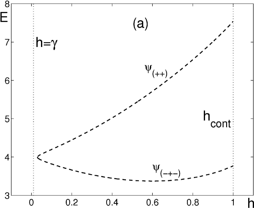
Figure 1: Energy of the stationary two-soliton complex and stationary multisoliton solutions obtained from this complex by continuation in $h$ for the fixed $\gamma$. (a) $\gamma=0.01$; (b) $\gamma=0.4$. Solid curves show stable and the dashed ones unstable solutions. Note two intervals of stability of the $\psi_{(++)}$ complex in (b).

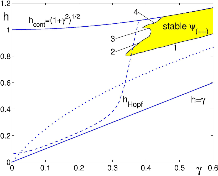
Figure 2: (Color online) The existence and stability domains of the stationary two-soliton complex $\psi_{(++)}$. The region of existence of the complex is bounded from below by the dotted line; in the upwards direction it extends beyond the value $h_{\rm cont}$, without bound. The complex is stable only in a small part of this region [tinted yellow (light gray)]. The stability domain is bounded by the curve $h=h_{\rm cont}(\gamma)$ on the top and by the lines of four Hopf bifurcations (1, 2, 3, and 4) on other sides. The dashed curve is the line of the Hopf bifurcation of the single soliton $\psi_{+}$. (The soliton is unstable above this line.)

The diagram of the first type [Fig.1(a)] arises when $h$ is decreased for a fixed small $\gamma$ ($\gamma\leq 0.292$). In this case, there is only one turning point, $h=h_{\rm sn}$, with $h_{\rm sn}=h_{\rm sn}(\gamma)>\gamma$. [For the parameter value $\gamma=0.01$ which we used to create Fig.1(a), $h_{\rm sn}=0.02972$; for $\gamma=0.1$, the turning point is at $h_{\rm sn}=0.25$, and for $\gamma=0.25$, $h_{\rm sn}=0.49$.] As $h$ approaches $h_{\rm sn}$ along the top branch, the two-soliton solution $\psi_{(++)}$ develops a third hump halfway between the two humps that are already there, with the distance between the lateral humps remaining unaffected by this development. The complex obtained by the continuation of this solution to the bottom branch can be identified as a three-soliton bound state $\psi_{(-+-)}$. As we continue away from $h_{\rm sn}$ along the bottom branch in Fig.1(a), the $\psi_{-}$ solitons bound in this complex (the two side solitons) diverge to the infinities on the $x$ axis.

All branches in the diagram of the first type consist of unstable solutions. (Our approach to the stability analysis of stationary solutions has been outlined in BZvH .)

A somewhat different diagram arises for larger values of $\gamma$ ($\gamma>0.292$), see Fig.1(b). This bifurcation diagram has been described in BZ1 for a particular $\gamma$ ($\gamma=0.565$); here, we reproduce it for a different value of the damping coefficient. Reducing $h$ from $h_{\rm cont}$ for the fixed $\gamma$, the branch resulting from the two-soliton solution $\psi_{(++)}$ develops two turning points instead of one. As we pass the first turning point, the $\psi_{(++)}$ complex transforms into the $\psi_{(--)}$ solution. Moving away from the point along the bottom branch, the $\psi_{(--)}$ complex acquires a third hump. This branch does not continue all the way to $h_{\rm cont}$ but turns again, into a branch with even a lower energy. On this branch, the three-hump solution can be identified as $\psi_{(-+-)}$. The lowest branch continues to the point $h=\gamma$. This point defines the lower boundary of the domain of existence of the stationary complexes which result from the path-following of the two-soliton solution $\psi_{(++)}$. As we approach the point $h=\gamma$, the distance between the two side solitons in the $\psi_{(-+-)}$ complex tends to infinity.

For $\gamma$ just above $0.292$, all solution branches in the diagram of the second type are unstable. However, as $\gamma$ exceeds $0.34$, a stability window opens in the $\psi_{(++)}$ branch. The existence and stability domains of the two-soliton complexes on the $(\gamma,h)$ plane are shown in Fig.2.

We were not able to obtain a symmetric two- or three-soliton complex for $\gamma=0$. If we fix $h$ and continue in $\gamma$ towards $\gamma=0$, the separation distance between the solitons in the complex grows without bounds; hence we conjecture that symmetric multisoliton complexes do not exist for $\gamma=0$. (There are nonsymmetric complexes with $\gamma=0$ though; see Baer .)

The shape of the $E(h)$ curve corresponding to $\gamma=0.4$ [Fig.1(b)] looks similar to that of the $E(h)$ curve for $\gamma=0.565$ BZ1 . The main difference between the diagrams pertaining to these two values of $\gamma$ is that when $\gamma=0.565$, the stability region of the two-soliton solution is seamless, i.e. does not have instability gaps in it, whereas in the $\gamma=0.4$ case, the stability region consists of two segments of the curve separated by an interval of instability. This difference is reflected by the shape of the stability domain on the $(\gamma,h)$-plane (note the “instability bay” on the north-west coast of the stable region in Fig.2).

Each point of the “coastline” of the stability “continent” in Fig.2 corresponds to a Hopf bifurcation of the stationary complex [except for points along the curve $h=h_{\textrm{cont}}(\gamma)$]. The “coastline” consists of four segments (marked 1, 2, 3, and 4 in Fig.2). Continuing in $h$ along a vertical line $\gamma=const$ one crosses one, two or four of these; accordingly, for a given $\gamma$, the complex may undergo one, two or four Hopf bifurcations.

III Time-periodic complexes

The first segment (marked 1 in Fig.2) is defined as the “south coast” of the tinted continent. It extends from $\gamma=0.34$ to larger $\gamma$ without a visible bound — presumably all the way to $\gamma=\infty$. The line of the second Hopf bifurcation (marked 2) represents the “north coast of the southern peninsula” in Fig.2; it is bounded by $\gamma=0.34$ on the left and $\gamma=0.413$ on the right. The “south coast of the northern peninsula” corresponds to the third Hopf bifurcation (marked 3); this extends from $\gamma=0.39$ to $\gamma=0.413$. Finally, the top, fourth, Hopf bifurcation arises for $\gamma$ between $0.39$ and $0.445$ (marked 4). When $\gamma$ is greater than $0.445$, the complex undergoes just one Hopf bifurcation as $h$ varies (the one marked 1).

III.1 The first Hopf bifurcation

In this subsection, we path-follow time-periodic complexes born in the lowest Hopf bifurcation (i.e. detaching from the south coast of the tinted “continent” in Fig.2). We take $\gamma=0.565$ as a representative value of damping in the region where the stationary two-soliton complex undergoes only one Hopf bifurcation and $\gamma=0.35$ and $0.38$ in the region where there is more than one Hopf point.

When $\gamma=0.565$, the (only) Hopf bifurcation is at $h_{H1}=0.94$. Using this value as a starting point in our continuation process, results in the bifurcation diagram shown in Fig.3(a). In order to articulate details of the diagram, we supplement the graph of the period $T(h)$ with a plot of the averaged energy, defined by

$${\overline{E}}=\frac{1}{T}\int_{0}^{T}E(t)\,dt,$$ (5)

where $E(t)$ is given by Eq.(4). We also evaluate Floquet multipliers as described in BZvH .

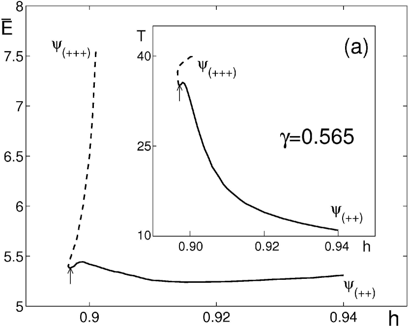
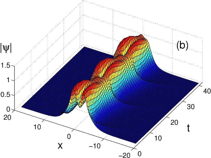
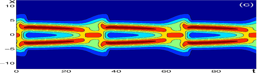
Figure 3: (Color online) (a) The average energy (main panel) and the period (inset) of the periodic solution arising for $\gamma=0.565$. The solid curve shows the stable and the dashed one unstable branch. The point of the period-doubling bifurcation is marked by a vertical arrow. (b-c) Representative solutions on the lower branch in panel (a). (b): $h=0.92$, $T=13.973$; shown is the absolute value of $\psi$. (c): $h=0.90$, $T=32.729$; shown are the level curves of $|\psi|$. The time interval covered by (b) and (c) includes three periods of oscillation.

At the starting point $h_{H1}=0.94$, the Floquet spectrum includes three unit eigenvalues and two complex-conjugate pairs with moduli smaller than one. As $h$ is decreased from $h=0.94$, two unit eigenvalues remain in the spectrum while the third one moves inside the unit circle along the real axis. This positive eigenvalue decreases in modulus until it passes to the negative semiaxis at $h=0.92$; once the eigenvalue has become negative, it starts growing in absolute value. Eventually, as $h$ reaches the value of $0.897$, the negative real eigenvalue crosses through $\mu=-1$. A period-doubling bifurcation occurs at this point; as $h$ drops below $0.897$, the periodic complex becomes unstable but a stable double-periodic solution is born. Note that the destabilization occurs not at the turning point of the ${\overline{E}}(h)$ curve (which is at $h=0.89665$) but for a slightly larger $h$, i.e. before the turning point is reached. Fig.3(b) shows a representative solution on the lower, “horizontal”, branch of the ${\overline{E}}(h)$ curve.

As for the two complex pairs, the eigenvalues constituting one of these grow in absolute value as we move along the “horisontal” branch towards smaller $h$. At the same time, the imaginary parts of these eigenvalues decrease and the pair converges on the positive real axis — just before crossing through the unit circle. The two real eigenvalues cross through $\mu=1$ almost simultaneously, as the curve turns back at $h=0.89665$; after that, they remain outside the unit circle. The other complex pair also converges on the real axis but remains inside the unit circle along the entire curve.

As $h$ is decreased and we approach the turning point in Fig.3(a), the amplitude of oscillations grows and the solution transforms into a sequence of soliton fusions and fissions. Two solitons merge into one entity which then breaks into two constituents, and this process continues periodically; see Fig.3(c).

The whole of the “vertical” branch of the ${\overline{E}}(h)$ curve is unstable. The branch ends at the stationary $\psi_{(+++)}$ solution (here $h=0.901$). As we approach the endpoint of this branch, the two real (positive) eigenvalues with $\mu<1$ and one of the two eigenvalues with $\mu>1$ move closer to 1. At the endpoint, the spectrum includes three unit eigenvalues and two real eigenvalues close to $1$. This corresponds to the spectrum of a stationary three-soliton complex near its Hopf boifurcation.

Proceeding to the region with more than one Hopf point, we consider $\gamma=0.35$. Here, the “lower” Hopf bifurcation occurs at $h_{H1}=0.805$. This bifurcation is supercritical; as $h$ drops below $h_{H1}$, the stationary two-soliton bound state loses its stability to a periodic two-soliton complex which is born at this point. At the bifurcation point, the spectrum of the Floquet multipliers includes three unit eigenvalues and two complex-conjugate pairs inside the unit circle — one with ${\rm Re\/}\,\mu<0$ and the other one with ${\rm Re\/}\,\mu>0$. As we continue the periodic complex towards smaller $h$, the negative-real-part pair converges on the real axis inside the unit circle, after which one of the resulting negative eigenvalues grows in absolute value and, at $h=0.79$, crosses through $\mu=-1$. The periodic complex loses its stability to a double-periodic bound state of two solitons. As we continue the unstable branch, it makes a number of turns (Fig.4(a)), the spatiotemporal complexity of the solution increases (Fig.4(b)) but it never regains its stability.

Another representative value of $\gamma$ with two Hopf bifurcations, is $0.38$. Here, the continuation of the two-soliton complex from the lower Hopf point results in the $T(h)$ curve similar to the $\gamma=0.35$ case (Fig.4(a)). Like in the $\gamma=0.35$ case, the solution loses stability in a period-doubling bifurcation. We did not path-follow the unstable branch far beyond the bifurcation point.

Summarising results of continuation from the first, “lowest”, Hopf bifurcation in Fig.2, we note that the bifurcation is supercritical — both for large and small $\gamma$. Another common feature is the loss of stability resulting from a Floquet multiplier crossing through $\mu=-1$. Since this bifurcation occurs before the first turn of the $T(h)$ curve, it always gives rise to a stable double-periodic solution. It is also fitting to note that all time-periodic complexes emerging in the first Hopf bifurcation are symmetric in space (i.e. invariant under the reflection $x\to-x$).

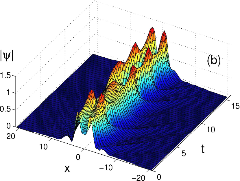
Figure 4: (Color online) The first branch of the two-soliton time-periodic complex for $\gamma=0.35$ and $\gamma=0.38$. (a): the period of the solution. The solid curves show the stable and the dashed ones unstable branches. The circles mark the starting points of the continuation (the stationary complex $\psi_{(++)}$). (b): A two-soliton periodic solution with complex temporal behaviour arising at the end point of the $\gamma=0.35$ curve in (a). (Here $h=0.741$, $T=15.9$.) The figure shows just one period of oscillation.

III.2 The second and the third Hopf bifurcations

When $\gamma$ lies between $0.34$ and $0.39$, the stationary two-soliton complex suffers two Hopf bifurcations, at $h_{\textrm{H1}}$ and $h_{\textrm{H2}}$, with $h_{\textrm{H2}}>h_{\textrm{H1}}$. (These are marked 1 and 2 in Fig.2.) In this subsection, we describe the continuation of periodic solutions detaching at $h_{\textrm{H2}}$ (the second of the two bifurcations) for several representative values of damping.

The second Hopf bifurcation is subcritical: the emerging periodic branch is unstable and coexists with the stable stationary branch. That is, the periodic branch initially extends down in $h$, see the $\gamma=0.35$ and $\gamma=0.38$ curves in Fig.5. At some point the branch turns back after which $h$ grows without any further U-turns; notably, it grows beyond the interval of the stable stationary bound states (Fig.5).

The periodic branch ends at an unstable stationary complex. The endpoint corresponds to the “concealed” Hopf bifurcation of the stationary solution where a pair of complex-conjugate eigenvalues crosses from one half of the complex plane to the other but the solution remains unstable due to additional unstable eigenvalues.

When $\gamma$ is set on $0.35$, the whole periodic branch is unstable but for $\gamma$ as close as $0.36$ a narrow stability window appears inside it. As $\gamma$ grows from $0.36$, the stability window expands — see the $\gamma=0.38$ curve in Fig.5 which features a sizeable stability interval $h_{1}<h<h_{2}$, with $h_{1}=0.9415$ and $h_{2}=1.015$. Within this stability window, the periodic complex has two complex-conjugate pairs of Floquet multipliers $\mu_{4}=\mu_{3}^{*}$ and $\mu_{6}=\mu_{5}^{*}$, with $|\mu|<1$ (in addition to two unit eigenvalues). As $h$ is decreased below $h_{1}$, the first pair ($\mu_{3,4}$) moves outside the unit circle, with the second pair remaining inside; when $h$ is raised above $h_{2}$, the unit circle is crossed by the second pair ($\mu_{5,6}$), with the first pair remaining inside. Thus the stability interval is bounded by the Neimark-Sacker bifurcation on each side. This observation suggests that a quasi-periodic two-soliton complex should be born on the crossing of either stability boundary, $h_{1}$ and $h_{2}$ — the conclusion confirmed by direct numerical simulations of Eq.(1). (Quasiperiodic solutions can obviously not be captured by the periodic boundary-value problem; the direct numerical simulation remains the only feasible way of determining them.)

It is worth mentioning here that the periodic two-soliton complexes coexist with periodic one-soliton solutions. (For example, for $\gamma=0.35$, the periodic free-standing soliton exists between $h=0.75$ and $h=1.02$; see Fig.2 in BZvH .) However the one- and two-soliton branches are not connected.

When $\gamma$ is between $0.39$ and $0.413$, the stationary complex undergoes four Hopf bifurcations, $h_{\textrm{H1}}<h_{\textrm{H2}}<h_{\textrm{H3}}<h_{\textrm{H4}}$ (marked 1, 2, 3, 4 in Fig.2.). This is the interval of $\gamma$ that contains the top “peninsula” in Fig.2. Choosing $\gamma=0.41$ as a representative value of damping, we path-followed the periodic complex which is bifurcating off at the point $h_{\textrm{H2}}$. Like in the case $0.34<\gamma<0.39$ discussed above, the bifurcation is subcritical: the emerging periodic branch is unstable and initially extends down in $h$. As in the previously discussed case, the $T(h)$ curve turns (at $h=h_{\textrm{tn}}=0.9447$) and the entire subsequent continuation proceeds in the direction of increasing $h$ (Fig.5).

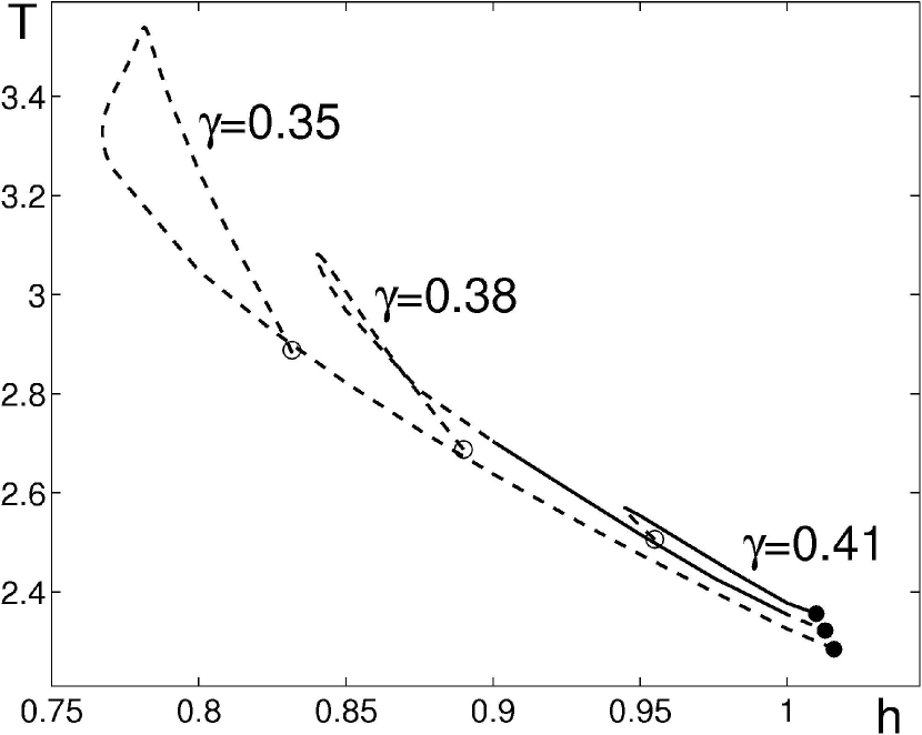
Figure 5: The second branch of the periodic two-soliton solution. The empty circles mark the starting points of the continuation — the points $h=h_{\textrm{H2}}$ where the stationary two-soliton complex suffers the second Hopf bifurcation. The full circles mark the endpoints. The endpoint of the $\gamma=0.41$ curve corresponds to the third Hopf bifurcation ($h_{\textrm{H3}}$); the endpoints of the $\gamma=0.35$ and $\gamma=0.38$ curves lie inside the instability domain of the stationary complex. The solid curves show the stable and the dashed ones unstable branches.

To describe the motion of the Floquet multipliers, it is convenient to start somewhere within the “upper” part of the $\gamma=0.41$ branch, e.g. at $h=0.99$. At this point, the spectrum of linearisation includes two pairs of complex-conjugate multipliers $\mu_{4}=\mu_{3}^{*}$, $\mu_{6}=\mu_{5}^{*}$, both with $|\mu|<1$. However, in contrast to the previously discussed scenario, neither of these two pairs crosses through the unit circle as $h$ is inceased or decreased and so the periodic complex with this $\gamma$ does not experience any Neimark-Sacker bifurcations.

As $h$ is decreased from $0.99$, the multipliers $\mu_{3,4}$ converge on the real axis and, at the turning point $h_{\textrm{tn}}$, cross through $\mu=1$ (almost simultaneously). The other complex pair, $\mu_{5,6}$, remains inside the unit circle. Therefore, the turning point corresponds to a saddle-node bifurcation of limit cycles. If we, instead, increase $h$ starting at $h=0.99$, it is the $\mu_{5,6}$ pair that converges on the real axis, just before $\mu_{5}$ becoming equal to one. At this point the periodic branch rejoins the branch of stationary complexes; this value of $h$ is nothing but $h_{\textrm{H3}}$, the point of the third Hopf bifurcation of the stationary two-soliton bound state. At $h=h_{\textrm{H3}}$, the Floquet spectrum includes three unit eigenvalues, a real eigenvalue $\mu_{6}$ close to (but smaller than) one, and a complex-conjugate pair $\mu_{3,4}$ inside the unit circle. Thus the periodic complex remains stable in the whole range between the turning point $h_{\textrm{tn}}$ and the point $h_{\textrm{H3}}$ where it rejoins the (stable) stationary branch.

Since the saddle-node bifurcation point $h_{\rm tn}$ lies below $h_{\rm H2}$, there is an interval $h_{\rm tn}\leq h\leq h_{\rm H2}$ where we have bistability between the stationary and time-periodic two-soliton complexes.

In summary, the second Hopf bifurcation is always subcritical; the continuation connects it either to the third (supercritical) Hopf bifurcation, or to a concealed bifurcation of unstable two-soliton complexes. All time-periodic solutions arising in these bifurcations are symmetric in space.

III.3 The fourth, symmetry-breaking, Hopf bifurcation

The locus of the fourth Hopf bifurcation is a stretch of the north-west coast of the “continent” of stable stationary complexes in Fig.2 (marked 4). The “north-western coastline” extends from $\gamma=0.39$ to the point $\gamma=0.445$, where it meets the continuous-spectrum instability curve $h=h_{\textrm{cont}}(\gamma)$. At the bifurcation point a pair of complex eigenvalues $\lambda,\lambda^{*}$ of the eigenvalue problem

$$(\mathcal{H}-\gamma J){\bf p}(x)=\lambda J{\bf p}(x),$$

cross through the imaginary axis. Here $\mathcal{H}-\gamma J$ is the operator of linearisation about the stationary solution (see BZvH for details). The bifurcation is symmetry breaking: unlike three other Hopf bifurcations, the corresponding eigenfunctions ${\bf p}(x)$ and ${\bf p}^{*}(x)$ are odd (antisymmetric): ${\bf p}(-x)=-{\bf p}(x)$. Accordingly, the time-periodic solutions which are born in this bifurcation describe out-of-phase oscillations of two identical solitons making up the complex [see Fig.6(b)].

The fourth Hopf bifurcation is supercritical: the emerging periodic branch is stable and extends up in $h$. For $\gamma=0.41$ which we take as a representative value of damping, this bifurcation occurs at $h_{\rm H4}=1.037$. At the bifurcation point, the Floquet spectrum includes three eigenvalues $\mu_{1,2,3}=1$, two real positive multipliers $\mu_{4,5}<1$ and several complex-conjugate pairs with $|\mu|<1$. As $h$ grows from $h_{\textrm{H4}}$, one of the unit eigenvalues moves inside the unit circle, but as $h$ is further increased, it reverses and moves out. At this point ($h=1.049$), a saddle-node bifurcation of cycles occurs; the periodic solution loses its stability and the branch turns back [Fig.6(a)]. As we continue it further, the real and complex eigenvalues move back and forth through the unit circle; some pairs converge on the real axis — but the solution never regains its stability.

After a lengthy excursion into the $(h,T)$ plane [Fig.6(a)], the periodic branch rejoins the branch of (unstable) stationary complexes $\psi_{(++)}$ (at $h_{\textrm{cnc}}=1.082$). The spectrum of the endpoint stationary solution includes three unit eigenvalues, a positive eigenvalue $\mu_{4}<1$, and two complex-conjugate pairs, with $|\mu_{5,6}|<1$ and $|\mu_{7,8}|>1$. The value $h=h_{\textrm{cnc}}$ pertains to the concealed Hopf bifurcation of the unstable stationary complex $\psi_{(++)}$.

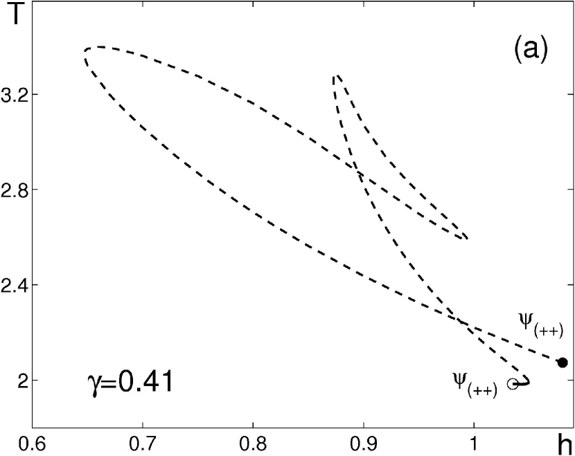
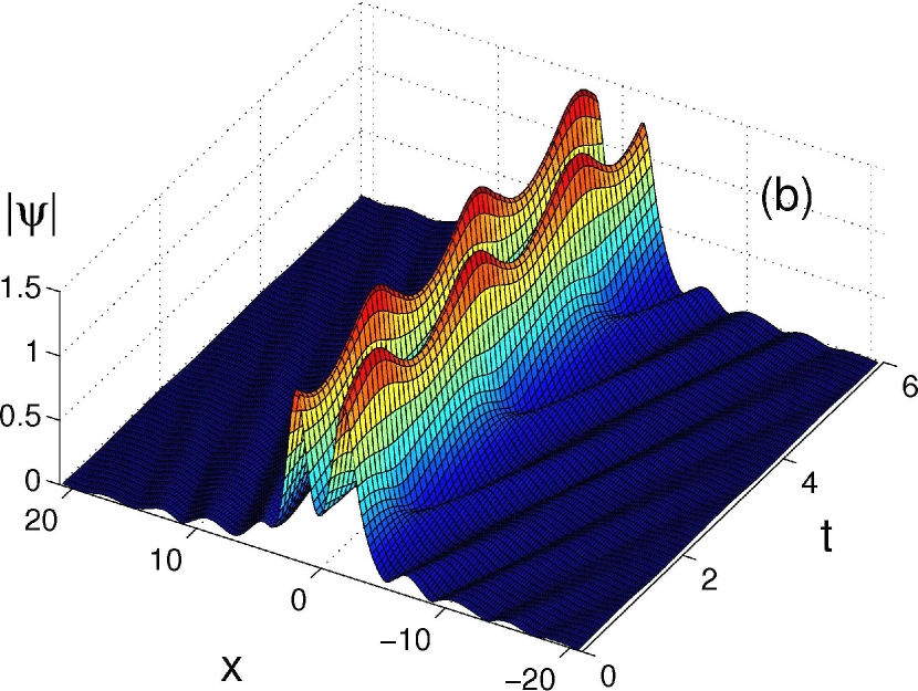
Figure 6: (Color online) (a) The branch of periodic 2-soliton complexes oscillating out of phase with each other. The empty circle marks the starting point of the continuation — the point $h=h_{\textrm{H4}}$ where the stationary two-soliton complex suffers the symmetry-breaking Hopf bifurcation. The full circle marks the endpoint. The short solid segment near the beginning of the curve represents the stable solution; the rest of the branch (dashed) is unstable. (b) A representative solution on the stable part of this branch. Here $h=1.0493$ and $T=1.991$; several periods of oscillation are shown.

IV The two-soliton attractor chart and open problems

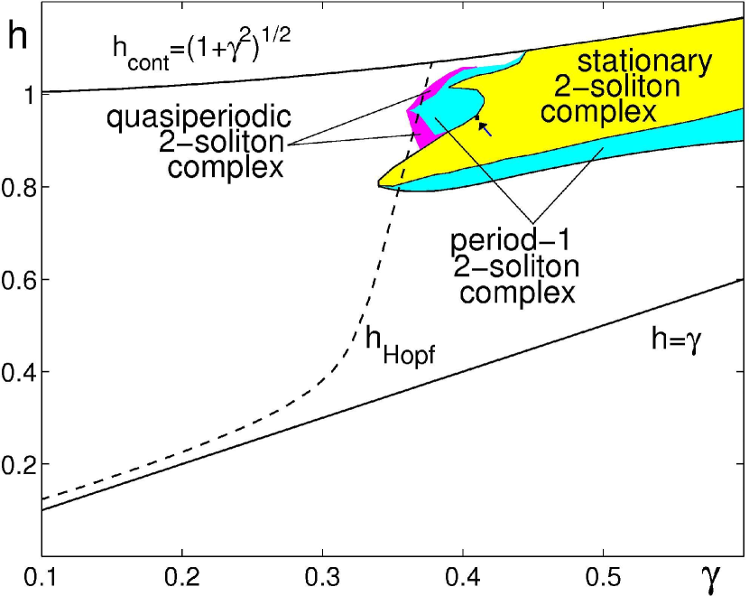
Figure 7: (Color online) Two-soliton attractor chart. The chart is still under construction; the outer boundaries of the purple (dark gray) area (populated by quasiperiodic two-soliton attractors) are still to be refined. The black mark (pointed to by the arrow) initiates the periodic/stationary bistability region. The dashed curve is the line of the Hopf bifurcation of the $\psi_{+}$ soliton, shown just for the reference purposes.

Fig.7 summarises our results on the stationary and periodic two-soliton attractors. This diagram complements the single-soliton attractor chart compiled in the first part of this project BZvH . The two-soliton chart is in qualitative agreement with results of direct numerical simulations Wang .

In Fig.7, we have included stable quasiperiodic complexes [highlighted in purple (dark gray)]. The boundaries between the stable-periodic and stable-quasiperiodic domains are defined by the Neimark-Sarker bifurcations of the periodic complexes; these admit an accurate demarcation using our method (i.e. by monitoring the Floquet multipliers along the periodic branches). On the other hand, in order to determine where the stable quasiperiodic solution ceases to exist, we had to relinquish our continuation approach in favour of direct numerical simulations of Eq.(1). We have performed only a few runs and hence Fig.7 gives only a schematic position of the outer boundary of the quasiperiodic stability domain. In order to demarcate this boundary more accurately, one would need to perform numerical simulations more extensively. This is beyond the scope of our present study.

The region of bistability of stationary and periodic complexes also needs to be accurately delimited. So far, we have only demarcated a small portion of it; see the black mark in Fig.7.

Finally, it would also be interesting to continue periodic solutions bifurcating from the stationary complexes in the “concealed” Hopf bifurcations, where the stationary solution remains unstable on both sides of the bifurcation due to additional eigenvalues with positive real parts. In our continuation process bifurcations of this sort would typically arise as the endpoints of the periodic branches starting at the proper Hopf bifurcations of the stationary complexes. Starting at the concealed bifurcations would produce an additional wealth of periodic branches some of which may have stable segments.

- (1) I V Barashenkov, E V Zemlyanaya, T C van Heerden, previous submission
- (2) E. Kenig. B. A. Malomed, M.C. Cross, and R. Lifshitz, Phys. Rev. E 80, 046202 (2009); M. Syafwan, H. Susanto, and S. M. Cox, Phys. Rev. E 81, 026207 (2010)
- (3) N. Dror and B. A. Malomed, Phys. Rev. E 79, 016605 (2009)
- (4) K. Staliunas, J. Mod. Optics 42, 1261 (1995); S. Longhi, Optics Lett. 20, 695 (1995); S. Longhi and A. Geraci, Appl. Phys. Lett. 67, 3060 (1995); S. Longhi. Phys. Scr. 56, 611 (1997); S. Longhi, G. Steinmeyer, and W. S. Wong, J. Opt. Soc. A. B 14, 2167 (1997); K. Promislow and J N Kutz, Nonlinearity 13, 675 (2000); R. O. Moore, K. Promislow, Physica D 206, 62 (2005); I. Pérez-Arjona, E. Roldán, and G. J. de Valcárcel, Phys. Rev. A 75, 063802 (2007)
- (5) D. Hennig, Phys. Rev. E 59, 1637 (1999); Y. Feng, W.-X. Qin, Z. Zheng, Phys. Lett. A 346, 99 (2005); H. Susanto, Q. E. Hoq, and P. G. Kevrekidis, Phys. Rev. E 74, 067601 (2006); J. Garnier, F. Kh. Abdullaev, and M. Salerno, Phys. Rev. E 75, 016615 (2007)
- (6) S. Wabnitz, Opt. Lett. 18, 601 (1993); B. A. Malomed, Phys. Rev. E 47, 2874 (1993); D. Cai, A.R. Bishop, N. Gr nbech-Jensen, and B.A. Malomed, Phys. Rev. E 49 1677 (1994); S. Longhi, Phys. Rev. E 53, 5520 (1996); Phys. Rev. E 55 1060 (1997); N.N. Akhmediev, A. Ankiewicz, and J.M. Soto-Crespo, Phys. Rev. Lett. 79, 4047 (1997); M. Bogdan and A. Kosevich, Proc. Estonian Acad. Sci. Phys. Math. 46, 14 (1997); B. Sandstede, C. K. R. T. Jones, J. C. Alexander, Physica D 106, 167 (1997); B. Sandstede, Trans. Amer. Math. Soc. 350, 429 (1998); Yu S Kivshar, A R Champneys, D Cai, A R Bishop, Phys Rev B 58, 5423 (1998); V S Gerdjikov, E G Evstatiev, D J Kaup, G L Diankov, I M Uzunov, Phys. Lett. A 241, 323 (1998); M. Kollmann, H.W. Capel, and T. Bountis, Phys. Rev. E 60 1195 (1999); J. Christoph, M Eiswirth, N Hartmann, R Imbihl, I Kevrekidis, M Bär, Phys. Rev. Lett. 82, 1586 (1999); M. Or-Guil, I G Kevrekidis, M Bär, Physica D 135, 154 (2000); M. M. Bogdan, A. M. Kosevich, G. A. Maugin, Wave Motion 34, 1 (2001); T Kapitula, P G Kevrekidis, B A Malomed, Phys Rev E 63, 036604 (2001); I V Barashenkov, S R Woodford and E V Zemlyanaya, Phys Rev Lett 90, 054103 (2003); I V Barashenkov and S R Woodford, Phys Rev E 71, 026613 (2005); O V Charkina, M. M. Bogdan. Symmetry, Integrability and Geometry: Methods and Applications 2, 047 (2006); J. M. Soto-Crespo, Ph. Grelu, N. Akhmediev and N. Devine, Phys. Rev. E 75, 016613 (2007); I V Barashenkov, S R Woodford and E V Zemlyanaya, Phys Rev E 75, 026604 (2007); Prilepsky J. E., Derevyanko S. A., Turitsyn S. K., J. Opt. Soc. Am. B 24, 1254 (2007); D. Turaev, A. G. Vladimirov, and S. Zelik, Phys. Rev. E 75, 045601 (2007); A. Zavyalov, R. Iliew, O. Egorov, F. Lederer, Opt. Lett. 34, 3827 (2009); Y. Fang and J. Zhou, J. Russ. Laser Research 30, 260 (2009); K. Zhou, Z. Guo, and S. Liu, J. Opt. Soc. Am. B 27, 1099 (2010); B. Ortaç, A. Zaviyalov, C. K. Nielsen, O. Egorov, R. Iliew, J. Limpert, F. Lederer, A. Tünnermann, Opt. Lett. 35, 1578 (2010)
- (7) B. A. Malomed, Phys. Rev. E 47, 2874 (1993)
- (8) K. A. Gorshkov, L. A. Ostrovsky, Physica D 3, 428 (1981); T. Kawahara, S. Toh, Phys. Fluids 31, 2103 (1988); B.A. Malomed, Phys. Rev. A 44 6954 (1991); A V Buryak, N N Akhmediev, Phys Rev E 51, 3672 (1995); C. I. Christov, G. A. Maugin, M. G. Velarde, Phys. Rev. E 54, 3621 (1996); I. V. Barashenkov, Yu. S. Smirnov, N. V. Alexeeva, Phys. Rev. E 57, 2350 (1998) W. Chang, N. Akhmediev, and S. Wabnitz, Phys. Rev. A 80, 013815 (2009)
- (9) A V Buryak, Phys Rev E 52, 1156 (1995); D C Calvo, T R Akylas, Physica D 101, 270 (1997); J Fujioka, A Espinosz, J Phys Soc Jpn 66, 2601 (1997); A R Champneys, B A Malomed, M J Friedman, Phys Rev Lett 80, 4168 (1998); A. R. Champneys, Yu. S. Kivshar, Phys. Rev. E 61, 2551 (2000); K. Kolossowski, A. R. Champneys, A. V. Buryak, R. A. Sammut, Physica D 171, 153 (2002)
- (10) I V Barashenkov and E V Zemlyanaya, Phys Rev Lett 83 2568 (1999)
- (11) J. Wu, R. Keolian, and I. Rudnick, Phys. Rev. Lett. 52, 1421 (1984); X. Wang and R. Wei, Phys. Lett. A 192, 1 (1994); W. Wang, X. Wang, J. Wang, and R. Wei, Phys. Lett. A 219, 74 (1996); X. Wang and R. Wei, Phys. Rev. Lett. 78, 2744 (1997); M. G. Clerc, S. Coulibaly, N. Mujica, R. Navarro, and T. Sauma, Phil. Trans. R. Soc. A 367, 3213 (2009)
- (12) I V Barashenkov, S R Woodford, Phys. Rev. E 75 026605 (2007)
- (13) X. Wang and R. Wei, Phys. Rev. E 57, 2405 (1998)
- (14) I V Barashenkov, E V Zemlyanaya, and M Bär, Phys Rev E 64 016603 (2001);
- (15) I V Barashenkov and E V Zemlyanaya, SIAM J Appl Math 64, 800 (2004); R. O. Moore. Travelling waves in thermally driven optical parametric oscillators. Talk at the SIAM Conference on Nonlinear Waves and Coherent Structures (August 2010, Philadelphia, PA)
- (16) X.Wang, Phys. Rev. E 58, 7899 (1998)