Time-periodic solitons in a damped-driven nonlinear Schrödinger equation

Abstract

Time-periodic solitons of the parametrically driven damped nonlinear Schrödinger equation are obtained as solutions of the boundary-value problem on a two-dimensional spatiotemporal domain. We follow the transformation of the periodic solitons as the strength of the driver is varied. The resulting bifurcation diagrams provide a natural explanation for the overall form and details of the attractor chart compiled previously via direct numerical simulations. In particular, the diagrams confirm the occurrence of the period-doubling transition to temporal chaos for small values of dissipation and the absence of such transitions for larger dampings. This difference in the soliton’s response to the increasing driving strength can be traced to the difference in the radiation frequencies in the two cases. Finally, we relate the soliton’s temporal chaos to the homoclinic bifurcation.

I Introduction

The application of a resonant driving force is an efficient way of compensating dissipative losses in a soliton-bearing system. If the dissipation coefficient and driving strength are weak, and the driving frequency is just below the phonon band, the amplitude of the arising oscillating soliton is governed by the nonlinear Schrödinger equation with damping and driving terms.

The damped-driven nonlinear Schrödinger equations exhibit localised solutions with a variety of temporal behaviours, from stationary to periodic and chaotic. There is a whole range of analytical and numerical approaches to the study of stationary and steadily travelling solitary waves. As for the solitons with nontrivial time dependence, such as periodic, the direct numerical simulation has remained an exclusive means of obtaining these solutions and classifying their stability.

The shortcoming of this method is that simulations capture only stable regimes. This means that the actual mechanisms and details of the transformations of solitons (which are bifurcations involving both stable and unstable solutions) remain inaccessible. Neither can simulations be used to identify coexisting attractors in cases of bi- or multistability.

In this paper we pursue a different approach to the analysis of these hidden mechanisms. Instead of direct numerical simulations, the time-periodic solitons are determined as solutions of a boundary-value problem formulated on a two-dimensional spatio-temporal domain. The advantage of this approach is that it is potentially capable of furnishing all solutions — all stable and all unstable.

The particular equation that we are concerned with here, is the parametrically driven damped nonlinear Schrödinger,

$$i\psi_{t}+\psi_{xx}+2|\psi|^{2}\psi-\psi=h\psi^{*}-i\gamma\psi.$$ (1)

In Eq.(1), $\gamma>0$ is the damping coefficient and $h$ the amplitude of the parametric driver, which can also be assumed positive. Equation (1) was used to model a variety of resonant phenomena in nonlinear dispersive media, including the nonlinear Faraday resonance in a vertically oscillating water trough Miles ; LS ; Faraday , formation of oscillons in granular materials and suspensions oscillons , synchronisation in parametrically excited pendula arrays pendula ; Clerc1 , phase-sensitive amplification of light pulses in optical fibers optics and propagation of magnetization waves in an easy-plane ferromagnet placed in a microwave field BBK ; Clerc1 ; Clerc2 . The same equation governs the amplitude of breathers in a variety of systems reducible to the parametrically driven damped sine-Gordon BBK and the $\phi^{4}$ JA equation. (For more contexts, see BZ3 .)

The studies of localised states in these mechanical, hydrodynamical, magnetic and optical systems have been focussing on structures oscillating periodically, i.e., without incommensurable frequencies in their spectrum. The quasiperiodically oscillating states (e.g. states whose fundamental oscillation is modulated by smaller frequencies) have been set aside as complex and atypical. The periodically oscillating states in the physical systems reducible to equation (1) are described by the stationary solutions of this equation. Accordingly, all previous analyses of localised solutions of Eq.(1) have been confined to its stationary solitons. One of the conclusions of the present project, however, will be that the time-periodic solitons of Eq.(1) populate a significant part of its attractor chart. Therefore, the corresponding quasiperiodic localised states should play a much bigger role in all physical applications of Eq.(1) than it was assumed so far.

The aim of the present work is to follow the transformations of temporally periodic solitons of equation (1) as its parameters are varied, identify the arising bifurcations and eventually verify and explain the attractor chart for this equation which was compiled using direct numerical simulations in Ref.Bondila . In the second part of this project BZ3 we will complement this one-soliton chart with a chart of two-soliton attractors.

The paper is organised as follows. Section II (which continues this introduction) contains background information on stationary solitons and their transformations as the parameters of the equation are varied. It is these transformations that we will be verifying and studying further in the subsequent sections.

Next, sections III and IV present mathematical techniques we employ in this project: in section III we outline our method of obtaining periodic solitons whereas section IV describes our approach to the analysis of their stability. Section VI introduces a theoretical framework for the treatment of radiation from the oscillating soliton.

The central results of this study are obtained using numerical methods; these are reported in section V. Here we present bifurcation diagrams for the time-periodic free-standing soliton in various damping regimes.

The paper is concluded by section VII where the results of the numerical study are discussed and interpreted.

II Stationary and oscillatory solitons: the background

Localised stationary or periodic solutions of Eq.(1) exist only if $h>\gamma$. When $h>h_{\rm cont}(\gamma)$, where

$$h_{\rm cont}=\sqrt{1+\gamma^{2}},$$

any localised solution is unstable to continuous-spectrum perturbations. The evolution of this instability leads to spatiotemporal chaos.

Two stationary soliton solutions of Eq.(1) are well known. One soliton (denoted $\psi_{-}$ in what follows) exists in the parameter range $\gamma\leq h\leq h_{\rm cont}(\gamma)$ and has the form

$$\psi_{-}(x)=A_{-}\exp(-i\theta_{-})\,{\rm sech\/}(A_{-}x),$$ (2a)

where

$$A_{-}=\sqrt{1-\sqrt{h^{2}-\gamma^{2}}},\quad\theta_{-}=\frac{\pi}{2}-\frac{1}{2}\arcsin\frac{\gamma}{h}.$$ (2b)

This solution is unstable for all $h$ and $\gamma$ LS ; BBK . We are mentioning this unstable object here because it will reappear below as a constituent in stationary multisoliton bound states. We will also be recalling this soliton when interpreting complex temporal behaviour of time-periodic solutions.

The other stationary soliton exists for all $h\geq\gamma$; we denote it $\psi_{+}$:

$$\psi_{+}(x)=A_{+}\exp(-i\theta_{+})\,{\rm sech\/}(A_{+}x),$$ (3a)

where

$$A_{+}=\sqrt{1+\sqrt{h^{2}-\gamma^{2}}},\quad\theta_{+}=\frac{1}{2}\arcsin\frac{\gamma}{h}.$$ (3b)

The stability properties of this soliton depend on $\gamma$ and $h$ BBK . When $\gamma>0.356$, the $\psi_{+}$ soliton is stable for all $h$ in the range $\gamma<h<h_{\rm cont}(\gamma)$. When $\gamma<0.356$, on the other hand, the soliton (3) is only stable for $\gamma<h<h_{\rm Hopf}(\gamma)$, where the value $h_{\rm Hopf}(\gamma)$ lies between $\gamma$ and $h_{\rm cont}(\gamma)$ (see the curve labelled $1$ in Fig.1). As we increase $h$ past $h_{\rm Hopf}(\gamma)$ keeping $\gamma$ fixed, the stationary soliton loses its stability to a time-periodic soliton BBK ; ABP . The transformation scenario arising as $h$ is increased further depends on the choice of the (fixed) value of $\gamma$.

The numerical simulations Bondila (also FLS ) indicate that for $\gamma$ smaller than approximately $0.25$, the periodic soliton follows a period-doubling route to temporal chaos. In a wide region of $h$ values above the chaotic domain, the equation does not support any stable spatially-localised solutions. In this “desert” region, the only attractor found in direct numerical simulations was the trivial one, $\psi=0$. Finally, for even larger values of $h$, the unstable soliton seeds the spatio-temporal chaos Bondila (see also FLS ).

As $h$ is increased for the fixed $\gamma$ greater than approximately $0.275$, the soliton follows a different transformation scenario. Here, the period-doubling cascade does not arise and the soliton death does not occur. The periodic soliton remains stable until it yields directly to a spatio-temporal chaotic state Bondila .

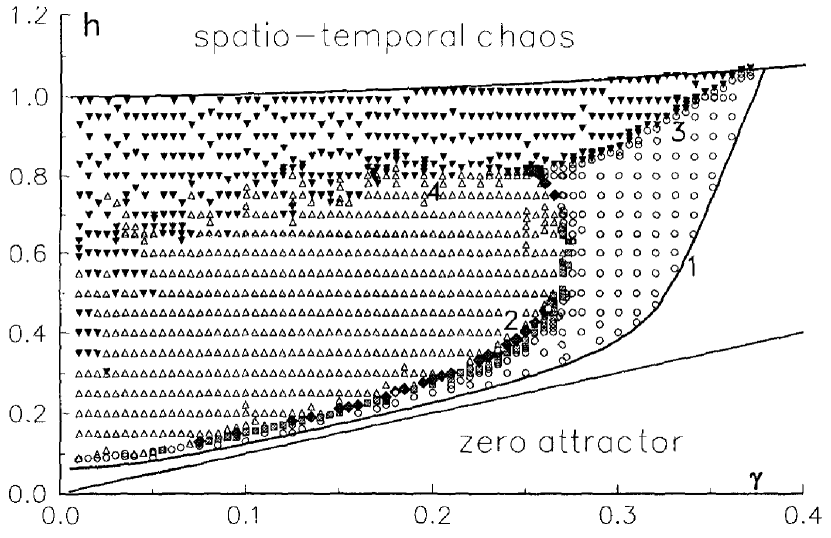
Figure 1: The single-soliton attractor chart for equation (1) compiled by direct numerical simulations Bondila . Stationary solitons serve as attractors in the blank area above the $h=\gamma$ line. The area where only the trivial attractor is available is marked by the empty triangles. Empty circles indicate stable periodic solitons; the black triangles label spatio-temporal chaos. Other symbols mark stable higher-periodic and temporally chaotic solitons. For details see Bondila .

In a short intermediate range of $\gamma$-values, $0.25<\gamma<0.275$, we have a combination of the above two scenarios. The increase of $h$ for the fixed $\gamma$ results in the period-doubling of the soliton, culminating in the temporal-chaotic regime, which is followed by the soliton death. As we continue to raise $h$, an inverse sequence of bifurcations is observed which brings the stable single-periodic soliton back. On further increase of $h$, it loses its stability to a spatio-temporal chaotic state Bondila .

The attractors arising for various $h$ and $\gamma$ values are illustrated by Fig.1 which we reproduce from Ref.Bondila . We should emphasise that this attractor chart has been compiled using direct numerical simulations of equation (1), with a particular choice of initial conditions. (The initial condition was chosen in the form of the unstable soliton $\psi_{+}$ — in the parameter range where it is unstable.) It is an open question, therefore, how robust this chart is. Would it change if simulations started with a different initial condition, or if one used a numerical scheme with different parameters (such as the spatial interval length, the number of the Fourier modes, the full time of simulation, temporal stepsize, etc)? In particular, would qualitative features of the chart survive, e.g. the coexistence of two transformation scenarios, appearance of the desert region, and the peculiar shape of the periodic-attractor domain? One of the aims of the present work is to answer these questions.

III Periodic solitons as solutions of a boundary-value problem in 2D

Instead of solving equation (1) with some initial condition and determining the resulting attractor by running the computation for a sufficiently long time, we were searching for periodic solutions by solving Eq.(1) as a boundary-value problem on a two-dimensional domain $(-\infty,\infty)\times(0,T)$. The boundary conditions were set as

$$\psi(x,t)\to 0\quad\text{as}\ x\to\pm\infty,$$ (4)

and

$$\psi(x,t+T)=\psi(x,t).$$ (5)

The value of $T$ was not available beforehand; the period was regarded as an unknown, together with the solution $\psi(x,t)$.

The periodic solutions were continued (path-followed) in $h$ for the fixed $\gamma$. We employed a predictor-corrector continuation algorithm continuation with a fourth-order Newtonian iteration at each $h$. A finite-difference discretization with the stepsize $\Delta x=0.05$ was used on the interval $(-L,L)=(-50,50)$.

IV Stability of periodic solutions

IV.1 Floquet multipliers

Let $\psi_{0}(x,t)={\cal R}(x,t)+i{\cal I}(x,t)$ be a spatially localised, time-periodic solution. Letting $\psi(x,t)=\psi_{0}(x,t)+u(x,t)+iv(x,t)$ and linearising (1) in the small perturbation $u+iv$, we obtain

$$J{\bf w}_{t}=({\cal H}-\gamma J){\bf w},$$ (6)

where ${\bf w}={\bf w}(x,t)$ is a two-component column-vector

$${\bf w}=\left(\begin{array}[]{c}u\\ v\end{array}\right),$$

$J$ is a skew-symmetric matrix

$$J=\left(\begin{array}[]{cc}0&-1\\ 1&0\end{array}\right),$$

and $\cal H$ is a hermitian matrix-differential operator

$${\cal H}=\left(\begin{array}[]{cc}-\partial_{x}^{2}+1+h-6{\cal R}^{2}-2{\cal I}^{2}&-4{\cal R}{\cal I}\\ -4{\cal R}{\cal I}&-\partial_{x}^{2}+1-h-2{\cal R}^{2}-6{\cal I}^{2}\end{array}\right).$$ (7)

The solution to Eq.(6) with an initial condition ${\bf w}(x,0)$ can be written, formally, as ${\bf w}(x,t)={\cal M}_{t}{\bf w}(x,0),$ where the evolution operator ${\cal M}_{t}$ acts on (vector-) functions of $x$ but depends, parametrically, on $t$. A fundamental role is played by eigenvalues of the monodromy operator ${\cal M}_{T}$:

$${\cal M}_{T}{\bf y}(x)=\mu{\bf y}(x).$$ (8)

Here ${\cal M}_{T}$ is the evolution operator ${\cal M}_{t}$ evaluated at $t=T$. The eigenvalues $\mu$ are usually referred to as the Floquet multipliers and the exponents $\lambda$, where $\mu=e^{\lambda T},$ as the Floquet exponents. According to the Floquet theory, for each $\lambda$ there is a solution ${\bf w}(x,t)$ such that

$${\bf w}(x,t)=e^{\lambda t}{\bf p}(x,t),$$ (9)

where ${\bf p}(x,t)$ is periodic with the period of the solution $\psi_{0}$: ${\bf p}(x,t+T)={\bf p}(x,t)$ for all $t$.

It is useful to establish the relation between the evolution operator ${\cal M}_{t}$ and symplectic maps. Letting ${\bf w}(x,t)=e^{-\gamma t}{\tilde{\bf w}}(x,t)$, Eq.(6) is cast in the form

$$J{\tilde{\bf w}}_{t}={\cal H}{\tilde{\bf w}}.$$ (10)

Since ${\cal H}$ is hermitian, equation (10) is a hamiltonian system (with a quadratic Hamilton functional). The solution to (10) with an initial condition ${\bf w}(x,0)$ is, therefore,

$${\tilde{\bf w}}(x,t)={\cal S}_{t}{\bf w}(x,0),$$

where ${\cal S}_{t}$ is a symplectic map. Thus the evolution operator ${\cal M}_{t}$ and, in particular, the monodromy operator ${\cal M}_{T}$, are related to symplectic maps: ${\cal M}_{t}=e^{-\gamma t}{\cal S}_{t}$ and

$${\cal M}_{T}=e^{-\gamma T}{\cal S}_{T}.$$ (11)

We will use this relation below, in order to explain symmetries of the set of eigenvalues of the operator ${\cal M}_{T}$.

IV.2 Spectrum structure

Stability properties of stationary solutions are determined by eigenvalues $\lambda$ of the operator $(J^{-1}{\cal H}-\gamma)$. The corresponding Floquet multipliers are given by $e^{\lambda T}$ (where $T$ can be chosen arbitrarily for a stationary solution). Therefore the stability eigenvalues $\lambda$ are nothing but the Floquet exponents. Each of the two stationary solitons $\psi_{+}$ and $\psi_{-}$ has just one zero stability eigenvalue (i.e. just one exponent $\lambda=0$). This zero mode originates from the translation invariance of equation (1) — this is the only continuous symmetry the damped-driven equation has.

At the point of the Hopf bifurcation of a stationary solution (a free-standing soliton $\psi_{+}$ or a stationary bound state of solitons), two complex-conjugate eigenvalues $\lambda,\lambda^{*}$ cross into the ${\rm Re}\lambda>0$ half-plane. Irrespectively of what one takes for the value of $T$ in this case, the corresponding Floquet multipliers $\mu=e^{\lambda T}$ and $\mu^{*}=e^{\lambda^{*}T}$ cross through the unit circle on the complex $\mu$-plane. If we, however, take $T$ to be equal to the period of the periodic solution bifurcating off at this point, i.e., let $T=2\pi/{\rm Im}\,\lambda$, the Floquet multipliers cross through the unit circle exactly at $\mu=1$. Adding the unit multiplier associated with the translation invariance, we conclude that any stationary solution has 3 unit Floquet multipliers at the point of its Hopf bifurcation and, accordingly, the detaching periodic solutions should also have 3 unit multipliers at that point.

As we continue the periodic solution $\psi_{0}(x,t)$ away from the point where it was born, two of the unit Floquet multipliers persist (while the third one moves away along the real axis). These two unit multipliers are associated with the translation invariance in $x$ and periodicity in time, respectively. Indeed, if we substitute $\psi_{0}(x,t)$ back in Eq.(1) and differentiate the resulting identity with respect to $x$ and $t$, we will obtain Eq.(6) with ${\bf w}=\partial_{x}\bm{\psi}_{0}$ and ${\bf w}=\partial_{t}\bm{\psi}_{0}$, respectively, where the two-component vector

$$\bm{\psi}_{0}=\left(\begin{array}[]{c}{\cal R}(x,t)\\ {\cal I}(x,t)\end{array}\right).$$

This means that equation (6) has two periodic solutions and the monodromy operator (8) has two eigenvalues $\mu=1$ with eigenfunctions ${\bf w}=\partial_{x}\bm{\psi}_{0}$ and ${\bf w}=\partial_{t}\bm{\psi}_{0}$, respectively. These two unit eigenvalues will routinely arise in our stability analysis of periodic solutions of Eq.(1).

It is not difficult to show that real eigenvalues of ${\cal M}_{T}$ will always arise in pairs whereas the complex eigenvalues will always come in quadruplets. Indeed, the monodromy operator is related to a symplectic map by the relation (11). Real eigenvalues of symplectic maps are known to come in pairs; if $\nu$ is a real eigenvalue of ${\cal S}_{T}$, then so is $\nu^{-1}$. Complex eigenvalues of ${\cal S}_{T}$ come in quadruplets; if $\nu$ is such an eigenvalue, then so are $\nu^{-1},\nu^{*}$, and $(\nu^{*})^{-1}$ Arnold . The relation (11) implies then that if $\mu$ is a real eigenvalue of the evolution operator ${\cal M}_{T}$, then so is ${\hat{\mu}}$, its inverse with respect to the circle of radius $e^{-\gamma T}$:

$$\mu{\hat{\mu}}=e^{-2\gamma T}.$$

In a similar way, if $\mu$ is a complex eigenvalue of ${\cal M}_{T}$, then $\mu^{*}$, ${\hat{\mu}}$, and ${\hat{\mu}}^{*}$ are eigenvalues as well.

We will be referring to ${\hat{\mu}}$ simply as the mirror image of $\mu$. Out of the two Floquet multipliers $\mu$ and ${\hat{\mu}}$ only one can cross the unit circle whereas its mirror image will always be confined inside a smaller circle of the radius $e^{-\gamma T}$. Consequently, when analysing the motion of multipliers on the complex plane and resulting stability changes, we will be focussing on $\mu$ with moduli greater than $e^{-\gamma T}$ and ignoring those with $|\mu|<e^{-\gamma T}$.

Finally, we discuss the location of the continuous spectrum. As $|x|\to\infty$, the operator $(J^{-1}{\cal H}-\gamma)$ becomes a matrix differential operator with constant coefficients whose spectrum is easily determined. Namely, when $h^{2}<1$, the spectrum consists of all $\lambda$ of the form $\lambda=-\gamma\pm ip$, with $\sqrt{1-h^{2}}\leq p\leq\infty$. The corresponding Floquet multipliers fill in a circle of the radius $e^{-\gamma T}$ on the complex $\mu$-plane. When $h^{2}>1$, the continuous spectrum of $(J^{-1}{\cal H}-\gamma)$ fills the vertical line ${\rm Re}\,\lambda=-\gamma$ and an interval on the real axis, $-\gamma-\sqrt{h^{2}-1}<\lambda<-\gamma+\sqrt{h^{2}-1}$. The corresponding Floquet multipliers fill the circle of the radius $e^{-\gamma T}$ and in addition, an interval on the real axis: $e^{-(\gamma+\sqrt{h^{2}-1})T}<\mu<e^{-(\gamma-\sqrt{h^{2}-1})T}$.

IV.3 Numerical stability analysis: the method

To find out whether equation (6) admits solutions of the form (9) with $\mbox{Re}\lambda>0$, we expand $u(x,t)$ and $v(x,t)$ in the Fourier series on the interval $(-L,L)$. The bulk of our eigenvalue calculations were done with $N=100$ but we went up to $N=250$ when the eigenfunctions have shown variations on a small scale.

V Numerical study

V.1 Strong damping: $\gamma=0.30$ and $\gamma=0.35$

We explored $\gamma=0.30$ and $\gamma=0.35$ as two representative sections of the attractor chart in its right-hand part, where numerical simulations had detected no period-doubling bifurcations. The transformation of the solution as it is continued in $h$ is similar in the two cases; see Fig.2.

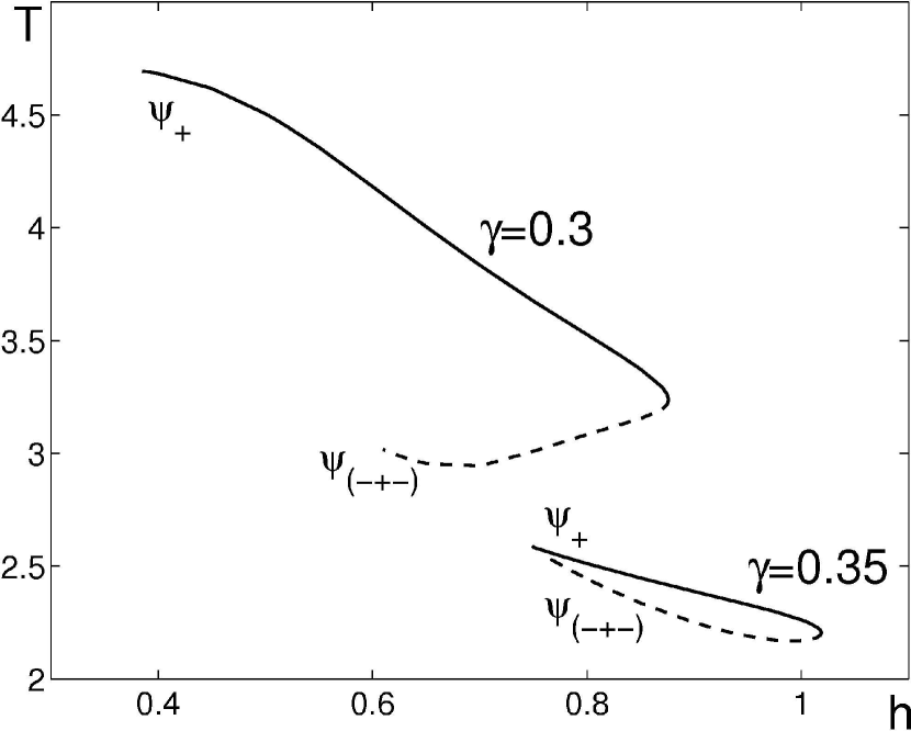
Figure 2: The period of the periodic solutions with $\gamma=0.30$ and $\gamma=0.35$. The solid curves show stable and the dashed ones unstable branches.

The top-end point of each of the two curves in figure 2 corresponds to the stationary single-soliton solution $\psi_{+}$. The underlying value of $h$ equals $0.385$ for $\gamma=0.30$ and $0.7500$ for $\gamma=0.35$. At these $h$, the stationary $\psi_{+}$ soliton undergoes a Hopf bifurcation and a stable periodic solution is born. At the starting point of each curve, the spectrum of the periodic soliton includes three unit multipliers $\mu_{1,2,3}=1$. As $h$ is increased, the eigenvalue $\mu_{3}$ moves inside the unit circle whereas $\mu_{1,2}$ remain at $1$. Meanwhile, five real positive eigenvalues $\mu_{4,...,8}$ detach, one after another, from the continuous spectrum. One of these ($\mu_{8}$) later returns to the continuum while the other four eigenvalues move towards the unit circle. At some point the eigenvalue $\mu_{4}$ collides with $\mu_{3}$ producing a complex pair which, however, later returns to the positive real axis. At the turning point $h_{\rm sn}$, two positive eigenvalues, $\mu_{3}$ and $\mu_{4}$, cross through the unit circle (almost simultaneously). This is where the periodic solution loses its stability. Numerically, the turning-point value is $h_{\rm sn}=0.8761$ for $\gamma=0.30$ and $h_{\rm sn}=1.0186$ for $\gamma=0.35$. On the unstable branch, the spectrum includes two positive eigenvalues $\mu_{3,4}>1$, two unit eigenvalues $\mu_{1,2}=1$, and one positive eigenvalue close to unity ($\mu_{5}<1$). In addition, two more positive eigenvalues approach the unit circle from inside as we continue away from the turning point.

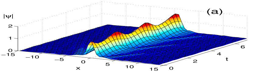
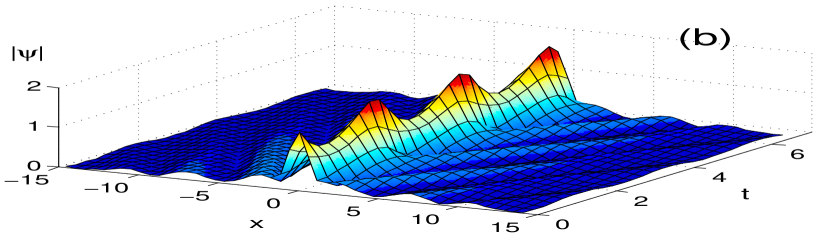
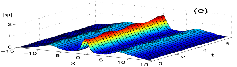
Figure 3: (Color online) The absolute value of the periodic solution with large $\gamma$. In this plot, $\gamma=0.35$. “Motion pictures” (a) and (c) have been taken at the same value of $h$ but correspond to the different branches of the diagram Fig.2: (a) $h=0..85$, $T=2.45$ (top branch) and (c) $h=0.85$, $T=2.34$ (bottom branch). The evolution (b) corresponds to the turning point: $h=1.0185$, $T=2.21$. In each case several periods of oscillation are shown.

It is fitting to note here that the two turning point values, $h_{\rm sn}=0.8761$ and $h_{\rm sn}=1.0186$, are in a good agreement with the boundaries of the periodic-attractor existence domain established previously. Namely, the direct numerical simulation of Eq.(1) gave values close to $0.86$ and $1.01$ for $\gamma=0.30$ and $0.35$, respectively Bondila .

The end point of the dashed curve ($h=0.61$ for $\gamma=0.30$ and $h=0.760$ for $\gamma=0.35$) corresponds to a stationary complex of solitons. In the $\gamma=0.35$ case, this solution has three separate humps in its real and imaginary part. Comparing (the real and imaginary parts of) each of the three humps to (the real and imaginary parts of) the free-standing solitons $\psi_{+}$ and $\psi_{-}$, we conclude that the complex consists of the $\psi_{+}$ soliton in the middle and two solitons $\psi_{-}$ on its sides; that is, the stationary complex should be interpreted as $\psi_{(-+-)}$. The spectrum of discrete eigenvalues of this stationary complex is close to a union of the eigenvalues of the soliton $\psi_{+}$ and those of two solitons $\psi_{-}$. Namely, we have three unit eigenvalues $\mu_{1,2,5}=1$ (resulting from the translation modes of two $\psi_{-}$’s and one $\psi_{+}$) and two eigenvalues $\mu_{6,7}$ close to unity (contributed by the $\psi_{+}$ soliton which is close to its Hopf bifurcation point). In addition, the two $\psi_{-}$ solitons contribute two real positive eigenvalues $\mu_{3,4}>1$.

In the case of $\gamma=0.30$, the two side peaks in the real part of the end-point solution are seen to have merged with the central peak (whose height coincides with the height of the $\psi_{+}$ soliton in its real part). On the other hand, the central peak in the imaginary part of the solution is seen to have disappeared while the two lateral peaks have the same height as the soliton $\psi_{-}$ in its imaginary part. This indicates that the solution can still be interpreted as the $\psi_{(-+-)}$ complex, albeit a tightly bound one.

Representative solutions are shown in figure 3. Near the leftmost point of the curve pertaining to $\gamma=0.35$ in Fig.2, the periodic solution looks like a single soliton with a periodically oscillating amplitude and width [Fig.3(a)]. The soliton is emitting radiation waves; however, the radiation is decaying rapidly as $|x|\to\infty$. As we move further along this curve in Fig.2, the amplitude of oscillations as well as the intensity of radiation increases [Fig.3(b)]. The shape of the oscillating solution evolves into a three-hump structure. Near the end point of the curve, the amplitude of oscillations decreases [Fig.3(c)] and we arrive at the stationary three-soliton complex.

Thus, periodic solitons with large $\gamma$ connect (in the sense of paths in the parameter space) stationary solitons and their complexes, with the connection points provided by the Hopf bifurcations of the latter. It is appropriate to mention a recent publication AW where a similar organisation of the solution manifold was reported for the Benjamin-Ono equation.

V.2 Weak damping: $\gamma=0.1$ and $\gamma=0.2$

Figure 4: The period of the periodic solutions with $\gamma=0.10$ and $\gamma=0.20$. The solid curves show stable and the dashed one unstable branches.

In the weak damping regime we explored two representative values of $\gamma$, $\gamma=0.10$ and $\gamma=0.20$. The two cases exhibit similar bifurcation diagrams (Fig. 4) which are, however, very different from the strong-damping diagrams in Fig.2.

As before, the starting point (the left-end point) of each branch corresponds to the stationary $\psi_{+}$ soliton. At $h=0.1250$ (for $\gamma=0.10$) and $h=0.2275$ (for $\gamma=0.20$) the stationary soliton undergoes a Hopf bifurcation and a periodic solution is born. In Fig.4, this solution is marked $T1$. The spectrum of the $T1$ solution at the starting point of the curve has three unit multipliers, $\mu_{1,2,3}=1$. As $h$ is increased, $\mu_{1}$ moves along the real axis inside the unit circle and immerses in the continuous spectrum at $\mu=e^{-\gamma T}$. For even a larger $h$, a pair of complex-conjugate multipliers with real parts close to $-e^{-\gamma T}$ detaches from the continuum before converging on the negative real axis. One of the resulting real eigenvalues moves towards $-e^{-\gamma T}$ and rejoins the continuum. The other one moves away from the origin and eventually passes through $-1$. This is a signature of the period-doubling bifurcation: the original solution of period $T$ loses its stability and a stable solution with a period $2T$ is born. (This happens at $h_{2T}=0.1463$ and $h_{2T}=0.2663$ for $\gamma=0.10$ and $\gamma=0.20$, respectively.)

The spectrum of the newly born $T2$ solution evolves similarly to the spectrum of $T1$. It is also born with three discrete multipliers $\mu_{1,2,3}=1$. As $h$ increases, $\mu_{1}$ moves along the real axis; immerses in the continuous spectrum; reappears at $-e^{-\gamma T}$, and eventually passes through $-1$ at some $h=h_{4T}$. (The value $h_{4T}$ equals $0.1511$ for $\gamma=0.10$ and $0.2725$ for $\gamma=0.20$.) At this point a new stable branch is born, with the period equal to two periods of $T2$. This new, period-four branch is not shown in Fig. 4.

As for the (unstable) $T1$ solution, the corresponding $T(h)$ curve is snaking up, with the period growing without bound. The solution approaches a homoclinic orbit, connecting the stationary $\psi_{-}$ soliton to itself. In the next subsection, we will discuss this phenomenon in more detail.

We note that the bifurcation diagrams of Fig. 4 are in agreement with direct numerical simulations of Eq.(1) with $\gamma=0.10$ and $\gamma=0.20$ Bondila that revealed the period-doubling transition to temporal chaos in soliton’s dynamics. It is therefore natural to expect that our $T4$ branch will also undergo a period-doubling bifurcation after a short interval of stability, and similarly the branches that it births would undergo a sequence of period-doubling bifurcations. We did not have computational capacity to verify this using our two-dimensional continuation approach. It is worth mentioning, however, that the values of $h$ at which higher-periodic and temporally-chaotic attractors were observed in simulations ($0.16$ and $0.28$ for $\gamma=0.1$ and $0.2$, respectively Bondila ) are close to the $h_{4T}$ given above.

Finally, we have not been able to perform an accurate numerical continuation of solutions with $\gamma=0.05$ and smaller. In this case the solution consists of a finite-extent soliton riding on a (second-harmonic) oscillatory background of a non-negligible amplitude, which shows only a very slow spatial decay as $|x|\to\infty$. [Fig.3(b) gives an idea of the shape of the solution in that case, for most $h$.] In order to obtain this solution under the boundary conditions $\psi(\pm L,t)=0$, one has to enlarge the length of the spatial side of the domain of computation, $(-L,L)\times(0,T)$. This quickly saturates the computational capacity available.

V.3 Intermediate damping: $\gamma=0.265$.

Finally, we investigate the transformation of the periodic solutions with $\gamma$ lying between the strong- and weak-damping ranges. As a representative value of such “borderline” damping, we take $\gamma=0.265$. According to the numerical simulations, the direct period-doubling cascade is followed by an inverse cascade here, resulting in a peculiar shape of the periodicity region on the ($\gamma,h$) plane (Fig.1). Our aim is to provide an explanation for this phenomenon on the basis of the transformations of the periodic solutions as $h$ is continuously varied.

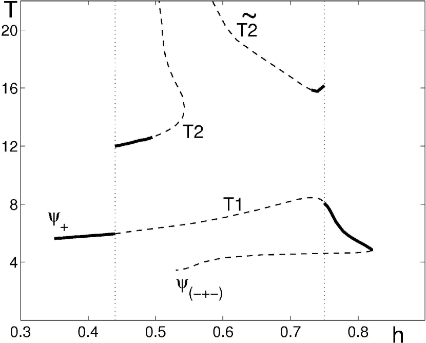
Figure 5: The period of the periodic solution for $\gamma=0.265$. Solid curves show stable and the dashed ones unstable branches.

The results of our numerical continuation are summarised in Fig.5. The bifurcation diagram consists of three branches, the second and third of which arise as a result of the period-doubling bifurcation of the solution on the first branch. The transformation of the solution as we move along this period-one branch [the bottom branch in Fig.5, denoted $T1$] is similar to the transformation of the solution along the curves shown in Fig.2. The starting point of the curve (its leftmost point) corresponds to the stationary solution $\psi_{+}$; the end point corresponds to the stationary complex $\psi_{(-+-)}$. The major difference from the case of large $\gamma$ ($\gamma=0.3$ and $\gamma=0.35$) occurs when a real eigenvalue crosses through $-1$ as $h$ is increased through $h=0.44$. As $h$ is increased past $0.44$, this negative eigenvalue continues to grow in absolute value, reaches a maximum, and then starts to decrease. As $h$ is increased through $h=0.75$, the negative eigenvalue crosses through $-1$ once again, this time in the direction of decreasing modulus. The described behaviour of the negative eigenvalue corresponds to period-doubling bifurcations at $h=0.44$ and $h=0.75$, where periodic solutions with double period are detached. For larger $h$ the solution is stable — all the way to the turning point, where two real eigenvalues cross out through the unit circle.

The spectrum of the first double-periodic solution (detaching at $h=0.44$ and denoted $T2$ in Fig.5) includes two unit eigenvalues, $\mu_{1,2}=1$. When $h=0.44$, there is also a negative eigenvalue $\mu_{3}=-1$. As $h$ is increased from $0.44$, $\mu_{3}$ moves inside the unit circle, then reverses and crosses through $-1$ once again (at $h_{4T}=0.495$). At this point, a new periodic solution $T4$ is born, with the period equal to double the period of the solution $T2$ — roughly four times the period of $T1$. (This “period-four” solution is not shown in Fig.5.) The value $h_{4T}=0.495$ coincides with the largest value of $h$ at which higher-periodic attractors were seen in simulations Bondila .

Returning to the $T2$ solution, it has two positive eigenvalues $\mu_{4,5}$ in addition to the eigenvalues $\mu_{1,2,3}$. As the $T2$ curve in Fig.5 is traced around the turning point at $h=0.543$, these two eigenvalues cross, almost simultaneously, through the unit circle so that $\mu_{4,5}>1$ on the upper branch of the curve. As we continue further along the upper branch, the period of the solution grows: the solution develops a long epoch where it remains very close to the stationary soliton $\psi_{-}$. Each period now consists of two phases: the solution performs a rapid oscillation with its spatio-temporal profile close to that of the $T1$ solution, followed by a slow passage through the bottleneck near the $\psi_{-}$ soliton [see Fig.6].

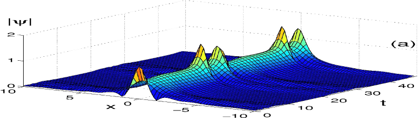
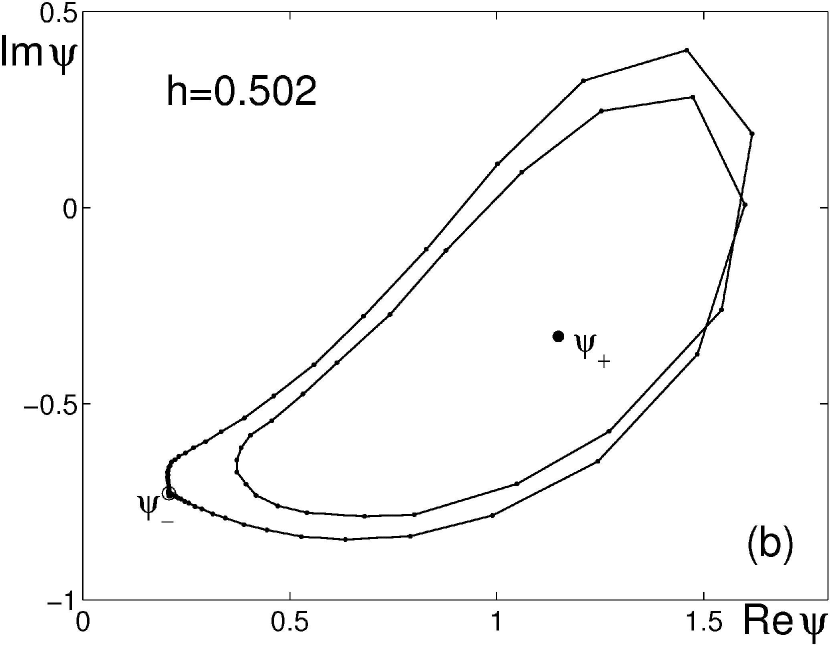
Figure 6: (Color online) (a) The absolute value of the double-periodic solution found on the left upper branch in Fig.5. Here $\gamma=0.265$, $h=0.502$ and $T=22.985$. A rapid oscillation is followed by a long quasistationary epoch where the solution remains close to the $\psi_{-}$ soliton. (b) The phase portrait of this solution taken at $x=0$. Shown is ${\rm Im}\,\psi(0,t)$ vs ${\rm Re}\,\psi(0,t)$. The filled and open circle represent two fixed points: the stationary solitons $\psi_{+}$ and $\psi_{-}$.

The second period-2 solution (denoted $\widetilde{T2}$ in Fig.5), which detaches at $h=0.75$, remains stable for $0.731\leq h\leq 0.75$. As with the first double-periodic solution $T2$, the period of $\widetilde{T2}$ grows as we move along the branch. The solution changes similarly to what we have described in the previous paragraph: a rapid oscillation is followed by a long quasistationary epoch when the solution is very close to the stationary soliton $\psi_{-}$.

Thus, periodic solutions on the $T2$ and $\widetilde{T2}$ branches approach a homoclinic orbit: an infinite-period solution which tends to the stationary soliton $\psi_{-}$ as $t\to-\infty$ and $t\to\infty$. The same transformation scenario was detected in the weak-damping case ($\gamma<0.25$) where the $T1$ (and, presumably, the $T2$) branch was seen to snake up to $T=\infty$ (Fig.4). At the point $h=h_{\infty}$ where the period becomes infinite, the periodic solution undergoes a homocilinic bifurcation which may serve as the source of chaos (see section VII.1 below).

VI Radiation from the oscillating soliton

VI.1 The long-range radiation indicator

Like their stationary counterparts, the oscillatory solitons strike the balance between the energy fed by the driver and the energy lost to the dissipation. This can be quantified, for example, by considering the integral $N=\int_{-R}^{R}|\psi|^{2}dx$. [When the nonlinear Schrödinger equation is employed to describe planar stationary waveguides, this integral measures the total power of light captured by the $(-R,R)$ section of the waveguide. There are energy-related interpretations of this integral in other contexts as well.]

Equation (1) yields

$${\dot{N}}=2h\int_{-R}^{R}\left.|\psi|^{2}\sin(2\theta)dx-2\gamma N+\Phi\right|^{R}_{-R},$$ (12)

where we have decomposed $\psi$ as $|\psi|e^{-i\theta}$ and defined

$$\Phi(x)=i(\psi_{x}\psi^{*}-\psi_{x}^{*}\psi).$$ (13)

The first term in the right-hand side of (12) gives the rate at which the energy is pumped into the soliton while the second one quantifies the damping rate. Assuming that the interval $(-R,R)$ is large enough to contain the core of the soliton, the last term in (13) measures the radiation flux through its endpoints.

The radiation through the points $x=\pm R$ outside the soliton’s core is governed by the linearisation of (1) whose dispersion relation is

$$(\omega-i\gamma)^{2}=(k^{2}+1)^{2}-h^{2}.$$ (14)

The radiation waves emanate from the oscillating soliton which plays the role of a pacemaker for these waves. The pacemaker has a a period $T$ and will sustain waves with frequencies $\omega=2\pi n/T$ ($n=1,2,...$); hence $\omega$ should be taken real in (14). For real $\omega$, equation (14) has two pairs of complex roots $k=\pm(p_{1,2}+iq_{1,2})$, with the imaginary components

$$q_{1,2}=\sqrt{\frac{1}{2}\pm\frac{{\cal S}}{2}+\frac{1}{2}\sqrt{1+2({\cal Q}\pm{\cal S})}},$$ (15)

where

$${\cal S}=\sqrt{{\cal P}+{\cal Q}},\quad{\cal Q}=\sqrt{{\cal P}^{2}+\gamma^{2}\omega^{2}},$$

and $2{\cal P}=h^{2}-\gamma^{2}+\omega^{2}$.

The decay rate $q_{1}$ is always greater than $q_{2}$ and bounded from below ($q_{1}>1$); it accounts for rapidly decaying core of the soliton. Outside the core, the decay rate crosses over to $q_{2}$, and if $q_{2}$ is small the solution enters the long oscillatory wing decaying in proportion to $e^{-q_{2}|x|}$. Periodic solutions that we have reported in this paper all have $\omega\sim 1$; for these, the exponent $q_{2}$ can be small only if $\gamma$ is small.

Assuming that $\gamma$ is small, the expression (15) simplifies. Defining the quantity

$$\sigma=\sigma(\omega)=\sqrt{\omega^{2}+h^{2}-\gamma^{2}}-1,$$ (16)

we have, in particular,

$$q_{2}\to\frac{\omega/2}{1+\sigma}\left(\frac{\gamma}{\sigma}\right)^{1/2}\gamma^{1/2}\quad \text{as}\ \frac{\gamma}{\sigma}\to 0\ (\sigma>0);$$ (17a)

$$q_{2}\to\sqrt{\frac{\omega/2}{1+\sigma}}\,\gamma^{1/2}\quad \text{as}\ \frac{\sigma}{\gamma}\to 0;$$ (17b)

$$q_{2}\to(-\sigma)^{1/2}\quad \text{as}\ \frac{\gamma}{\sigma}\to 0\ (\sigma<0).$$ (17c)

Thus $q_{2}$ is small if $\gamma$ is small while $\sigma$ is positive. In particular, if $\sigma$ is much greater than $\gamma$, the exponent $q_{2}\sim\gamma/\sqrt{\sigma}$ while if $\sigma$ is much smaller than $\gamma$, we have $q_{2}\sim\sqrt{\gamma}$. The decay rate stays small ($\sim\sqrt{-\sigma}$) when $\sigma$ becomes negative — as long as it remains much smaller than $\gamma$ in absolute value. However, as $\sigma$ grows to larger negative values, the exponent $q_{2}$ grows as well. Hence the quantity $\sigma(\omega)$ serves as an indicator of whether the long-range radiation with the frequency $\omega$ can be excited (i.e. whether $q_{2}$ is small) or not.

VI.2 Radiation frequency selection

The harmonic-wave solution of the linearised equation with the decay rate $q_{2}$ is

$$\psi=\eta\left(\cos\phi+i\frac{\alpha\sin\phi-\beta\cos\phi}{({\cal S}+h)^{2}+{\cal T}^{2}}\right)e^{q_{2}x},$$ (18)

where the phase $\phi=\omega t-p_{2}x$, the wavenumber $p_{2}=-{\cal T}/(2q_{2})$, and the coefficients

$$\alpha=\omega({\cal S}+h)+\gamma{\cal T},\quad\beta=\gamma({\cal S}+h)-\omega{\cal T},$$

and ${\cal T}=\sqrt{{\cal Q}-{\cal P}}$. The amplitude $\eta=\eta(\omega)$ is arbitrary as far as the linearised equation is concerned but acquires a specific value when (18) is used to represent radiation from the soliton.

If $R$ is large enough, the solution $\psi(x,t)$ with $x$ near $\pm R$ is described by (18). Substituting (18) in (13) we obtain the flux through the points $x=\pm R$:

$$\Phi(\pm R)=\mp|\eta|^{2}\frac{\cal T}{q_{2}}\,\frac{\omega({\cal S}+h)+\gamma{\cal T}}{({\cal S}+h)^{2}+{\cal T}^{2}}\,e^{-2q_{2}R}.$$ (19)

Assume, first, that $q_{2}$ is of order $1$; this occurs, in particular, when $\gamma\sim 1$. Since $R$ is chosen to be large, the flux through the points $x=\pm R$ in this case is exponentially small: strongly damped radiation waves decay so quickly that they do not reach beyond the core of the soliton (and essentially form part of it). The exponential factor in (19) is not exponentially small only if $q_{2}$ is small; this, in turn, may only happen when the damping is weak.

These considerations have a simple physical interpretation. When $\gamma$ is large, the soliton dissipates most of its excess energy within its core; this is accounted for by the second term in (12). On the other hand, when $\gamma$ is small, the dissipation within the core is insufficient to balance the first term in (12). The long-range radiation may provide an alternative energy-draining mechanism in this case, but this is only available when $q_{2}$ is small which, in turn, is indicated by $\sigma>0$.

If the period of the solution is small enough for the quantity $\sigma(2\pi/T)$ to be positive and much greater than $\gamma$ (which is assumed small), the decay rate $q_{2}$ is close to zero. Therefore, the flux (19) is not exponentially small and the first-harmonic radiation is not blocked in this case. As $T$ is increased so that $h^{2}-\gamma^{2}+(2\pi/T)^{2}$ drops below 1, the decay rate $q_{2}$ grows to values of order $1$. According to eq.(19), the first-harmonic radiation will be mostly suppressed in this case (i.e. damped outside a small neighbourhood of the soliton’s core). However, $\sigma(\omega)$ with $\omega=4\pi/T$ will be still positive; this means that the tails will be dominated by the second-harmonic radiation now. Once the second harmonic is suppressed, the third harmonic will take over, and so on.

We note that the second-harmonic radiation is present not only when the first-harmonic radiation is suppressed. However, the amplitude $\eta(2\pi n/T)$ typically scales as $\epsilon^{n}$ and so Eq.(19) implies that the second-harmonic flux is much weaker than the first-harmonic flux in situations where both channels are open.

VI.3 First-harmonic radiation as a stabilising agent

We routinely calculated the indicator $\sigma(2\pi/T)$ as we continued our periodic solitons. The frequency spectrum of the radiation shows a remarkable correlation with the type of transition the soliton is suffering.

The indicator (16) with $\omega=2\pi/T$ is positive along each curve in Fig.2 — moreover, $\sigma(\omega)$ is much greater than $\gamma$. Therefore, in the case $\gamma>0.275$, the long-range radiation from the soliton is dominated by the first harmonic. On the other hand, $\sigma(2\pi/T)$ is negative along each $T1$ branch in Fig.4 which implies that the first-harmonic radiation is short-range when $\gamma$ is smaller than $0.25$. (When $\gamma=0.10$, $\sigma$ decreases from values close to $-\gamma$ to about $-6\gamma$ along the curve; when $\gamma=0.20$, $\sigma$ drops from zero to nearly $-2.5\gamma$.) In the latter case ($\gamma=0.10$ and $0.20$) the indicator $\sigma(\omega)$ becomes positive if one lets $\omega=4\pi/T$; hence the radiation is second-harmonic here (except for very large $T$ where it is third-harmonic).

This observation allows us to understand, in qualitative terms, why the transformation of the soliton with $\gamma>0.275$ is different from the scenario realised for very weak dampings ($\gamma<0.25$). When $\gamma$ is not very small, the soliton can dispose the excess energy via two channels. Some energy will be lost to the damping in the core region, where $|\psi|\sim 1$ and the term $i\gamma\psi$ is $\sim\gamma$. The rest will be sent away in the form of the strong first-harmonic radiation. Due to the availability of this powerful back-up dissipation channel, the soliton behaves as an overdamped system; hence its enhanced stability. On the other hand, when $\gamma$ is very small, the dominant long-range radiation is second harmonic. Since the amplitude of the $n$-th harmonic radiation scales as $\epsilon^{n}$ where $\epsilon$ is the scale of the amplitude of the oscillation in the core, the second-harmonic radiation is much weaker than the first-harmonic one, and the radiation channel is effectively blocked. The soliton shows the volatility of an underdamped system; hence its instability and period doublings.

The formation of three-soliton complexes observed in the continuation of the oscillatory solitons with $\gamma=0.30$ and $\gamma=0.35$ is also made possible due to the availability of strong radiation with the period equal to the period of the central soliton. The lateral humps in the complex are seeded by the two maxima of the radiation sinusoid which are closest to the central soliton. On the other hand, the second-harmonic radiation available in the $\gamma=0.10$ and $\gamma=0.20$ cases is unable to seed the lateral solitons because it is weak and has the period different from the period of the central hump.

It is interesting to test these qualitative considerations using the case of the intermediate damping, $\gamma=0.265$. In this case the first-harmonic indicator $\sigma(2\pi/T)$ is positive but $\sigma/\gamma$ is not much greater than 1 over the most of the top $T1$ branch in Fig.5. (As $h$ grows from $0.35$ to $0.71$ to $0.78$, the quotient $\sigma/\gamma$ on the top branch changes from $0.5$ to $0$ to $1.$). Accordingly, the first harmonic is strongly damped ($q_{2}\sim\sqrt{\gamma}$) and the long-range radiation is second harmonic. As a result, the soliton suffers period-doubling bifurcations, as in the case of $\gamma=0.10$ and $0.20$. However, as we continue further, the quotient $\sigma/\gamma$ grows (to $2.$ at $h=0.82$) and the first-harmonic radiation takes over from the second-harmonic. Consequently, the solution transforms into a three-soliton complex — as in the case of $\gamma=0.30$ and $0.35$).

VII Discussion and conclusions

VII.1 Homoclinic explosion

The numerical continuation of the T1 solution with $\gamma<0.25$ shows an unbounded growth of its period. The same is true for the T2 solution with $\gamma<0.275$. These observations imply the presence of a homoclinic bifurcation where the period becomes infinite. We now argue that this bifurcation is a source of chaos.

We use results of Shilnikov Shilnikov_1 who considered a three-dimensional dynamical system with a homoclinic orbit connecting a saddle-focus to itself. The saddle-focus is a fixed point with a real unstable eigenvalue $\lambda_{1}>0$ and two complex-conjugate stable eigenvalues $\lambda_{2}=\lambda_{3}^{*}$, ${\rm Re\/}\,\lambda_{2,3}<0$. Assuming that

$$\lambda_{1}>|{\rm Re\/}\,\lambda_{2,3}|,$$ (20)

Shilnikov proved that at the bifurcation point, the system has infinitely many Smale’s horseshoes in a neighbourhood of the homoclinic orbit Shilnikov_1 (see also Shilnikov_2 ). Each of these horseshoes contains an invariant Cantor set with a countable infinity of (unstable) periodic orbits and an uncountable infinity of (unstable) bounded aperiodic orbits — the strange invariant set which manifests itself as attractive or transient chaos. Later it was shown that finitely many of the horseshoes persist on one side of the homoclinic bifurcation GG . The homoclinic bifurcation giving birth to this plethora of periodic and chaotic orbits has been referred to as the “homoclinic explosion” Sparrow .

The homoclinic explosion may also occur in four- and higher-dimensional systems with a homoclinic orbit. The necessary conditions for this are formulated in terms of the eigenvalues of the linearisation about the fixed point connected to itself by the orbit: (a) out of all eigenvalues in the right half of the complex plane, the closest to the imaginary axis is a real eigenvalue $\lambda_{1}$; (b) in the left half of the complex plane, a pair of complex-conjugate eigenvalues $\lambda_{2,3}$ are the closest eigenvalues to the imaginary axis. The homoclinic explosion occurs then if the Shilnikov inequality (20) is satisfied Shilnikov_2 . A carefully studied and clearly explained example of homoclinic explosion in partial differential equations is in Knobloch .

The role of the saddle-focus fixed point in our equation (1) is played by the soliton $\psi_{-}$, Eq.(2). The linear spectrum of this fixed point consists of two discrete eigenvalues, Eqs.(30) of the Appendix, and a continuum of values $\lambda=-\gamma+i\omega$, where $|\omega|\geq\omega_{0}$, $\omega_{0}=\sqrt{1-h^{2}}$. In the left half of the complex plane, the eigenvalue $\lambda_{2}$ is further away from the imaginary axis than the continuous spectrum; hence the dynamics near the saddle-focus will be dominated by the single positive eigenvalue $\lambda_{1}$ and the continuum of eigenvalues with negative real part. This is not exactly the situation of Shilnikov; however it is similar in the sense that the fixed point has a one-dimensional unstable manifold and a more-than-one-dimensional stable manifold, formed by orbits spiralling into the focus. It is natural to expect Shilnikov’s result to remain valid in this case, provided an analog of the inequality (20) is in place — although we do not have any rigorous proof of that. The analog of the Shilnikov inequality in our case is

$$\lambda_{1}>\gamma,$$ (21)

with $\lambda_{1}$ as in (30).

The inequality (21) translates into $(A_{-}^{2}/\sqrt{3})\Lambda_{0}>\gamma$, where $\Lambda_{0}(\epsilon)$ is the positive eigenvalue of the problem (26). One can easily demarcate the region where this inequality is valid. From (25) we have

$$h=\sqrt{\left(\frac{\epsilon}{2+\epsilon}\right)^{2}+\gamma^{2}}.$$ (22)

Equation (22) together with

$$\gamma=\frac{A_{-}^{2}}{\sqrt{3}}\Lambda_{0}(\epsilon)$$ (23)

define the parametric curve $h=h_{\rm Sh}(\gamma)$ on the $(\gamma,h)$ plane. The curve is parabolic in shape (see the dotted curve in the main frame and inset in fig.7); it connects the origin to the point $\gamma=0$, $h=1$. The inequality (21) is valid in the region bounded by this curve and the $h$-axis. This region obviously includes the loci of the homoclinic bifurcations for all $\gamma<0.275$ (see fig.7). Therefore the homoclinic bifurcation is indeed of the homoclinic-explosion type in our case. It is this bifurcation that is responsible for the appearance of temporally chaotic solitons in the parametrically driven damped nonlinear Schrödinger equation.

VII.2 Attractor charts

1. Our analysis answers a number of questions raised by the attractor chart Bondila compiled via direct numerical simulations. One such question concerns the existence of two types of the transformation scenario of the parametrically driven soliton, as the driving strength is raised for the fixed damping coefficient. Is the transformation followed by the soliton with large $\gamma>0.275$ really different from the transition to chaos suffered by its weakly damped counterpart ($\gamma<0.25$), or is this difference caused merely by numerical approximations?

The answer to this question is provided by diagrams in Figs. 2, 4, and 5. In the region $\gamma<0.25$ (represented by the values $\gamma=0.10$ and $0.20$, Fig.4) the increase of $h$ results in a sequence of period-doubling bifurcations of the periodic soliton. On the contrary, no period-doubling bifurcations occur as $h$ is increased for the fixed $\gamma>0.275$. (See Fig.2 showing the diagrams for $\gamma=0.30$ and $0.35$).

2. Another question is why no periodic solitons are observed in numerical simulations with sufficiently large $h$. Is there a well-defined boundary of the domain of existence of stable periodic solitons? We have shown that for $\gamma>0.275$, the region of existence of periodic solitons on the $h$ axis is bounded by the saddle-node bifurcation. No such solutions, stable or unstable, exist above this turning point. For small $\gamma$, $\gamma<0.25$, the region of existence of periodic solitons is also bounded by a turning point; however, solitons cease to exist as attractors for lower values of $h$. The boundary of the stability domain here is set by a narrow strip of temporally-chaotic solitons.

These conclusions verify and explain the formation of the “desert region” on the $(\gamma,h)$ plane. The positions of the saddle-node bifurcation point for $\gamma>0.275$ and the accumulation point of higher-periodic solutions for $\gamma<0.25$, are in good agreement with the boundary of the desert region detected in simulations Bondila .

3. The third issue clarified by our analysis pertains to the shape of the region on the ($\gamma,h$)-plane where periodic solitons are observed in numerical simulations. The question here is why does the $h(\gamma)$ curve bounding this region fold on itself for $\gamma$ between $0.25$ and $0.275$.

This phenomenon is accounted for by the restabilisation of the periodic soliton as $h$ is increased for $\gamma=0.265$ (Fig.5). We note that the case $\gamma=0.265$ is intermediate between the small- and large-$\gamma$ transformation scenarios: On the one hand, similar to the weakly-damped scenario, the soliton undergoes a period-doubling cascade as $h$ is raised for this $\gamma$ (more precisely, it undergoes two period-doubling cascades). On the other, the domain occupied by the periodic attractor is bounded by a saddle-node bifurcation in this case, as in the strongly-damped situation.

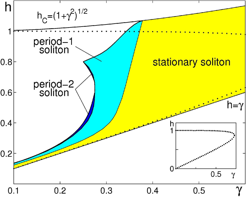
Figure 7: (Color online) Single-soliton attractor chart. The Shilnikov inequality (21) holds inside the region bounded by the dotted curve. The inset gives a wider perspective of this region.

Fig.7 summarises our conclusions on single-soliton periodic attractors. This diagram is in a good agreement with the attractor chart produced using direct numerical simulations, Fig.1.

Appendix A Eigenvalues of the soliton $\psi_{-}$

We let $\psi=\psi_{-}(x)+\delta\psi(x,t)$, where

$$\delta\psi=e^{-i\theta_{-}}[u(x,t)+iv(x,t)]$$

is a small perturbation, and linearise Eq.(1) in $\delta\psi$. Assuming that

$$u(x,t)={\rm Re\/}\left[e^{\lambda t}p(x)\right],\quad v(x,t)={\rm Re\/}\left[e^{\lambda t}q(x)\right]$$

with complex $p$, $q$ and $\lambda$, yields an eigenvalue problem

$$L_{1}p+2{\tilde{\gamma}}q=-{\tilde{\lambda}}q,\quad(L_{0}+\epsilon)q={\tilde{\lambda}}p.$$ (24)

Here we have defined ${\tilde{\gamma}}=\gamma/A_{-}^{2}$ and ${\tilde{\lambda}}=\lambda/A_{-}^{2}$, and introduced two Sturm-Liouville operators with familiar spectral properties:

$$L_{0}=-d^{2}/dX^{2}+1-2\,{\rm sech}^{2}X,$$

$$L_{1}=-d^{2}/dX^{2}+1-6\,{\rm sech}^{2}X.$$

The independent variable $X=A_{-}x$ and the parameter $\epsilon$ was defined by

$$\epsilon=2\sqrt{h^{2}-\gamma^{2}}/A_{-}^{2}.$$ (25)

The two-parameter eigenvalue problem (24) can be reduced BBK to a one-parameter problem

$$L_{1}p=-\Lambda{\tilde{q}},\quad(L_{0}+\epsilon){\tilde{q}}=\Lambda p$$ (26)

by letting

$$\Lambda^{2}=\lambda(\lambda+2{\tilde{\gamma}})$$ (27)

and ${\tilde{q}}=(\lambda+2{\tilde{\gamma}})\lambda^{-1}q$.

The lowest eigenvalue of the operator $L_{0}$ is zero; hence for any $\epsilon>0$ the operator $L_{0}+\epsilon$ is positive definite and the eigenvalue problem (26) can be cast in the form

$$L_{1}p=-\Lambda^{2}Mp,$$ (28)

where $M=(L_{0}+\epsilon)^{-1}$. The operator in the left-hand side is symmetric and the one on the right is symmetric and positive definite; hence all eigenvalues $-\Lambda^{2}$ are real and the function $p(x)$ can also be considered real. The smallest eigenvalue of (28) can be found as a minimum of the Rayleigh quotient:

$$-\Lambda^{2}_{0}=\min_{p\in{\cal L}^{2}}\frac{(p,L_{1}p)}{(p,Mp)},$$ (29)

where $(p,q)$ stands for the ${\cal L}^{2}$ scalar product: $(p,q)=\int p(x)q(x)dx$.

The operator $L_{1}$ has a negative eigenvalue, $\eta_{0}=-3$, with the eigenfunction $y_{0}={\rm sech}^{2}X$. Letting $p=y_{0}$ in Eq.(29), we conclude that the minimum is negative and hence the problem (28) has a negative eigenvalue. We denote the associated eigenfunction $p_{0}(x)$:

$$L_{1}p_{0}=-\Lambda_{0}^{2}Mp_{0}.$$

Since $L_{1}$ does not have any other negative eigenvalues (the only other discrete eigenvalue of $L_{1}$ is $\eta_{1}=0$), the problem (28) does not have any other negative eigenvalues either. Indeed, assume there exist $-\Lambda_{1}^{2}$ and $p_{1}(x)$ such that $L_{1}p_{1}=-\Lambda_{1}^{2}Mp_{1}$. The quadratic form $(y,L_{1}y)$ is then negative definite on the subspace spanned by $p_{0}$ and $p_{1}$; in particular, it is negative for $y(x)=C_{0}p_{0}(x)+C_{1}p_{1}(x)$ where the coefficients are chosen such that $(y,y_{0})=0$. This, however, contradicts the fact that the form $(y,L_{1}y)$ cannot take negative values on the subspace orthogonal to $y_{0}$.

Thus the problem (26) has only one pair of nonzero eigenvalues, $\Lambda_{0}$ and $-\Lambda_{0}$ (where $\Lambda_{0}$ is taken to be positive). The function $\Lambda_{0}(\epsilon)$ has asymptotic behaviours $\Lambda_{0}\to(4\epsilon)^{1/2}$ as $\epsilon\to 0$ and $\Lambda_{0}\to(3\epsilon)^{1/2}$ as $\epsilon\to\infty$; for intermediate values of $\epsilon$ we have tabulated it numerically. Using eq.(27) we recover two eigenvalues of the original, two-parameter, problem (24):

$$\lambda_{1,2}=-\gamma\pm\sqrt{\gamma^{2}+A_{-}^{4}\Lambda_{0}^{2}}.$$ (30)

Here $\lambda_{1}>0$ and $\lambda_{2}<-\gamma<0$.

- (1) J.W. Miles, J. Fluid Mech. 148, 451 (1984)
- (2) E W Laedke and K H Spatschek, J. Fluid Mech.223, 589 (1991)
- (3) C. Elphick and E. Meron, Phys. Rev. A 40, 3226 (1989); X.N. Chen and R.J. Wei, J. Fluid Mech. 259, 291 (1994); W. Zhang and J. Viñals, Phys. Rev. Lett. 74, 690 (1995); A D D Craik and J G M Armitage, Fluid Dyn. Res. 15, 129 (1995); S P Decent and A D D Craik, J, Fluid Mech. 293 237 (1995); W. Wang, X. Wang, J. Wang, and R. Wei, Phys. Lett. A 219, 74 (1996); S P Decent, Fluid Dyn, Res. 21 115 (1997); X. Wang and R. Wei, Phys. Rev. Lett. 78, 2744 (1997); X. Wang and R. Wei, Phys. Rev. E 57, 2405 (1998); G. Miao and R. Wei, Phys. Rev. E 59, 4075 (1999); W Chen, L Lu, Y Zhu, Phys. Rev. E 71, 036622 (2005); L Zhang, X Wang, and Z Tao, Phys. Rev. E 75, 036602 (2007)
- (4) D. Astruc and S. Fauve. In: IUTAM Symposium on Free Surface Flows. Proceedings of the IUTAM Symposium held in Birmingham, UK, 10-14 July 2000. A. C. King and Y. D. Shikhmurzaev, editors. Fluid Mechanics and Its Applications, Vol. 62 (Kluwer, 2001); I V Barashenkov, N V Alexeeva, and E V Zemlyanaya, Phys. Rev. Lett. 89, 104101 (2002)
- (5) M. G. Clerc, S. Coulibaly, and D. Laroze, Phys. Rev. E 77, 056209 (2008); Int. J. of Bifurcation and Chaos, 19, 2717 (2009); ibid. 3525 (2009)
- (6) B. Denardo, B. Galvin, A. Greenfield, A. Larraza, S. Putterman, and W. Wright, Phys. Rev. Lett. 68, 1730 (1992); W.-Z. Chen, Phys. Rev. B 49, 15063 (1994); G. Huang, S.-Y. Lou, and M. Velarde, Int. J. of Bifurcation and Chaos, 6, 1775 (1996); N.V. Alexeeva, I.V. Barashenkov, and G.P. Tsironis, Phys. Rev. Lett. 84, 3053 (2000); W. Chen, B. Hu, H. Zhang, Phys. Rev. B 65, 134302 (2002); H.-Q. Xu and Y. Tang, Chin. Phys. Lett. 23 1544 (2006); J. Cuevas, L. Q. English, P. G. Kevrekidis, and M. Anderson, Phys. Rev. Lett. 102, 224101 (2009)
- (7) I.H. Deutsch and I. Abram, J. Opt. Soc. Am. B 11, 2303 (1994); A. Mecozzi, L. Kath, P. Kumar, and C.G. Goedde, Opt. Lett. 19, 2050 (1994); S. Longhi, Opt. Lett. 20, 695 (1995); V.J. Sánchez-Morcillo, I. Pérez-Arjona, F. Silva, G.J. de Valcárcel, and E. Roldán, Opt. Lett. 25, 957 (2000)
- (8) I.V. Barashenkov, M.M. Bogdan, and V.I. Korobov, Europhys. Lett. 15, 113 (1991)
- (9) M. G. Clerc, S. Coulibaly, D. Laroze, Physica D 239, 72 (2009); Europhys. Lett. 90, 38005 (2010)
- (10) T.-C. Jo and D. Armbruster, Phys. Rev. E 68, 016213 (2003). See also the following references where the parametrically driven cubic Klein-Gordon equation is studied in the Fourier space: W. I. Newman, R. H. Rand, A. L. Newman, Chaos, 9, 242 (1999); T. Bakri, H. G. E. Meijer, F. Verhulst, J. Nonlinear Sci. 19, 571 (2009)
- (11) I V Barashenkov and E V Zemlyanaya, the next submission
- (12) Bondila M, Barashenkov I V, Bogdan M M, Physica D 87 314 (1995)
- (13) N V Alexeeva, I V Barashenkov, and D E Pelinovsky, Nonlinearity 12 103 (1999)
- (14) H Friedel, E W Laedke and K H Spatschek, J. Fluid Mech. 284 341 (1995)
- (15) E.V. Zemlyanaya and I.V. Barashenkov, Math. Modelling 16 3 (2004)
- (16) V. I. Arnold, Mathematical Methods of Classical Mechanics (Graduate Texts in Mathematics). Springer Verlag, New York (2010)
- (17) D M Ambrose and J Wilkening, Commun. Appl. Math. Comput. Sci. 4, 177 (2009); J. Nonlinear Sci. 20, 277 (2010)
- (18) L P Shil’nikov, DAN SSSR 160, 558 (1965)
- (19) L P Shil’nikov, Mat. Sbornik 81 (123), 92 (1970)
- (20) P. Glendinning and C. Sparrow, J. Stat. Phys. 35 645 (1984)
- (21) C. Sparrow, The Lorenz equations: bifurcations, chaos and strange attractors. (Applied Mathematical Sciences 41). Springer-Verlag, New York, 1982
- (22) D. R. Moore, J. Toomre, E. Knobloch and N. O. Weiss. Nature 303, 663 (1983); E. Knobloch, D. R. Moore, J. Toomre, and N. O. Weiss, J. Fluid Mech. 166, 409 (1986)