Decay of helical and non-helical magnetic knots

Abstract

We present calculations of the relaxation of magnetic field structures that have the shape of particular knots and links. A set of helical magnetic flux configurations is considered, which we call $n$-foil knots of which the trefoil knot is the most primitive member. We also consider two nonhelical knots; namely, the Borromean rings as well as a single interlocked flux rope that also serves as the logo of the Inter-University Centre for Astronomy and Astrophysics in Pune, India. The field decay characteristics of both configurations is investigated and compared with previous calculations of helical and nonhelical triple-ring configurations. Unlike earlier nonhelical configurations, the present ones cannot trivially be reduced via flux annihilation to a single ring. For the $n$-foil knots the decay is described by power laws that range form $t^{-2/3}$ to $t^{-1/3}$, which can be as slow as the $t^{-1/3}$ behavior for helical triple-ring structures that were seen in earlier work. The two nonhelical configurations decay like $t^{-1}$, which is somewhat slower than the previously obtained $t^{-3/2}$ behavior in the decay of interlocked rings with zero magnetic helicity. We attribute the difference to the creation of local structures that contain magnetic helicity which inhibits the field decay due to the existence of a lower bound imposed by the realizability condition. We show that net magnetic helicity can be produced resistively as a result of a slight imbalance between mutually canceling helical pieces as they are being driven apart. We speculate that higher order topological invariants beyond magnetic helicity may also be responsible for slowing down the decay of the two more complicated nonhelical structures mentioned above.

I Introduction

Magnetic helicity is an important quantity in dynamo theory FrischPouquet1975 ; BrandenbSubramanianReview2005 , astrophysics RustKumar1996ApJ ; Low1996SoPh and plasma physics Taylor1974 ; Taylor1982 ; JensenChu1984PhFl ; BergerField1984JFM . In the limit of high magnetic Reynolds numbers it is a conserved quantity L.Woltjer061958 . This conservation is responsible for an inverse cascade which can be the cause for large-scale magnetic fields as we observe them in astrophysical objects. The small-scale component of magnetic helicity is responsible for the quenching of dynamo action Gruzinov1994 and has to be shed in order to obtain magnetic fields of equipartition strength and sizes larger then the underlying turbulent eddies BlackmanBrandenburg2003ApJ .

Helical magnetic fields are observed on the Sun’s surface Seehafer1990 ; Pevtsov1995ApJ . Such fields are also produced in tokamak experiments for nuclear fusion to contain the plasma Nelson1995PhPl . It could be shown that the helical structures on the Sun’s surface are more likely to erupt in coronal mass ejections Canfield1999 , which could imply that the Sun sheds magnetic helicity Zhang05 . In Zhang06 it was shown that, for a force-free magnetic field configuration, there exists an upper limit of the magnetic helicity below which the system is in equilibrium. Exceeding this limit leads to coronal mass ejections which drag magnetic helicity from the Sun.

Magnetic helicity is connected with the linking of magnetic field lines. For two separate magnetic flux rings with magnetic flux $\phi_{1}$ and $\phi_{2}$ it can be shown that magnetic helicity is equal to twice the number of mutual linking $n$ times the product of the two fluxes MoffattKnottedness1969 :

$$\mbox{$H_{\rm M}$}=\int_{V}\mathchoice{\mbox{\boldmath$\displaystyle A$}}{\mbox{\boldmath$\textstyle A$}}{\mbox{\boldmath$\scriptstyle A$}}{\mbox{\boldmath$\scriptscriptstyle A$}}{}\cdot\mathchoice{\mbox{\boldmath$\displaystyle B$}}{\mbox{\boldmath$\textstyle B$}}{\mbox{\boldmath$\scriptstyle B$}}{\mbox{\boldmath$\scriptscriptstyle B$}}{}dV=2n\phi_{1}\phi_{2},$$ (1)

where $\textstyle B$ is the magnetic flux density, expressed in terms of the magnetic vector potential $\textstyle A$ via $\mathchoice{\mbox{\boldmath$\displaystyle B$}}{\mbox{\boldmath$\textstyle B$}}{\mbox{\boldmath$\scriptstyle B$}}{\mbox{\boldmath$\scriptscriptstyle B$}}{}=\mathchoice{\mbox{\boldmath$\displaystyle\nabla$}}{\mbox{\boldmath$\textstyle\nabla$}}{\mbox{\boldmath$\scriptstyle\nabla$}}{\mbox{\boldmath$\scriptscriptstyle\nabla$}}{}\times\mathchoice{\mbox{\boldmath$\displaystyle A$}}{\mbox{\boldmath$\textstyle A$}}{\mbox{\boldmath$\scriptstyle A$}}{\mbox{\boldmath$\scriptscriptstyle A$}}{}$ and the integral is taken over the whole volume. As we emphasize in this paper, however, that this formula does not apply to the case of a single interlocked flux tube.

The presence of magnetic helicity constrains the decay of magnetic energy L.Woltjer061958 ; Taylor1974 due to the the realizability condition MoffattBook1978 which imposes a lower bound on the spectral magnetic energy if magnetic helicity is finite; that is,

$$M(k)\geq k|H(k)|/2\mu_{0},$$ (2)

where $M(k)$ and $H(k)$ are magnetic energy and helicity at wave number $k$ and $\mu_{0}$ is the vacuum permeability. These spectra are normalized such that $\int M(k)dk=\langle\mathchoice{\mbox{\boldmath$\displaystyle B$}}{\mbox{\boldmath$\textstyle B$}}{\mbox{\boldmath$\scriptstyle B$}}{\mbox{\boldmath$\scriptscriptstyle B$}}{}^{2}\rangle/2\mu_{0}$ and $\int H(k)dk=\langle\mathchoice{\mbox{\boldmath$\displaystyle A$}}{\mbox{\boldmath$\textstyle A$}}{\mbox{\boldmath$\scriptstyle A$}}{\mbox{\boldmath$\scriptscriptstyle A$}}{}\cdot\mathchoice{\mbox{\boldmath$\displaystyle B$}}{\mbox{\boldmath$\textstyle B$}}{\mbox{\boldmath$\scriptstyle B$}}{\mbox{\boldmath$\scriptscriptstyle B$}}{}\rangle$, where angular brackets denote volume averages. Note that the energy at each scale is bound separately, which constrains conversions from large to small scales and vice versa. For most of our calculations we assume a periodic domain with zero net flux. Otherwise, in the presence of a net flux, magnetic helicity would not be conserved SMG94 ; Ber97 , but it would be produced at a constant rate by the $\alpha$ effect BM04 .

The connection with the topology of the magnetic field makes the magnetic helicity a particularly interesting quantity for studying relaxation processes. One could imagine that the topological structure imposes limits on how magnetic field lines can evolve during magnetic relaxation. To test this it has been studied whether the field topology alone can have an effect on the decay process or if the presence of magnetic helicity is needed fluxRings10 . The outcome was that, even for topologically nontrivial configurations, the decay is only effected by the magnetic helicity content. This was, however, questioned Yeates_Topology_2010 and a topological invariant was introduced via field line mapping which adds another constraint even in absence of magnetic helicity. Further evidence for the importance of extra constraints came from numerical simulations of braided magnetic field with zero magnetic helicity Pontin_etal11 where, at the end of a complex cascade-like process, the system relaxed into an approximately force-free field state consisting of two flux tubes of oppositely signed twist. Since the net magnetic helicity is zero, the evolution of the field would not be governed by Taylor relaxation Taylor1974 but by extra constraints.

A serious shortcoming of some of the earlier work is that the nonhelical field configurations considered so far were still too simple. For example, in the triple ring of fluxRings10 it would have been possible to rearrange freely one of the outer rings on top of the other one without crossing any other field lines. The magnetic flux of these rings would annihilate to zero, making this configuration trivially nonhelical. Therefore, we construct in the present paper more complex nonhelical magnetic field configurations and study the decay of the magnetic field in a similar fashion as in our earlier work. Candidates for suitable field configurations are the IUCAA logo (which is a single nonhelically interlocked flux rope that will be referred to below as the IUCAA knot) and the Borromean rings for which $\mbox{$H_{\rm M}$}=0$. The IUCAA knot is commonly named $8_{18}$ in knot theory. Furthermore, we test if Eq. (1) is applicable for configurations where there are no separated flux tubes while magnetic helicity is finite. Therefore we investigate setups where the magnetic field has the shape of a particular knot which we call $n$–foil knot.

II Model

II.1 Representation of $n$–foil knots

In topology a knot or link can be described via the braid notation ArtinBraids1947 , where the crossings are plotted sequentially, which results in a diagram that resembles a braid. Some convenient starting points have to be chosen from where the lines are drawn in the direction according to the sense of the knot (Figs. 1 and 2)

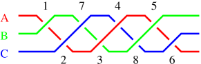
Figure 1: (Color online) Braid representation of the 4–foil knot. The letters denote the starting position and the numbers denote the crossings.

For each crossing either a capital or small letter is assigned depending on whether it is a positive or negative crossing.

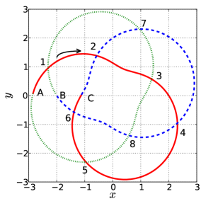
Figure 2: (Color online) $xy$ projection of the 4–foil knot. The numbers denote the crossings while the colors (line styles) separate different parts of the curve. The letters denote the different starting positions for the braid representation in Fig. 1. The arrow shows the sense of the knot.

For the trefoil knot the braid representation is simply AAA. For each new foil a new starting point is needed; at the same time the number of crossings for each line increases by one. This means that, for the 4–foil knot, the braid representation is ABABABAB, for the 5–foil ABCABCABCABCABC, etc.

We construct an initial magnetic field configuration in the form of an $n$–foil knot with $n_{\rm f}$ foils or leaves. First, we construct its spine or backbone as a parametrized curve in three-dimensional space. In analogy to PP_IdealTrefoil_01 we apply the convenient parametrization

$$\mathchoice{\mbox{\boldmath$\displaystyle x$}}{\mbox{\boldmath$\textstyle x$}}{\mbox{\boldmath$\scriptstyle x$}}{\mbox{\boldmath$\scriptscriptstyle x$}}{}(s)=\left(\begin{array}[]{c}(C+\sin{s\mbox{$n_{\rm f}$}})\sin[{s(\mbox{$n_{\rm f}$}-1)}]\\ (C+\sin{s\mbox{$n_{\rm f}$}})\cos[{s(\mbox{$n_{\rm f}$}-1)}]\\ D\cos{s\mbox{$n_{\rm f}$}}\\ \end{array}\right),$$ (3)

where $(C-1)$ is some minimum distance from the origin, $D$ is a stretch factor in the $z$ direction and $s$ is the curve parameter (see Fig. 3).

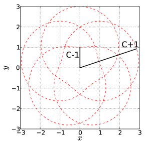
Figure 3: (Color online) Projection of the 5–foil on the $xy$ plane. The lines show the meaning of the distance $C$, which has to be larger than $1$ to make sense.

The strength of the magnetic field across the tube’s cross section is constant and equal to $B_{0}$. In the following we shall use $B_{0}$ as the unit of the magnetic field. Since we do not want the knot to touch itself we set $C=1.6$ and $D=2$. The full three-dimensional magnetic field is constructed radially around this curve (Fig. 4), where the thickness of the cross section is set to $0.48$.

Figure 4: (Color online) Isosurface of the initial magnetic field energy for the 4–foil configuration.

II.2 The IUCAA knot

A prominent example of a single nonhelically interlocked flux rope is the IUCAA knot. For the IUCAA knot we apply a very similar parametrization as for the $n$–foil knots. We have to consider the faster variation in $z$ direction, which yields

$$\mathchoice{\mbox{\boldmath$\displaystyle x$}}{\mbox{\boldmath$\textstyle x$}}{\mbox{\boldmath$\scriptstyle x$}}{\mbox{\boldmath$\scriptscriptstyle x$}}{}(s)=\left(\begin{array}[]{c}(C+\sin{4s})\sin{3s}\\ (C+\sin{4s})\cos{3s}\\ D\cos{(8s-\varphi)}\\ \end{array}\right),$$ (4)

where $C$ and $D$ have the same meaning as for the $n$–foil knots and $\varphi$ is a phase shift of the $z$ variation. The full three-dimensional magnetic field is constructed radially around this curve (Fig. 5), where the thickness of the cross section is set to $0.48$.

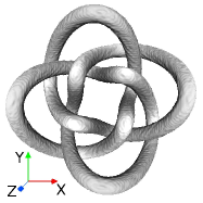
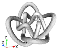
Figure 5: (Color online) Isosurface of the initial magnetic field energy for the IUCAA knot seen from the top (left panel) and slightly from the side (right panel).

II.3 Borromean rings

The Borromean rings are constructed with three ellipses whose surface normals point in the direction of the unit vectors (Fig. 6).

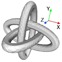
Figure 6: (Color online) Isosurface of the initial magnetic field energy for the Borromean rings configuration.

The major and minor axes are set to $2.5$ and $1$, respectively, and the thickness of the cross section is set to $0.6$. If any one of the three rings were removed, the remaining 2 rings would no longer be interlocked. This means that there is no mutual linking and hence no magnetic helicity. One should, however, not consider this configuration as topologically trivial, since the rings cannot be separated, which is reflected in a nonvanishing third-order topological invariant ruzmaikin:331 .

II.4 Numerical setup

We solve the resistive magnetohydrodynamical (MHD) equations for an isothermal compressible gas, where the gas pressure is given by $p=\rho c_{S}^{2}$, with the density $\rho$ and isothermal sound speed $c_{S}$. Instead of solving for the magnetic field $\textstyle B$ we solve for its vector potential $\textstyle A$ and choose the resistive gauge, since it is numerically well behaved helicityAdvective11 . The equations we solve are

$$\frac{\partial\mathchoice{\mbox{\boldmath$\displaystyle A$}}{\mbox{\boldmath$\textstyle A$}}{\mbox{\boldmath$\scriptstyle A$}}{\mbox{\boldmath$\scriptscriptstyle A$}}{}}{\partial t}=\mathchoice{\mbox{\boldmath$\displaystyle U$}}{\mbox{\boldmath$\textstyle U$}}{\mbox{\boldmath$\scriptstyle U$}}{\mbox{\boldmath$\scriptscriptstyle U$}}{}\times\mathchoice{\mbox{\boldmath$\displaystyle B$}}{\mbox{\boldmath$\textstyle B$}}{\mbox{\boldmath$\scriptstyle B$}}{\mbox{\boldmath$\scriptscriptstyle B$}}{}+\eta\nabla^{2}\mathchoice{\mbox{\boldmath$\displaystyle A$}}{\mbox{\boldmath$\textstyle A$}}{\mbox{\boldmath$\scriptstyle A$}}{\mbox{\boldmath$\scriptscriptstyle A$}}{},$$ (5)

$$\frac{{\rm D}{}\mathchoice{\mbox{\boldmath$\displaystyle U$}}{\mbox{\boldmath$\textstyle U$}}{\mbox{\boldmath$\scriptstyle U$}}{\mbox{\boldmath$\scriptscriptstyle U$}}{}}{{\rm D}{}t}=-c_{\rm S}^{2}\mathchoice{\mbox{\boldmath$\displaystyle\nabla$}}{\mbox{\boldmath$\textstyle\nabla$}}{\mbox{\boldmath$\scriptstyle\nabla$}}{\mbox{\boldmath$\scriptscriptstyle\nabla$}}{}\ln{\rho}+\mathchoice{\mbox{\boldmath$\displaystyle J$}}{\mbox{\boldmath$\textstyle J$}}{\mbox{\boldmath$\scriptstyle J$}}{\mbox{\boldmath$\scriptscriptstyle J$}}{}\times\mathchoice{\mbox{\boldmath$\displaystyle B$}}{\mbox{\boldmath$\textstyle B$}}{\mbox{\boldmath$\scriptstyle B$}}{\mbox{\boldmath$\scriptscriptstyle B$}}{}/\rho+\mathchoice{\mbox{\boldmath$\displaystyle F$}}{\mbox{\boldmath$\textstyle F$}}{\mbox{\boldmath$\scriptstyle F$}}{\mbox{\boldmath$\scriptscriptstyle F$}}{}_{\rm visc},$$ (6)

$$\frac{{\rm D}{}\ln{\rho}}{{\rm D}{}t}=-\mathchoice{\mbox{\boldmath$\displaystyle\nabla$}}{\mbox{\boldmath$\textstyle\nabla$}}{\mbox{\boldmath$\scriptstyle\nabla$}}{\mbox{\boldmath$\scriptscriptstyle\nabla$}}{}\cdot\mathchoice{\mbox{\boldmath$\displaystyle U$}}{\mbox{\boldmath$\textstyle U$}}{\mbox{\boldmath$\scriptstyle U$}}{\mbox{\boldmath$\scriptscriptstyle U$}}{},$$ (7)

where $\textstyle U$ is the velocity field, $\eta$ is the magnetic diffusivity, $\mathchoice{\mbox{\boldmath$\displaystyle J$}}{\mbox{\boldmath$\textstyle J$}}{\mbox{\boldmath$\scriptstyle J$}}{\mbox{\boldmath$\scriptscriptstyle J$}}{}=\mathchoice{\mbox{\boldmath$\displaystyle\nabla$}}{\mbox{\boldmath$\textstyle\nabla$}}{\mbox{\boldmath$\scriptstyle\nabla$}}{\mbox{\boldmath$\scriptscriptstyle\nabla$}}{}\times\mathchoice{\mbox{\boldmath$\displaystyle B$}}{\mbox{\boldmath$\textstyle B$}}{\mbox{\boldmath$\scriptstyle B$}}{\mbox{\boldmath$\scriptscriptstyle B$}}{}/\mu_{0}$ is the current density, $\mathchoice{\mbox{\boldmath$\displaystyle F$}}{\mbox{\boldmath$\textstyle F$}}{\mbox{\boldmath$\scriptstyle F$}}{\mbox{\boldmath$\scriptscriptstyle F$}}{}_{\rm visc}=\rho^{-1}\mathchoice{\mbox{\boldmath$\displaystyle\nabla$}}{\mbox{\boldmath$\textstyle\nabla$}}{\mbox{\boldmath$\scriptstyle\nabla$}}{\mbox{\boldmath$\scriptscriptstyle\nabla$}}{}\cdot 2\nu\rho\bm{\mathsf{S}}$ is the viscous force with the traceless rate of strain tensor $\bm{\mathsf{S}}$ with components ${\sf S}_{ij}=\frac{1}{2}(u_{i,j}+u_{j,i})-\frac{1}{3}\delta_{ij}\mathchoice{\mbox{\boldmath$\displaystyle\nabla$}}{\mbox{\boldmath$\textstyle\nabla$}}{\mbox{\boldmath$\scriptstyle\nabla$}}{\mbox{\boldmath$\scriptscriptstyle\nabla$}}{}\cdot\mathchoice{\mbox{\boldmath$\displaystyle U$}}{\mbox{\boldmath$\textstyle U$}}{\mbox{\boldmath$\scriptstyle U$}}{\mbox{\boldmath$\scriptscriptstyle U$}}{}$, $\nu$ is the kinematic viscosity, and ${\rm D}{}/{\rm D}{}t=\partial/\partial t+\mathchoice{\mbox{\boldmath$\displaystyle U$}}{\mbox{\boldmath$\textstyle U$}}{\mbox{\boldmath$\scriptstyle U$}}{\mbox{\boldmath$\scriptscriptstyle U$}}{}\cdot\nabla$ is the advective time derivative. We perform simulations in a box of size $(2\pi)^{3}$ with fully periodic boundary conditions for all quantities. To test how boundary effects play a role we also perform simulations with perfect conductor boundary conditions (i.e., the component of the magnetic field perpendicular to the surface vanishes). In both choices of boundary conditions, magnetic helicity is gauge invariant and is a conserved quantity in ideal MHD (i.e., $\eta=0$). As a convenient parameter we use the Lundquist number $\mbox{\rm Lu}=U_{\rm A}L/\eta$, where $U_{\rm A}$ is the Alfvén velocity and $L$ is a typical length scale of the system. The value of the viscosity is characterized by the magnetic Prandtl number $\mbox{\rm Pr}_{\rm M}=\nu/\eta$. However, in all cases discussed below we use $\mbox{\rm Pr}_{\rm M}=1$. To facilitate comparison of different setups it is convenient to normalize time by the resistive time $t_{\rm res}=r^{2}\pi/\eta$, where $r$ is the radius of the cross section of the flux tube.

We solve Eqs. (5)–(7) with the Pencil Code BD02PC , which employs sixth-order finite differences in space and a third-order time stepping scheme. As in our earlier work fluxRings10 , we use $256^{3}$ meshpoints for all our calculations. We recall that we use explicit viscosity and magnetic diffusivity. Their values are dominant over numerical contributions associated with discretization errors of the scheme .

III RESULTS

III.1 Helicity of $n$–foil knots

We test equation (1) for the $n$–foil knots in order to see how the number of foils $n_{\rm f}$ relates to the number of mutual linking $n$ for the separated flux tubes. From our simulations we know the magnetic helicity $H_{\rm M}$ and the magnetic flux $\phi$ through the tube. Solving (1) for $n$ will lead to an apparent self-linking number which we call $n_{\rm app}$. It turns out that $n_{\rm app}$ is much larger then $n_{\rm f}$ and increases faster (Fig. 7).

We note that (1) does not apply to this setup of flux tubes and propose therefore a different formula for the magnetic helicity:

$$H_{\rm M} = (\mbox{$n_{\rm f}$}-2)\mbox{$n_{\rm f}$}\phi^{2}/2.$$ (8)

In Fig. 7 we plot the apparent linking number together with a fit which uses equation (8).

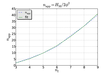
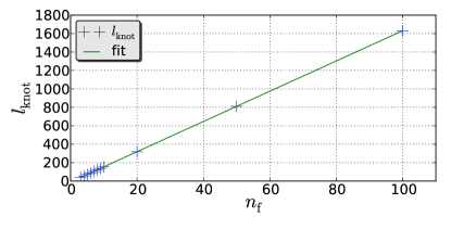
Figure 7: (Color online) The apparent self-linking number for $n$–foil knots with respect to $n_{\rm f}$ (upper panel). The fit is obtained by equating (1) and (8). The length of a $n$–foil knot is plotted with respect to $n_{\rm f}$ (lower panel), which can be fit almost perfectly by a linear function.

Equation (8) can be motivated via the number of crossings. The flux tube is projected onto the $xy$ plane such that the number of crossings is minimal. The linking number can be determined by adding all positive crossings and subtracting all negative crossings according to Fig. 8.

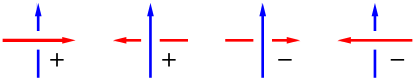
Figure 8: (Color online) Schematic representation illustrating the sign of a crossing. Each crossing has a handedness which can be either positive or negative. The sum of the crossings gives the number of linking and eventually the magnetic helicity content via equation (8).

The linking number is then simply given as SchareinPhD

$$n_{\rm linking}=(n_{+}-n_{-})/2,$$ (9)

where $n_{+}$ and $n_{-}$ correspond to positive and negative crossings, respectively. If we set $n_{\rm linking}=n_{\rm app}$ then we easily see the validation of (8). Each new foil creates a new ring of crossings and adds up one crossing in each ring (see Fig. 9), which explains the quadratic increase.

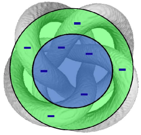
Figure 9: (Color online) The isosurface for the 4–foil knot field configuration. The sign of the crossing is always negative. The rings show the different areas where crossings occur.

III.2 Magnetic energy decay for $n$–foil knots

Next, we plot in Fig. 10 the magnetic energy decay for $n$–foil knots with $\mbox{$n_{\rm f}$}=3$ up to $\mbox{$n_{\rm f}$}=7$ for periodic boundary conditions. It turns out that, at later times, the decay slows down as $n_{\rm f}$ increases. The decay of the magnetic energy obeys an approximate $t^{-2/3}$ law for $\mbox{$n_{\rm f}$}=3$ and a $t^{-1/3}$ law for $\mbox{$n_{\rm f}$}=7$. The rather slow decay is surprising in view of earlier results that, for turbulent magnetic fields, the magnetic energy decays like $t^{-1}$ in the absence of magnetic helicity and like $t^{-1/2}$ with magnetic helicity CHB05 . Whether or not the decay seen in Fig. 10 really does follow a power law with such an exponent remains therefore open.

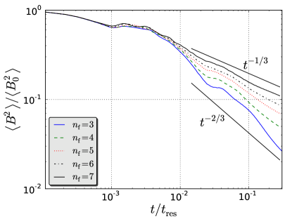
Figure 10: (Color online) Time dependence of the normalized magnetic energy for a given number of foils with periodic boundary conditions. The power law for the energy decay varies between $-2/3$ for $\mbox{$n_{\rm f}$}=3$ (solid/blue line) and $-1/3$ for $\mbox{$n_{\rm f}$}=7$ (solid/black).

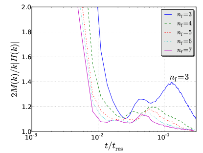
Figure 11: (Color online) Time dependence of the quotient from the realizability condition (2) for $k=2$. It is clear that, for larger $n_{\rm f}$, the energy approaches its minimum faster.

The different power laws for a given number of foils $n_{\rm f}$ are unexpected because the setups differ only in their magnetic helicity and magnetic energy content and not in the qualitative nature of the knot. Indeed, one might have speculated that the faster $t^{-2/3}$ decay applies to the case with larger $n_{\rm f}$, because this structure is more complex and involves sharper gradients. On the other hand, a larger value of $n_{\rm f}$ increases the total helicity, making the resulting knot more strongly packed. This can be verified by noting that the magnetic helicity increases quadratically with $n_{\rm f}$ while the magnetic energy increases only linearly. This is because the energy is proportional to the length of the tube which, in turn, is proportional to $n_{\rm f}$ (Fig. 7). Therefore we expect that, for the higher $n_{\rm f}$ cases, the realizability condition should play a more significant role at early times. This can be seen in Fig. 11, where we plot the ratio $2M(k)/(k|H(k)|)$ for $\mbox{$n_{\rm f}$}=3$ to $\mbox{$n_{\rm f}$}=7$ for $k=2$. Since the magnetic helicity relative to the magnetic energy is higher for larger values of $n_{\rm f}$, it plays a more significant role for high $n_{\rm f}$. This would explain a different onset of the power law decay, although it would not explain a change in the exponent. Indeed the decay of $H_{\rm M}$ shows approximately the same behavior for all $n_{\rm f}$ (Fig. 12). We must therefore expect that the different decay laws are described only approximately by power laws.

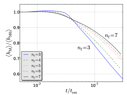
Figure 12: (Color online) Time dependence of the normalized magnetic helicity for a given number of foils with periodic boundary conditions.

For periodic boundary conditions it is possible that the flux tube reconnects over the domain boundaries which could lead to additional magnetic field destruction. To exclude such complications we compare simulations with perfectly conducting or closed boundaries with periodic boundary conditions (Fig.13). Since there is no difference in the two cases we can exclude the significance of boundary effects for the magnetic energy decay.

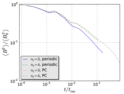
Figure 13: (Color online) Time dependence of the normalized magnetic energy for the trefoil and 4–foil knot with periodic and perfect conductor (PC) boundary conditions. There is no significant difference in the energy decay for the different boundary conditions.

In all cases the magnetic helicity can only decay on a resistive time scale (Fig. 12). This means that, during faster dynamical processes like magnetic reconnection, magnetic helicity is approximately conserved. To show this we plot the magnetic field lines for the trefoil knot at different times (Fig. 14). Since magnetic helicity does not change significantly, the self-linking is transformed into a twisting of the flux tube which is topologically equivalent to linking. Such a process has also been mentioned in connection with Fig. 1 of Ref. PhysRevLett.83.1155 , while the opposite process of the conversion of twist into linkage has been seen in Ref. Linton_etal01 . We can also see that the reconnection process, which transforms the trefoil knot into a twisted ring, does not aid the decay of magnetic helicity.

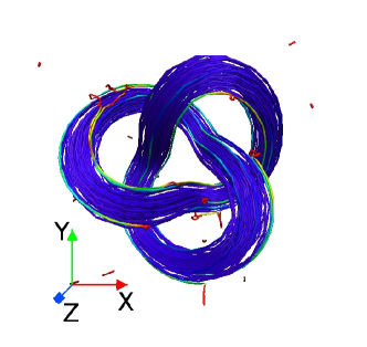
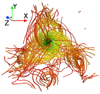
Figure 14: (Color online) Magnetic field lines for the trefoil knot at time $t=0$ (upper panel) and $t=7.76\times 10^{-2}\,t_{\rm res}$ (lower panel). Both images were taken from the same viewing position to make comparisons easier. The Lundquist number was chosen to be $1000$. The colors indicate the field strength.

III.3 Decay of the IUCAA knot

For the nonhelical triple-ring configuration of Ref. fluxRings10 it was found that the topological structure gets destroyed after only $10$ Alfvén times. The destruction was attributed to the absence of magnetic helicity whose conservation would pose constraints on the relaxation process. Looking at the magnetic field lines of the IUCAA knot at different times (Fig. 15), we see that the field remains structured and that some helical features emerge above and below the $z=0$ plane. These localized helical patches could then locally impose constraints on the magnetic field decay.

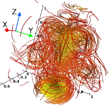
Figure 15: (Color online) Magnetic field lines for the IUCAA knot at $t=0.108\,t_{\rm res}$ (upper panel) and at $t=0.216\,t_{\rm res}$ (lower panel) for $\mbox{\rm Lu}=1000$ and $\varphi=(4/3)\pi$.

The asymmetry of the IUCAA knot in the $z$ direction leads to different signs of magnetic helicity above and below the $z=0$ plane. This is shown in Figs. 16 and 17 where we plot the magnetic helicity for the upper and lower parts for two different values of $\varphi$; see Eq. (4). In the plot, we refer to the upper and lower parts as north and south, respectively. These plots show that there is a tendency of magnetic helicity of opposite sign to emerge above and below the $z=0$ plane. Given that the magnetic helicity was initially zero, one may speculate that higher order topological invariants could provide an appropriate tool to characterize the emergence of such a “bi-helical” structure from an initially nonhelical one.

Figure 16: (Color online) Normalized magnetic helicity in the northern (green/dashed line) and southern (red/dotted line) domain half together with the total magnetic helicity (blue/solid line) for the IUCAA knot with $\mbox{\rm Lu}=2000$ and $\varphi=(4/3)\pi$.

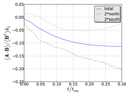
Figure 17: (Color online) Normalized magnetic helicity in the northern (green/dashed line) and southern (red/dotted line) domain half together with the total magnetic helicity (blue/solid line) for the IUCAA knot with $\mbox{\rm Lu}=2000$ and $\varphi=(4/3+0.2)\pi$.

Note that there is a net increase of magnetic helicity over the full volume. Furthermore, the initial magnetic helicity is not exactly zero either, but this is probably a consequence of discretization errors associated with the initialization. The subsequent increase of magnetic helicity can only occur on the longer resistive time scales, since magnetic helicity is conserved on dynamical time scales. Note, however, that the increase of magnetic helicity is exaggerated because we divide by the mean magnetic energy density which is decreasing with time.

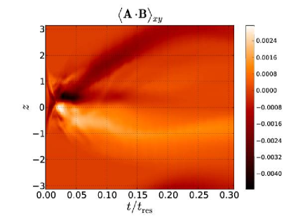
Figure 18: (Color online) $xy$-averaged magnetic helicity density profile in $z$ direction for the IUCAA knot with $\mbox{\rm Lu}=2000$ and $\varphi=(4/3)\pi$. There is an apparent asymmetry in the distribution amongst the hemispheres.

In Fig. 18 we plot the $xy$-averaged magnetic helicity as a function of $z$ and $t$. This shows that the asymmetry between upper and lower parts increases with time, which we attribute to the Lorentz forces through which the knot shrinks and compresses its interior. This is followed by the ejection of magnetic field.

To clarify this we plot slices of the magnetic energy density in the $xz$ plane for different times (Fig. 19). The slices are set in the center of the domain.

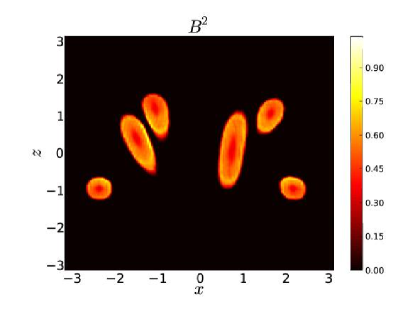
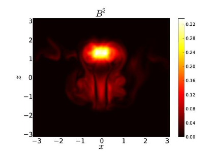
Figure 19: (Color online) Magnetic energy density in the $xz$ plane for $y=0$ at $t=0$ (upper panel) and $t=5.58\times 10^{-2}\,t_{\rm res}$ (lower panel) for the IUCAA knot with $\mbox{\rm Lu}=2000$ and $\varphi=(4/3)\pi$.

Due to the rose-like shape, our representation of the IUCAA knot is not quite symmetric and turns out to be narrower in the lower half (negative $z$) than in the upper half (positive $z$), which is shown in Fig. 5 (right panel). When the knot contracts due to the Lorentz force, it begins to touch the inner parts which creates motions in the positive $z$ direction which, in turn, drag the magnetic field away from the center (Fig. 19). The pushing of material can, however, be decreased when the phase $\varphi$ is changed. For $\varphi=(4/3+0.2)\pi$ there is no such upward motion visible and the configuration stays nearly symmetric (Fig. 20).

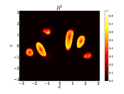
Figure 20: (Color online) Magnetic energy density in the $xz$-plane for $y=0$ at $t=0$ (upper panel) and $t=5.58\times 10^{-2}\,t_{\rm res}$ (lower panel) for the IUCAA knot with $\mbox{\rm Lu}=2000$ and $\varphi=(4/3+0.2)\pi$. The magnetic field stays centered.

In Fig. 21 the decay behavior of the magnetic energy is compared with previous work fluxRings10 . We note in passing that the power law of $t^{-1}$ is expected for nonhelical turbulence CHB05 , but it is different from the helical ($t^{-1/2}$) and nonhelical ($t^{-3/2}$) triple-ring configurations studied earlier. A possible explanation is the conservation of magnetic structures for the IUCAA knot, whereas the nonhelical triple-ring configuration loses its structure.

III.4 Borromean rings

Previous calculations showed a significant difference in the decay process of three interlocked flux rings in the helical and nonhelical case fluxRings10 . In Fig. 21 we compare the magnetic energy decay found from previous calculations using triple-ring configurations with the IUCAA knot and the Borromean rings.

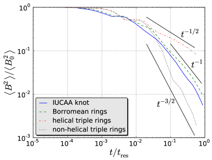
Figure 21: (Color online) Magnetic energy versus time for the different initial field configurations together with power laws which serve as a guide. The decay speed of the IUCAA knot and Borromean rings lies well in between the helical and nonhelical triple-ring configuration.

The Borromean rings show a similar behavior as the IUCAA knot where the magnetic energy decays like $t^{-1}$. Similarly to the IUCAA knot we expect some structure, which is conserved during the relaxation process and causes the relatively slow energy decay compared to other nonhelical configurations. We plot the magnetic field lines at times $t=0.248\,t_{\rm res}$ and $t=0.276\,t_{\rm res}$; see Figs. 22 and 23, respectively. At $t=0.248\,t_{\rm res}$ there are two interlocked flux rings in the lower left corner, while in the opposite half of the simulation domain a clearly twisted flux ring becomes visible. The interlocked rings reconnect at $t=0.276\,t_{\rm res}$ and merge into one flux tube with a twist opposite to the other flux ring. The magnetic helicity stays zero during the reconnection, but changes locally, which then imposes a constraint on the magnetic energy decay and could explain the power law that we see in Fig. 21. This finding is similar to that of Ruzmaikin and Akhmetiev ruzmaikin:331 who propose that, after reconnection, the Borromean ring configuration transforms first into a trefoil knot and three 8-form flux tubes and after subsequent reconnection into two untwisted flux rings (so-called unknots) and six 8-form flux tubes. We can partly reproduce this behavior, but instead of a trefoil knot we obtain two interlocked flux rings and, instead of the 8-form flux tubes, we obtain internal twist in the flux rings.

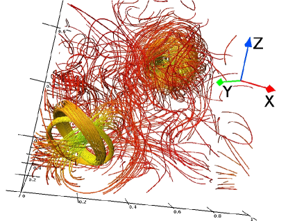
Figure 22: (Color online) Magnetic field lines at $t=0.248\,t_{\rm res}$ for the Borromean rings configuration for $\mbox{\rm Lu}=1000$. In the lower-left corner the interlocked flux rings are clearly visible which differs from the proposed trefoil knot ruzmaikin:331 . The flux ring in the opposite corner has an internal twist which makes it helical. The colors denote the strength of the field, where the scale goes from red over green to blue.

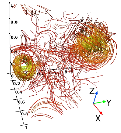
Figure 23: (Color online) Magnetic field lines at $t=0.276\,t_{\rm res}$ for the Borromean rings configuration for $\mbox{\rm Lu}=1000$. The two flux rings in the corners both have an internal twist which makes them helical. The twist is, however, of opposite sign which means that the whole configuration does not contain magnetic helicity. The colors denote the strength of the field, where the scale goes from red over green to blue.

IV Conclusions

In this paper we have analyzed for the first time the decay of complex helical and nonhelical magnetic flux configurations. A particularly remarkable one is the IUCAA knot for which the linking number is zero, and nevertheless, some finite magnetic helicity is gradually emerging from the system on a resistive time scale. It turns out that both the IUCAA knot and the Borromean rings develop regions of opposite magnetic helicity above and below the midplane, so the net magnetic helicity remains approximately zero. In that process, any slight imbalance can then lead to the amplification of the ratio of magnetic helicity to magnetic energy—even though the magnetic field on the whole is decaying. This clearly illustrates the potential of nonhelical configurations to exhibit nontrivial behavior, and thus the need for studying the evolution of higher order invariants that might capture such processes.

The role of resistivity in producing magnetic helicity from a nonhelical initial state has recently been emphasized Low11 , but it remained puzzling how a resistive decay can increase the topological complexity of the field, as measured by the magnetic helicity. Our results now shed some light on this. Indeed, the initial field in our examples has topological complexity that is not captured by the magnetic helicity as a quadratic invariant. This is because of mutual cancellations that can gradually undo themselves during the resistive decay process, leading thus to finite magnetic helicity of opposite sign in spatially separated locations. We recall in this context that the magnetic helicity over the periodic domains considered here is gauge invariant and should thus agree with any other definition, including the absolute helicity defined in Ref. Low11 .

Contrary to our own work on a nonhelical interlocked flux configuration fluxRings10 , which was reducible to a single flux ring after mutual annihilation of two rings, the configurations studied here are non-reducible even when mutual annihilation is taken into account.

For the helical $n$–foil knot, we have shown that the magnetic helicity increases quadratically with $n$. Furthermore, their decay exhibits different power laws of magnetic energy which lie between $t^{-2/3}$ for the 3–foil knot and $t^{-1/3}$ for the 7–foil knot. The latter case corresponds well with the previously discussed case of three interlocked flux rings that are interlocked in a helical fashion. The appearance of different power laws seems surprising since we first expected a uniform power law in all helical cases in the regime where the magnetic helicity is so large that the realizability condition plays a role. This makes us speculate whether there are other quantities that are different for the various knots and constrain magnetic energy decay. Such quantities would be higher order topological invariants ruzmaikin:331 , which are so far only defined for spatially separated flux tubes. In order to investigate their role they need to be generalized such that they can be computed for any magnetic field configuration, similar to the integral for the magnetic helicity.

The power law of $t^{-1}$ in the decay of the magnetic energy for the IUCAA knot and the Borromean rings is different from the $t^{-3/2}$ behavior found earlier for the nonhelical triple-ring configuration. The observed decay rate can be attributed to the creation of local helical structures that constrain the decay of the local magnetic field. But we cannot exclude higher order invariants ruzmaikin:331 whose conservation would then constrain the energy decay.

The Borromean rings showed clearly that local helical structures can be generated without forcing the system. These can then impose constraints on the field decay. We suggest that spatial variations should be taken into account to reformulate the realizability condition (2), which would increase the lower bound for the magnetic energy. For astrophysical systems local magnetic helicity variations have to be considered to give a more precise description of both relaxation and reconnection processes.

Both the IUCAA logo and the Borromean rings do not stay stable during the simulation time and split up into two separated helical magnetic structures. On the other hand we see that the helical $n$–foil knots stay stable. A similar behavior was seen in Braithwaite2010MNRAS , where magnetic fields in bubbles inside galaxy clusters were simulated. In the case of a helical initial magnetic field the field decays into a confined structure, while for sufficiently low initial magnetic helicity, separated structures of opposite magnetic helicity seem more preferable.

- (1) U. Frisch, A. Pouquet, J. Leorat, and A. Mazure, “Possibility of an inverse cascade of magnetic helicity in magnetohydrodynamic turbulence,” J. Fluid Mech., vol. 68, pp. 769–778, 1975.
- (2) A. Brandenburg and K. Subramanian, “Astrophysical magnetic fields and nonlinear dynamo theory,” Phys. Rep., vol. 417, pp. 1–209, 2005.
- (3) D. M. Rust and A. Kumar, “Evidence for Helically Kinked Magnetic Flux Ropes in Solar Eruptions,” Astrophys. J. Lett., vol. 464, p. L199, 1996.
- (4) B. C. Low, “Solar Activity and the Corona,” Sol. Phys., vol. 167, pp. 217–265, 1996.
- (5) J. B. Taylor, “Relaxation of Toroidal Plasma and Generation of Reverse Magnetic Fields,” Phys. Rev. Lett., vol. 33, pp. 1139–1141, 1974.
- (6) J. B. Taylor, “Relaxation and magnetic reconnection in plasmas,” Rev. Mod. Phys., vol. 58, pp. 741–763, 1986.
- (7) T. H. Jensen and M. S. Chu, “Current drive and helicity injection,” Phys. Fluids, vol. 27, pp. 2881–2885, 1984.
- (8) M. A. Berger and G. B. Field, “The topological properties of magnetic helicity,” J. Fluid Mech., vol. 147, pp. 133–148, 1984.
- (9) L. Woltjer, “A Theorem on Force-Free Magnetic Fields,” Proc. Nat. Acad. Sci. USA, vol. 44, pp. 489–491, 1958.
- (10) A. V. Gruzinov and P. H. Diamond, “Self-consistent theory of mean-field electrodynamics,” Phys. Rev. Lett., vol. 72, no. 11, pp. 1651–1653, 1994.
- (11) E. G. Blackman and A. Brandenburg, “Doubly Helical Coronal Ejections from Dynamos and Their Role in Sustaining the Solar Cycle,” Astrophys. J. Lett., vol. 584, pp. L99–L102, 2003.
- (12) N. Seehafer, “Electric current helicity in the solar atmosphere,” Solar Phys., vol. 125, pp. 219–232, 1990.
- (13) A. A. Pevtsov, R. C. Canfield, and T. R. Metcalf, “Latitudinal variation of helicity of photospheric magnetic fields,” Astrophys. J. Lett., vol. 440, pp. L109–L112, 1995.
- (14) B. A. Nelson, T. R. Jarboe, A. K. Martin, D. J. Orvis, J. Xie, C. Zhang, and L. Zhou, “Formation and sustainment of a low-aspect ratio tokamak by coaxial helicity injection,” Phys. Plasmas, vol. 2, pp. 2337–2341, 1995.
- (15) R. C. Canfield, H. S. Hudson, and D. E. McKenzie, “Sigmoidal morphology and eruptive solar activity,” Geophys. Res. Lett., vol. 26, pp. 627–630, 1999.
- (16) M. Zhang and B. C. Low, “The Hydromagnetic Nature of Solar Coronal Mass Ejections,” Ann. Rev. Astron. Astrophys., vol. 43, pp. 103–137, 2005.
- (17) M. Zhang, N. Flyer, and B. C. Low, “Magnetic Field Confinement in the Corona: The Role of Magnetic Helicity Accumulation,” Astrophys. J., vol. 644, pp. 575–586, 2006.
- (18) H. K. Moffatt, “The degree of knottedness of tangled vortex lines,” J. Fluid Mech., vol. 35, pp. 117–129, 1969.
- (19) H. K. Moffatt, Magnetic field generation in electrically conducting fluids. Cambridge University Press, Cambridge, 1978.
- (20) T. Stribling, W. H. Matthaeus, and S. Ghosh, “Nonlinear decay of magnetic helicity in magnetohydrodynamic turbulence with a mean magnetic field,” J. Geophys. Res., vol. 99, pp. 2567–2576, 1994.
- (21) M. A. Berger, “Magnetic helicity in a periodic domain,” J. Geophys. Res., vol. 102, pp. 2637–2644, 1997.
- (22) A. Brandenburg and W. H. Matthaeus, “Magnetic helicity evolution in a periodic domain with imposed field,” Phys. Rev. E, vol. 69, no. 5, p. 056407, 2004.
- (23) F. Del Sordo, S. Candelaresi, and A. Brandenburg, “Magnetic-field decay of three interlocked flux rings with zero linking number,” Phys. Rev. E, vol. 81, p. 036401, 2010.
- (24) A. R. Yeates, G. Hornig, and A. L. Wilmot-Smith, “Topological constraints on magnetic relaxation,” Phys. Rev. Lett., vol. 105, no. 8, p. 085002, 2010.
- (25) D. I. Pontin, A. L. Wilmot-Smith, G. Hornig, and K. Galsgaard, “Dynamics of braided coronal loops. II. Cascade to multiple small-scale reconnection events,” Astron. Astrophys., vol. 525, p. A57, 2011.
- (26) E. Artin, “Theory of braids,” Ann. Math., vol. 48, pp. 101–126, 1947.
- (27) P. Pieranski and S. Przybyl, “Ideal trefoil knot,” Phys. Rev. E, vol. 64, no. 3, p. 031801, 2001.
- (28) A. Ruzmaikin and P. Akhmetiev, “Topological invariants of magnetic fields, and the effect of reconnections,” Phys. Plasmas, vol. 1, pp. 331–336, 1994.
- (29) S. Candelaresi, A. Hubbard, A. Brandenburg, and D. Mitra, “Magnetic helicity transport in the advective gauge family,” Phys. Plasmas, vol. 18, p. 012903, 2011.
- (30) A. Brandenburg and W. Dobler, “Hydromagnetic turbulence in computer simulations,” Computer Physics Communications, vol. 147, pp. 471–475, 2002.
- (31) R. G. Scharein, Interactive Topological Drawing. PhD thesis, Department of Computer Science, The University of British Columbia, 1998.
- (32) M. Christensson, M. Hindmarsh, and A. Brandenburg, “Scaling laws in decaying helical hydromagnetic turbulence,” Astron. Nachr., vol. 326, pp. 393–399, 2005.
- (33) R. M. Kerr and A. Brandenburg, “Evidence for a singularity in ideal magnetohydrodynamics: Implications for fast reconnection,” Phys. Rev. Lett., vol. 83, pp. 1155–1158, 1999.
- (34) M. G. Linton, R. B. Dahlburg, and S. K. Antiochos, “Reconnection of Twisted Flux Tubes as a Function of Contact Angle,” Astrophys. J., vol. 553, pp. 905–921, 2001.
- (35) B. C. Low, “Absolute magnetic helicity and the cylindrical magnetic field,” Physics of Plasmas, vol. 18, no. 5, p. 052901, 2011.
- (36) J. Braithwaite, “Magnetohydrodynamic relaxation of AGN ejecta: radio bubbles in the intracluster medium,” Mon Not Roy Astron Soc, vol. 406, pp. 705–719, 2010.