Discretized Thermal Green’s Functions

Abstract

We present a spectral weight conserving formalism for Fermionic thermal Green’s functions that are discretized in imaginary time $\tau$ and thus periodic in imaginary (“Matsubara”) frequency $i\omega_{n}$. The formalism requires a generalization of the Dyson equation $G(G_{0},\Sigma)$ and the Baym-Kadanoff-Luttinger-Ward functional for the free energy $\beta\Omega=\Gamma(G)$. A conformal transformation is used to analytically continue the periodized Matsubara Green’s function to real frequencies in a way that conserves the discontinuity at $t=0$ of the corresponding real-time Green’s function. This allows numerical Green’s function calculations of very high precision and it appears to give a well controlled convergent approximation in the $\tau$ discretization. The formalism is tested on dynamical mean field theory calculations of the paramagnetic Hubbard model.

The analytic properties of finite temperature Green’s functions is a cornerstone of the theory of quantum many body theory.ref:abrikosov ; N_O The Green’s functions can be represented either in continuous complex time or by discrete values on an infinite set of Matsubara frequencies. The physical retarded Green’s function and the corresponding spectral function is given by the analytic continuation of this discrete function of Matsubara frequencies to a continuous function on the real frequency axis. Although it is extremely elegant the method poses a numerical challenge. It was early recognized that the Padé series could be used fit data from a finite number of Matsubara frequencies.vidberg This scheme is numerically quite ill conditioned and much effort has been devoted to resolving this difficulty. For quantum Monte Carlo methods the Maximum Entropy method Jarrell that directly computes the spectral function as a probabilility distribution is instead widely used.

We develop a method to work with a Fermion Green’s function defined exactly only at $N$ equally spaced points $\tau_{j}=\frac{\beta}{N}j$ in imaginary time. In this space of dimension $N$ a discrete solution is computed numerically exactly. A conformal transformation is used to construct an exact analytic continuation using a rational function. Since $N$ does not have to be large to yield stable results, calculations can be done using very high precision. This resolves many of the difficulties others have had with an ill conditioned Padé series.numexact

Our approach assures that several basic conditions are satisfied. In addition to the obvious demand that the limit $N\rightarrow\infty$ yields a proper continuum limit, we obtain three additional properties valid for all $N$ that are not present in previous approaches and which give a well controlled and rapidly convergent result as $N$ is increased. For all values of $N$ we find that (a) the Green’s function obeys exactly a Luttinger-Ward variational principle (b) the free energy is exact for noninteracting particles (c) a numerically exact analytic continuation exists that reproduces the data on the imaginary frequency axis and has the proper discontinuity and analytic structure at $t=0$.

Let us consider Fermions described by a Hamiltonian $H=H_{0}+V$ with $H_{0}=\sum_{k}\epsilon_{k}c^{\dagger}_{k}c_{k}$, and where $c^{\dagger}_{k}$ represents Fermion creation operators of a state $|k\rangle$ and where $k$ may be momentum and spin. The chemical potential $\mu$ is absorbed in $\epsilon_{k}$. The interaction is $V=\frac{1}{2}\sum_{k,k^{\prime},q,q^{\prime}}V_{kk^{\prime}qq^{\prime}}c^{\dagger}_{k}c^{\dagger}_{k^{\prime}}c_{q^{\prime}}c_{q}$. We consider the one-particle Green’s function $G_{k}(\tau,\tau^{\prime})=-\langle T(c_{k}(\tau)c_{k}^{\dagger}(\tau^{\prime})\rangle=-\frac{1}{Z}Tr\{e^{-\beta H}T(e^{\tau H}c_{k}e^{-\tau H}e^{\tau^{\prime}H}c_{k}^{\dagger}e^{-\tau^{\prime}H})\}$ where $Tr$ is the sum over a complete set of states, $T$ is time ordering, $\beta$ is inverse temperature, and $Z$ is the partition function $Z=Tr\{e^{-\beta H}\}$. We assume $G$ is diagonal in $k$ and there are no anomalous “superconducting” terms. The function $G_{k}(\tau,\tau^{\prime})$ is defined on $-\beta<\tau-\tau^{\prime}<\beta$ and obeys $G_{k}(\beta-\tau)=-G_{k}(-\tau)$. This antiperiodicity condition allows $G_{k}(\tau)$ to be transformed to Matsubara frequencies $i\omega_{n}=\frac{2\pi\,i}{\beta}(n+\frac{1}{2})$ for integer $n$.

The expansion of $G_{k}(\tau)$ in powers of $V$ can be expressed as sums of connected diagrams consisting of the vertex $V$ at a time $\tau$ and the non-interacting Green’s function $G_{0,k}(\tau-\tau^{\prime})=-\langle T(c_{k}(\tau)c^{\dagger}(\tau^{\prime})\rangle_{0}$, where internal times are integrated over as $\int_{0}^{\beta}d\tau$ and an $n$’th order diagram has a prefactor $\frac{(-1)^{n+n_{l}}}{2^{n}n!}$ with $n_{l}$ the number of Fermion loops.N_O In this work we discretize $\tau$ and replace integrals over continuous time $0<\tau<\beta$ with sums over $\tau_{j}$, by carefully defining a discretized Green’s function and self energy.

We start by defining $\eta=\frac{\beta}{2N}$ and $\Omega_{N}=\frac{\pi}{\eta}$ and discretize the non-interacting Green’s function $G_{0,k}(\tau)=e^{-\tau\epsilon_{k}}[n_{f}(\epsilon_{k})\Theta(-\tau+0^{+})+(n_{f}(\epsilon_{k})-1)\theta(\tau-0^{+})]$, with $n_{f}(\epsilon_{k})=1/(e^{\beta\epsilon_{k}}+1)$, to times $\tau_{j}=2\eta j$ . The value at $\tau_{0}=0$ is defined as the average of the two limits so that $G_{0,k}(\tau_{0})=n_{f}(\epsilon_{k})-\frac{1}{2}$. We can expand $G_{0,k}(\tau_{j})=\frac{1}{\beta}\sum_{n=0}^{N-1}e^{-i\omega_{n}\tau_{j}}G_{0,k}(i\omega_{n})$ and the “Matsubara transform” $G(i\omega_{n})={\cal F}(G(\{\tau_{j}\}))$ is

$$G_{0,k}(i\omega_{n})=2\eta\sum_{j=0}^{N-1}e^{i\omega_{n}\tau_{j}}G_{0,k}(\tau_{j})=\eta\coth\,\eta(i\omega_{n}-\epsilon_{k})\,.$$ (1)

For compactness we will usually drop the index $k$ and frequency $i\omega_{n}$ when it is clear from the context. We see that $G_{0}$ is periodicnote1 under $i\omega_{n}\rightarrow i\omega_{n}+i\Omega_{N}$ and in the limit $N\rightarrow\infty$ ($\eta\rightarrow 0$) the continuum expression $G_{0}=1/(i\omega_{n}-\epsilon_{k})$ is appropriately recovered. We also define the additional Green’s functions $G_{0}^{\pm}=G_{0}\pm\eta$ in analogy to the $\tau=0^{\mp}$ limit of $G_{0}(\tau)$.

Let us now define the periodized full Green’s function $G_{k}(i\omega_{n})$ and the self-energy $\Sigma_{k}(i\omega_{n})$ through the two expressions

$$G_{k}(i\omega_{n})=\eta\coth\eta(i\omega_{n}-\epsilon_{k}-\Sigma_{k}(i\omega_{n}))$$ (2)

and $\Sigma_{k}(i\omega_{n})=\frac{\delta\Phi}{\delta G_{k}(i\omega_{n})}\,.$ The object $\Phi$ is the functionalLW ; Baym_Kadanoff defined as the sum of linked closed skeleton diagrams of $G_{k}(i\omega_{n})$, except for the 1st order diagrams where we use $G_{k}^{+}(i\omega_{n})=G_{k}(i\omega_{n})+\eta$. The self energy is thus given by the amputated skeleton diagrams and the resulting set of equations using Eq. 2.

Equation 2 is a generalization of the standard Dyson equation $G^{-1}_{k}(i\omega_{n})=i\omega_{n}-\epsilon_{k}-\Sigma_{k}(i\omega_{n})$, and reduces to the latter as $\eta\rightarrow 0$. It also preserves the property that a constant, $k$ and $\omega_{n}$ independent, self energy acts a chemical potential. Defining ${\bar{\Sigma}}\equiv\frac{1}{\eta}\tanh\left(\eta\Sigma_{k}(i\omega_{n})\right)$ which reduces to $\Sigma_{k}(i\omega_{n})$ in the limit $\eta\rightarrow 0$. Eq. 2 can also be rewritten in the more suggestive form

$$G^{-1}=\frac{G_{0}^{-1}-{\bar{\Sigma}}}{1-{\eta}^{2}G_{0}^{-1}{\bar{\Sigma}}}\,,$$ (3)

which again reduces to the ordinary Dyson equation for $\eta\rightarrow 0$.

Consider now the free energy $\Omega=-\frac{1}{\beta}\ln Z$. As shown by Luttinger and Ward LW , for the standard formalism, the free energy can be expressed as $\beta\Omega=\Gamma\equiv\Phi(\{G\})-Tr\Sigma G+Tr\log(-G)$, where $Tr\equiv\sum_{k,\omega_{n}}$. The expression $\Gamma=\Gamma(\{G\})$ also provides a variational formulation where $\Gamma=\beta\Omega$ corresponds to a stationary point $\delta\Gamma/\delta G=0$ that yields the Dyson equation $G^{-1}=G_{0}^{-1}-\Sigma$. We now describe how to generalize this variational formulation to be consistent with Eq. 3 and demands (a)-(b) stated in the introduction.

We define the following generalization

$$\Gamma=\Phi(\{G\})-Tr(G^{+}\Sigma)+Tr\log\left(-G^{-}/(2\eta)\right)$$ (4)

where $G^{\pm}=G\pm\eta$. The expression $\Gamma$ reduces to the standard expression in the limit $\eta\rightarrow 0$ and the stationarity condition $\delta\Gamma/\delta G=0$ gives the generalized Dyson equation Eq. 3. In addition, it can be shown that in the noninteracting limit when $\Sigma=\Phi=0$ the free energy in Eq.4 is exact for all values of $N$ through the expression $\sum_{k,n}\ln\frac{N}{\beta}(-G^{-}_{0,k}(i\omega_{n}))=-\sum_{k}\ln(1+e^{-\beta\epsilon_{k}})=\beta\Omega_{0}.$ The functional $\Gamma(\{G\})$ can also be shown to give a value for the total particle number which is consistent with the formalism i.e. $n=-\frac{d\Omega}{d\mu}=\frac{1}{\beta}Tr\,G^{+}$. Baym and Kadanoff Baym_Kadanoff noted that conserving approximations can be found by including only a finite number of diagrams in the Luttinger-Ward function. This construction can now be used for the discretized Green’s functions to include only a subset of diagrams in $\Phi$.

Let us now explore the analytic structure of the periodized Green’s function. Starting with the spectral representation in terms of a complete set of eigenstates $H|n\rangle=E_{n}|n\rangle$, for $\tau>0$, $G_{k}(\tau)=-\frac{1}{Z}\sum_{m,n}e^{-\beta E_{n}}e^{\tau(E_{n}-E_{m})}|\langle m|c_{k}^{\dagger}|n\rangle|^{2}\,$ and using Eq. 1, we can compute $G$ as

$$G_{k}(i\omega_{n})=\int_{-\infty}^{\infty}\frac{d\omega}{2\pi}\,A(k,\omega)\eta\coth\eta(i\omega_{n}-\omega)\,,$$ (5)

where the spectral function is given by the conventional expression $A(k,\omega)=\frac{1}{Z}\sum_{m,n}|\langle m|c_{k}^{\dagger}|n\rangle|^{2}e^{-\beta E_{n}}(1+e^{-\beta\omega})2\pi\delta(E_{m}-E_{n}-\omega)$. Eq. 5 gives the analytic continuation to $z=\omega+iIm(z)$ by letting $i\omega_{n}\rightarrow z$ and shows that $G_{k}(z)$ is analytic except where $Im(z)$ is an integer multiple of $\Omega_{N}=\frac{\pi}{\eta}$. Using $\eta Im\coth{\eta(\omega_{0}+i0^{+}-\omega)}=-\pi\delta(\omega_{0}-\omega)$ and defining $G(z=\omega+i0^{+})\equiv G^{R}_{k}(\omega)$ and $G(z=\omega+i0^{-})\equiv G^{A}_{k}(\omega)$, we formally recover the standard expression $A(k,\omega)=\pm 2ImG^{A/R}_{k}(\omega)$. Inserting into Eq. 5 gives the generalized Kramers-Kronig relation

$$ReG^{R}_{k}(\omega^{\prime})=-\frac{\eta}{\pi}P\int_{-\infty}^{\infty}d\omega\frac{ImG^{R}_{k}(\omega)}{\tanh{\eta}(\omega^{\prime}-\omega)}\,.$$ (6)

We will now show how to use a conformal transformation to make an analytic continuation of the periodized Green’s function to a rational function with simple poles. Consider a spectral function of the form

$$L_{\epsilon,\gamma}(\omega)=\frac{i{\eta}}{\sinh{\eta}(\omega-\epsilon+i\gamma)}-\frac{i{\eta}}{\sinh{\eta}(\omega-\epsilon-i\gamma)}.$$ (7)

which reduces to the Lorentzian $\frac{2\gamma}{(\omega-\epsilon)^{2}+\gamma^{2}}$ in the limit $\eta\rightarrow 0$. Because of the antiperiodicity and to ensure positive spectral weight we can assume $0\leq\gamma<\Omega_{N}/2$. We can evaluate the integral in Eq. 5 by a closed contour containing three poles, as shown in Figure 1. The result, for $0<Imz<\Omega_{N}$, is

$$G(z)=\frac{1}{2}\oint_{C}\frac{dz^{\prime}}{2\pi}L_{\epsilon,\gamma}(z^{\prime}){\eta}\coth{\eta}(z-z^{\prime})=$$ (8)

$$\frac{\eta}{2}\left(\coth\frac{\eta}{2}(z-\epsilon+i\gamma)+\tanh\frac{\eta}{2}(z-\epsilon-i\gamma)\right)$$

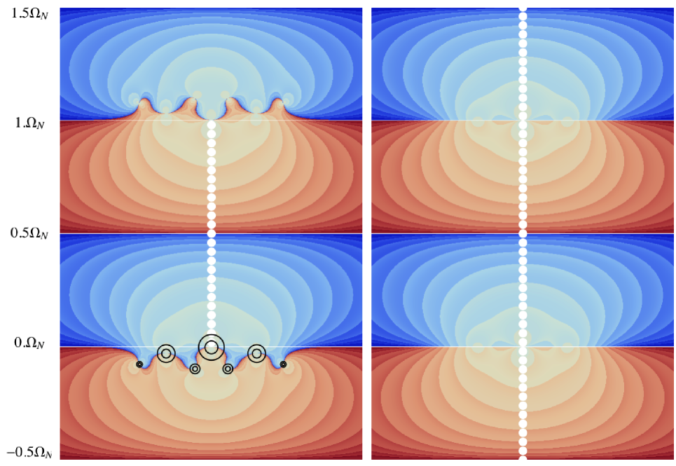
Figure 3: (Color online) Analytic structure of the Green’s function $G_{\epsilon_{k}=0}(z)$. In (a) the branch ($G^{R}$) which is analytic in $0<Im\,z<\Omega_{N}$. $Im(G)$ is plotted as in Fig. 2c. In (b) the corresponding periodic Green’s function with branch cuts at integer multiples of $i\Omega_{N}$. ($Imz$ in units of $\Omega_{N}=\frac{2\pi N}{\beta}$)

and using the same countour integral it can also shown be that $L(\omega)$ is properly normalized: $\int_{-\infty}^{\infty}\frac{d\omega}{2\pi}L(\omega)=1$. The function $G(z)$ is thus completely free from singularities in the strip $0<Imz<\Omega_{N}$ and has poles outside the strip at $\epsilon-i\gamma$ and $\epsilon+i\gamma+i\Omega_{N}$ and obeys $G(z)=G(z+2i\Omega_{N})$ as shown in Figure 3a. In the limit $\eta\rightarrow 0$ the function reduces to $G(z)=\frac{1}{z-(\epsilon-i\gamma)}$ which is the usual retarded Green’s function from a Lorentzian spectral weight. Evaluating $G(z)$ in the strip $-\Omega_{N}<Imz<0$ gives an expression which is analytic in that strip and which analogously corresponds to the advanced Green’s function. The full analytic Green’s function with periodically repeated branch cuts corresponds to gluing together the two branches as indicated in Figure 3b. In the limit $\eta\rightarrow 0$, $\Omega_{N}=\pi/\eta\rightarrow\infty$ thus reproducing the standard structure of the analytic Green’s function with a branch cut on the real axis.

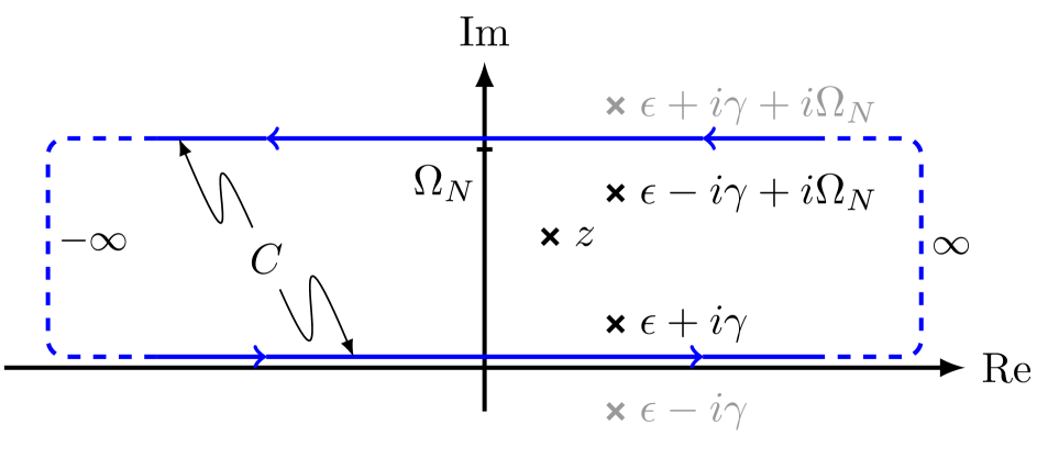
Figure 1: (Color online) Contour for the integration of Eq. 8

Let us now consider a spectral function defined by a set of such “periodized Lorentzians” $L_{\epsilon_{\nu},\gamma_{\nu}}(\omega)$. For $0<Im\,z<\Omega_{N}$ we find

$$G(z)=\frac{\eta}{2}\sum_{\nu}[a_{\nu}\coth\frac{\eta}{2}(z-\epsilon_{\nu}+i\gamma_{\nu})+$$ (9)

$$a^{*}_{\nu}\tanh\frac{\eta}{2}(z-\epsilon_{\nu}-i\gamma_{\nu})]\,,$$

where we have allowed for a complex prefactor $a_{\nu}$ that must satisfy $\frac{1}{2}\sum_{\nu}(a_{\nu}+a^{*}_{\nu})=1$ to conserve total spectral weight. Given a set of values of $G_{n}\equiv G_{k}(i\omega_{n})$ we would like to extract the values of $a_{\nu}$, $e_{\nu}$ and $\gamma_{\nu}$ that solves Eq. 9. The latter can be cast into the form of a rational function containing only simple poles (as opposed to periodically repeated) by means of the conformal mapping

$$z^{\prime}=\coth(\frac{\eta}{2}z-i\frac{\pi}{4})$$ (10)

which gives

$$G(z^{\prime})=\frac{\eta}{2}\sum_{\nu=1}^{n}\left(a_{\nu}\frac{1-p_{\nu}z^{\prime}}{z^{\prime}-p_{\nu}}+a^{*}_{\nu}\frac{1-p^{*}_{\nu}z^{\prime}}{z^{\prime}-p^{*}_{\nu}}\right)\,,$$ (11)

with $p_{\nu}=\coth(\frac{\eta}{2}(\epsilon_{\nu}-i\gamma_{\nu})-i\frac{\pi}{4})$. The transformation maps the strip $0\leq Imz<2\Omega_{N}$ to the entire complex plane. The strip $\Omega_{N}\leq Im\ z<2\Omega_{N}$ that contains the singularities is mapped to the interior of the unit circle and the strip $0<Im\,z<\Omega_{N}$ that is free from singularities is outside, as exemplified in Figure 2c and d. The points $z=\pm\infty$ on the real axis map to $z^{\prime}=\pm 1$ and the point $z=i\omega_{(N-1)/2}$ maps to $z^{\prime}=\infty$.

The function $G(z^{\prime})$ should obey a number of properties. Since Eq. 11 can be written as a rational function $G(z^{\prime})=const+P(z^{\prime})/Q(z^{\prime})$ where $P$ is an $M-1$ degree and $Q$ is an $M^{\prime}th$ degree polynomial of $z^{\prime}$ and $const=-\frac{\eta}{2}\sum(a_{\nu}p_{\nu}+a_{\nu}^{*}p_{\nu}^{*})$, we can identify $p_{\nu}$ with the roots of $Q$ and $\frac{\eta}{2}(1-p_{\nu}^{2})a_{\nu}$ as the residues of $P/Q$. Taking $N$ odd gives a precise boundary condition $G(z^{\prime}=\infty)=const=G_{(N-1)/2}$. We also require $G(z^{\prime}=1)=-G(z^{\prime}=-1)=\frac{\eta}{2}\sum_{\nu}(a_{\nu}+a^{*}_{\nu})=\eta$ to obtain the proper normalization. A crucial observation is that Eq. 3 preserves this condition independent of ${\bar{\Sigma}}$ and demonstrates that total spectral weight is preserved by the periodized Dyson equation. By straightforward calculation from Eq. 5 we also conclude that $G^{\prime}(z=1)=G^{\prime}(z=-1)=0$ which further constrains the analytic continuation. We thus find $P(z^{\prime})$ and $Q(z^{\prime})$ by fitting $G(z^{\prime})-const$ to $(M-1)/M$ Padé form, yielding $M=(N+3)/2$. In addition we have the symmetry $G(i\omega_{N-1-n})=G^{*}(i\omega_{n})$ resulting in $M/2$ independent poles. Thus $n=(N+3)/4$ in Eq. 11. Having identified the parameters $a_{\nu}$ and $p_{\nu}$ in the fit, the spectral function can be evaluated through $A(\omega)=-2ImG(\omega)$ using Eq 9. For every value of $N$ we can also obtain a properly normalized spectral weight using $A(\omega)=2\sum_{\nu}\frac{Rea_{\nu}\gamma_{\nu}-Ima_{\nu}(\omega-\epsilon_{\nu})}{(\omega-e_{\nu})^{2}+\gamma_{\nu}^{2}}$ resulting in Green’s function with the proper discontinuity $G_{k}(\tau=0^{-})-G_{k}(\tau=0^{+})=\int_{-\infty}^{\infty}\frac{d\omega}{2\pi}A(k,\omega)=1$.

We tested our method on the Dynamical mean field theory (DMFT) method using the IPT approximation with the half filled paramagnetic Hubbard model.George_Kotliar92 ; George_review ; Potthoff ; Hugo We found that the convergence was significantly enhanced by evaluating the dynamic part of the self energy as $\tanh\eta\Sigma(i\omega_{n})=\eta U^{2}{\cal F}\left(G^{3}_{0,imp}(\tau_{j})\right)$ where Eq. 1 has been used. This expression ensures that $Im\Sigma$ lies within the appropriate bounds and by expanding $\tanh$ in powers of $\Sigma$ it is equivalent to the standard expression to order $U^{2}$. The detailed implications of this procedure should be explored further.

Figure 2 shows the spectral function for varying bare energy $A(\epsilon_{k},\omega)$ at $\beta=25$ ($T=W/50$), in the metallic, $U=2$ (with $N=25$), and insulating, $U=4$ ($N=45$) phases using the standard semicircular bare density of statesHugo and 40 significant digits to compute the rational function. This gives 7 and 12 independent complex poles respectively. The location of poles are indicated in Fig. 2 for $\epsilon_{k}=0$. Since $\Sigma$ is $k$-independent we can extract it with a single Padé fit and use this to generate the spectral function for any $\epsilon_{k}$. We have found that the number of frequencies needed is roughly $N\gtrsim\beta$ for convergence of the IPT recursion algorithm and as further test we have used the method at low temperature $\beta\geq 500$ and a number of significant digits roughly also equal to $N$.

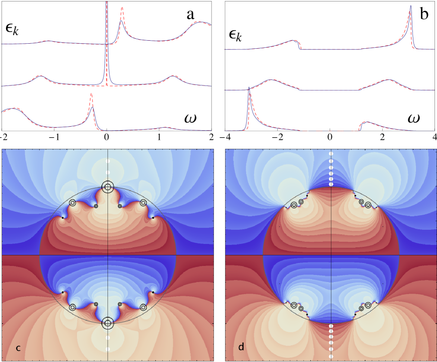
Figure 2: (Color online) Spectral functions $A(\epsilon_{k},\omega)$ at $\beta=25$ for metal $U=2$ (a) and insulator $U=4$ (b) for bare energies $\epsilon_{k}=-1,0,1$. (Dashed curves are $\beta=500$ and $\beta=200$ respectively.) The corresponding $Im(G_{\epsilon_{k}=0}(z^{\prime}))$ is shown in (c) and (d) including circles marking the location of poles. The poles are located inside the unit circle in accordance with Eq. 11. Empty dots represent a subset of the Matsubara values ($z^{\prime}(i\omega_{n})$). The color scale is light for large positive and negative values with dark colors near zero.

As a second test of the analytic continuation method, we considered a noninteracting single impurity Anderson model whose spectral function consists of a sharp resonance as well as a continuum. These features have been found to be difficult to reproduce in detail using ordinary Padé methods.schon We used Eq. 5 to compute $G_{imp}(i\omega_{n})$ from the exact $A_{imp}(w)$ using $N=61$, $\beta=25$, and 60 significant figures. Using this we find 16 independent complex poles that to the eye reproduces the exact spectral function. It has an integrated rms deviation over total weight (excluding the resonance) of $4\cdot 10^{-3}$. The resonance has a width of $10^{-8}$ and a normalization which is within $10^{-5}$ of the exact value. A major reason for our success is the high precision for the Padé fit rather than a large number of poles. Fitting a greater number of less accurate data points does not yield comparable accuracy. This motivates using our method to compute a Green’s function to extremely high precision in a relatively small dimensional space and to use the combination of conformal transformation and Padé fit to infer the analytic continuation to the real axis.

We have presented a method to work with discrete-time Matsubara Green’s functions. In spite of working in a finite dimensional space the method yields an analytic continuation that obeys the boundary condition at $\tau=0$, a problem that has plagued other previous discretization schemes. Within this small space, numerical calculations can be done to the extremely high accuracy that is necessary to numerically obtain a meaningful analytic continuations from imaginary to the real time axis. The method should have wide applicability to all problems requiring numerical evaluation of Matsubara Green’s function in condensed matter physics nuclear physics and quantum field theory.

References

(1) A.A. Abriksov, L.P. Gorkov, I.E. Dzyaloshinskii, Quantum field theoretical methods in many body physics., (2ed, Pergamon, 1965).
(2) J.W. Negele, and H. Orland, “Quantum Many-Particle Systems”, Addison-Wesley, 1988.
(3)H. J. Vidberg and J. W. Serene, J. Low Temp. Phys. 29 , 179 (1977).
(4) R.N. Silver,
J.E. Gubernatis,
D.S. Sivia,
and M. Jarrell, Phys. Rev. Lett. 65, 496 (1990).
(5) By numerically exact we mean a convergent solution
computable to any number of significant figures with a realistic amount of computer time. Calculations
were done using arbitrary precision arithmetic in Mathematica. We have had no
trouble performing calculations with several hundred significant digits in order to resolve
a large number of poles in the Greens function.
(6) It should be noted for any calculation for regularly spaced imaginary time coordinates,
be it quantum Monte Carlo or perturbative Greens function calculations, the natural expansion
is a Greens function of the form Eq. 1 that fits all the “Matsubara” data rather
than a direct fit of the continuum form .
(8) G. Baym,
Progress in nonequilibrium Green’s functions,
Proceedings of the conference, “Kadanoff-Baym Equations Progress and Perspectives for Many-body Physics”, Rostock Germany, 20-24 September, 1999.
(9) A. Georges, and G. Kotliar, Phys. Rev B 45, 6479 (1992).
(10) A. Georges, G. Kotliar, W. Krauth, M. Rozenberg, Rev. Mod. Phys. 68, 1996.
(11) M. Potthoff, Adv. in Solid State Physics, 45,, 135 (2006); Eur. Phys. Journal B, 36, 2003.
(12) H.U.R. Strand, A. Sabashvili, M. Granath, B. Hellsing, S. Östlund
Phys. Rev. B 83 , 205136 (2011).
(13) C Karrasch,R Hedden, R Peters, Th Pruschke,K Schonhammer and V Meden,
J. Phys.: Condens. Matter 20 345205 (2008); C. Karrasch, V. Meden, and K. Schönhammer,
Phys. Rev. B 82 , 125114 (2010).