Bias in low-multipole CMB reconstructions

Abstract

The large-angle, low multipole cosmic microwave background (CMB) provides a unique view of the largest angular scales in the Universe. Study of these scales is hampered by the facts that we have only one Universe to observe, only a few independent samples of the underlying statistical distribution of these modes, and an incomplete sky to observe due to the interposing Galaxy. Techniques for reconstructing a full sky from partial sky data are well known and have been applied to the large angular scales. In this work we critically study the reconstruction process and show that, in practise, the reconstruction is biased due to leakage of information from the region obscured by foregrounds to the region used for the reconstruction. We conclude that, despite being suboptimal in a technical sense, using the unobscured region without reconstructing is the most robust measure of the true CMB sky. We also show that for noise free data reconstructing using the usual optimal, unbiased estimator may be employed without smoothing thus avoiding the leakage problem. Unfortunately, directly applying this to real data with noise and residual, unmasked foregrounds yields highly biased reconstructions requiring further care to apply this method successfully to real-world CMB.

1 Introduction

Several prominent anomalies in the large-angle, low-$\ell$ cosmic microwave background (CMB) have been identified, starting with pioneering observations by the Cosmic Background Explorer (COBE) (Bennett et al., 1996), and confirmed and extended with the high precision observations from the Wilkinson Microwave Anisotropy Probe (WMAP) (Bennett et al., 2003). These anomalies include the unexpectedly low correlations at scales above 60 degrees (Bennett et al., 1996, 2003; Copi et al., 2010; Sarkar et al., 2011),the alignments of the largest multipoles with each other and the Solar System (de Oliveira-Costa et al., 2004; Schwarz et al., 2004; Land & Magueijo, 2005; Copi et al., 2006), a parity asymmetry at low multipoles (Kim & Naselsky, 2010a, b, d, c), and the spatial asymmetries in the distribution of power observed at smaller scales (Eriksen et al., 2004a, b; Hansen et al., 2009). Numerous attempts have been made to explain or explain away these anomalies (Slosar & Seljak, 2004; Hajian, 2007; Afshordi et al., 2009; Bennett et al., 2011) – none of them successful (see Copi et al., 2010, and references therein, for a review).

The most peculiar and robust CMB anomaly is arguably the lack of correlation on large angular scales first observed by COBE (Bennett et al., 1996) and confirmed and further quantified through the $S_{1/2}$ statistic by WMAP (Spergel et al., 2003). Subsequent study of the two point angular correlation function, $C(\theta)$, has found further oddities; the large angle correlation is mainly missing outside of the Galactic region, there being essentially no correlation on large angles. The large-angle correlation that is observed comes from the foreground removed Galactic region of the reconstructed full-sky map (Copi et al., 2009). From the internal linear combination (ILC) map, the full-sky map created from the individual frequency bands which provides our best picture of the full sky microwave background radiation, it is found that the lack of correlation is unlikely at the approximately $95$ per cent level. However, when solely the region outside the Galaxy of the individual frequency or ILC maps are analysed the lack of correlation is rare at the approximately $99.975$ percent level (Copi et al., 2009).

The study of the large-angle CMB presents special problems that must be treated carefully. Since there is only one Universe to observe and few independent modes at low-$\ell$, large sky coverage is needed, and even with this coverage, very little independent information about the ensemble is available. Further, given the observed low quadrupole power, $C_{2}^{\mathrm{o}bs}\sim 100$–$200\;\mathrm{(\mathrm{\mu K})^{2}}$, compared to the best fit $\Lambda$CDM model, $C_{2}^{\Lambda\mathrm{CDM}}\sim 1300\;\mathrm{(\mathrm{\mu K})^{2}}$, large-angle studies are particularly sensitive to assumptions and unintended biases.

One suggestive example of this is provided by the ILC map itself. If we use a pixel based estimator for the $C_{\ell}$ as implemented in SpICE (Chon et al., 2004) we can easily determine the quadrupole power inside and outside the WMAP provided analysis mask KQ75y7 to be

$$C_{2}^{\mathrm{inside}}\approx 610\;\mathrm{(\mathrm{\mu K})^{2}},\qquad C_{2}^{\mathrm{outside}}\approx 80\;\mathrm{(\mathrm{\mu K})^{2}}.$$ (1)

The KQ75y7 mask cuts out approximately $25$ percent of the sky. Taking the weighted average of these values produces the intriguing result

$$0.25C_{2}^{\mathrm{inside}}+0.75C_{2}^{\mathrm{outside}}\approx 200\;\mathrm{(\mathrm{\mu K})^{2}},$$ (2)

a value consistent with the WMAP reported $C_{2}$ (Larson et al., 2011). Again we stress this is a suggestive example, not a careful analysis; the pseudo-$C_{\ell}$ (PCL) estimator employed here is suboptimal, we have not include errors on the estimates, etc. It does, however, show the wide discrepancy between the Galactic region and the rest of the sky, a common theme for the ILC map. Further it shows how a large value mixed in from a small region of the sky significantly impacts the final result.

In a recent paper Efstathiou et al. (2010), the authors claimed that the low $S_{1/2}$ results are due to the use of a suboptimal estimator (the pixel based estimator) of $C(\theta)$ and proposed an alternative based on reconstructing the full sky. This proposal avoids addressing the question of why the partial sky contains essentially no correlations on large angular scales and instead focuses on a new question that centre on the issue of how the full sky is reconstructed. In this work we carefully study full-sky reconstruction algorithms and their effects on the low-$\ell$ CMB.

It is well known that contamination affects the reconstruction of the low multipoles (Bielewicz et al., 2004; Naselsky et al., 2008; Liu & Li, 2009; Aurich & Lustig, 2010). In particular Aurich & Lustig (2010) have found that smoothing of full sky map prior to analysis, as required by a reconstruction algorithm (see Efstathiou et al. (2010) and our discussion below) leaks information from from the region inside the mask to pixels outside the mask. They showed that the pixels outside the mask have errors that are a significant fraction of the mean CMB temperature. They further find that it is safest to calculate the two point angular correlation function on the cut-sky. Here we confirm and extend these results.

Alternative analyses such as that suggested in Efstathiou et al. (2010), must be performed with care. In this work we carefully study the full-sky reconstruction, based on the cut-sky data, in a Universe with low quadrupole power. In Sec. 2 we briefly present the formalism typically employed in CMB studies. Sec. 3 contains our results and we conclude in Sec. 4. Ultimately we find that if a full-sky map, such as the ILC, is a faithful representation of the true CMB sky, then a reconstruction algorithm can reproduce its properties. This is not surprising: if the full-sky map is already trusted, there is no need to perform a reconstruction and nothing is gained by doing so. However, if part of the full sky is not trusted or is known to be contaminated, then, by reconstructing without properly accounting for the assumptions implicit in the algorithm, the final results will be biased toward the full-sky values. Again this is not surprising, if information from the questioned region is allowed to leak into the rest of the map then it will affect the final results and nothing will be learned about the validity of the reconstruction.

In any reconstruction of unknown values from the properties of existing data assumptions must be made. Often these assumptions are not explicitly stated. For the work presented here we take the observed microwave sky outside of the Galactic region as defined through the KQ75y7 mask to be a fair sample of the CMB. This partial-sky region is known to have essentially no correlations on large angular scales; it is unlikely in the best fit $\Lambda$CDM model at the $99.975$ per cent level (Copi et al., 2009). Our study shows the bias introduced into full-sky reconstructions when an admixture of a region with larger angular correlations is included prior to reconstruction. We stress that results of the partial-sky analysis are not being questioned, instead a new question is being asked; how should the full sky be reconstructed when there is a wide disparity between the statistical properties of the region outside the Galaxy and that inside.

2 Reconstruction Formalism

Optimal, unbiased estimators for both the $C_{\ell}$ and $a_{\ell m}$ are well known and discussed extensively in the literature (see, for example, Tegmark, 1997; Efstathiou, 2004; de Oliveira-Costa & Tegmark, 2006; Efstathiou et al., 2010). Here we provide a brief overview of the maximum likelihood estimator (MLE) technique and introduce our notation. For details including discussions of invertability of the matrices, proofs of optimality, etc., see the references.

The microwave temperature fluctuations on the sky can be represented by the vector $\mn@boldsymbol{x}(\mn@boldsymbol{\hat{e}}_{j})$,

$$\mn@boldsymbol{x}=\textbf{{Y}}\mn@boldsymbol{a}+\mn@boldsymbol{n},$$ (3)

where Y is the matrix of the $Y_{\ell,m}(\mn@boldsymbol{\hat{e}}_{j})$, $j$ runs over all pixels on the sky, $\mn@boldsymbol{\hat{e}}_{j}$ is the radial unit vector in the direction of pixel $j$, $\mn@boldsymbol{a}$ is the vector of $a_{\ell m}$ coefficients, and $\mn@boldsymbol{n}$ is the noise in each pixel. For the work considered here we are only interested in the large-angle, low-$\ell$ behaviour so we assume that $\mn@boldsymbol{n}$ can be ignored and set $\mn@boldsymbol{n}=0$ in what follows. When working with the WMAP data at low resolution this is justified, for example the W band maps at $\textsc{Nside}=16$ have pixel noise $\sigma_{\mathrm{pix}}<3\;\mathrm{\mathrm{\mu K}}$. At higher resolution this is not as clearly justified. In this work we study reconstruction bias independent of pixel noise so we may ignore $\mn@boldsymbol{n}$ for our simulations. When setting $\mn@boldsymbol{n}=0$ are further assuming that the region we are analysing is free of foregrounds. This is a standard, though implicit, assumption when reconstructions are performed. The covariance matrix is then given by

$$\textbf{{C}}=\langle\mn@boldsymbol{x}{\mn@boldsymbol{x}}^{\mathsf{T}}\rangle=\textbf{{S}}.$$ (4)

Here the angle brackets, $\langle\cdot\rangle$ represent an ensemble average. This is the expectation value of the theoretical two point angular correlation function, not its measured value. As is customary, we call S the signal matrix despite the fact that it is not the two point angular correlation measured on the sky. We do not include a noise matrix, N, in our covariance since we are neglecting noise.

2.1 Reconstructing the $\mn@boldsymbol{a_{\ell m}}$

To reconstruct the $a_{\ell m}$ we define the signal matrix as the two point angular correlation function of the unreconstructed modes

$$\textbf{{C}}=\textbf{{S}}=\sum_{\ell=\ell_{\mathrm{recon}}+1}^{\ell_{\mathrm{max}}}C_{\ell}\textbf{{P}}^{\ell}.$$ (5)

Here $\textbf{{P}}^{\ell}$ is the matrix of the weighted Legendre polynomials,

$$\textbf{{P}}^{\ell}_{i,j}\equiv\frac{2\ell+1}{4\pi}P_{\ell}(\mn@boldsymbol{\hat{e}}_{i}\cdot\mn@boldsymbol{\hat{e}}_{j}),$$ (6)

and we assume all modes with $2\leq\ell\leq\ell_{\mathrm{recon}}$ are to be reconstructed. Here $\ell_{\mathrm{max}}$ is the maximum multipole considered. We have chosen $\ell_{\mathrm{max}}=4\textsc{Nside}+2$ for this work. The optimal, unbiased estimator is then given by (de Oliveira-Costa & Tegmark, 2006)

$$\hat{\mn@boldsymbol{a}}=\textbf{{W}}\mn@boldsymbol{x},\qquad\textbf{{W}}\equiv[{\textbf{{Y}}}^{\mathsf{T}}\textbf{{C}}^{-1}\textbf{{Y}}]^{-1}{\textbf{{Y}}}^{\mathsf{T}}\textbf{{C}}^{-1}.$$ (7)

Note that here and throughout we work in the real spherical harmonic basis, so Y is a real matrix. The covariance matrix of our estimator is

$$\Sigma\equiv\langle\hat{\mn@boldsymbol{a}}{\hat{\mn@boldsymbol{a}}}^{\mathsf{T}}\rangle-\langle\hat{\mn@boldsymbol{a}}\rangle{\langle\hat{\mn@boldsymbol{a}}\rangle}^{\mathsf{T}}=[{\textbf{{Y}}}^{\mathsf{T}}\textbf{{C}}^{-1}\textbf{{Y}}]^{-1}.$$ (8)

The signal matrix, C, need not include all pairs of pixels on the sky. When it does, a reconstruction will produce precisely the spherical harmonic decomposition. Conversely, when a sky is masked, we only include the unmasked pixels in C. The process of ‘masking’ is thus performed by removing the masked pixels from the signal matrix, and this process is equivalent to assigning infinite noise to the masked pixels.

2.2 Reconstructing the $\mn@boldsymbol{C_{\ell}}$

To reconstruct the $C_{\ell}$ we define the signal matrix as the two point angular correlation of all the modes;

$$\textbf{{C}}=\textbf{{S}}=\sum_{\ell=2}^{\ell_{\mathrm{max}}}C_{\ell}\textbf{{P}}^{\ell}.$$ (9)

Notice that this differs from our previous definition (5). The optimal, unbiased estimator for the $C_{\ell}$ is then constructed from an unnormalized estimator, $\mn@boldsymbol{y}_{\ell}$. Let

$$\mn@boldsymbol{y}_{\ell}\equiv{\mn@boldsymbol{x}}^{\mathsf{T}}\textbf{{E}}^{\ell}\mn@boldsymbol{x},\qquad\textbf{{E}}^{\ell}\equiv\frac{1}{2}\textbf{{C}}^{-1}\textbf{{P}}^{\ell}\textbf{{C}}^{-1}.$$ (10)

The correlation matrix of this estimator is the Fisher matrix,

$$\textbf{{F}}_{\ell,\ell^{\prime}}=\langle\mn@boldsymbol{y}_{\ell}{\mn@boldsymbol{y}_{\ell^{\prime}}}^{\mathsf{T}}\rangle-\langle\mn@boldsymbol{y}_{\ell}\rangle{\langle\mn@boldsymbol{y}_{\ell^{\prime}}\rangle}^{\mathsf{T}}=\frac{1}{2}\mathop{\mathrm{Tr}}\nolimits\bigl{[}\textbf{{C}}^{-1}\textbf{{P}}^{\ell}\textbf{{C}}^{-1}\textbf{{P}}^{\ell^{\prime}}\bigr{]}.$$ (11)

Finally, this gives the optimal, unbiased estimator of the $C_{\ell}$,

$$\hat{C}_{\ell}=\sum_{\ell^{\prime}}\textbf{{F}}^{-1}_{\ell,\ell^{\prime}}\mn@boldsymbol{y}_{\ell^{\prime}}.$$ (12)

Though the full Fisher matrix can be calculated, it turns out to be nearly diagonal for reasonably small masks such as the WMAP KQ75y7 mask. In this case the approximations

$$\textbf{{F}}_{\ell,\ell^{\prime}}\approx\frac{2\ell+1}{2\hat{C}_{\ell}^{2}}\delta_{\ell,\ell^{\prime}},\qquad\textbf{{F}}_{\ell,\ell^{\prime}}^{-1}\approx\frac{2\hat{C}_{\ell}^{2}}{2\ell+1}\delta_{\ell,\ell^{\prime}}$$ (13)

may be employed. We have confirmed the validity of this approximation and have employed it when applicable in our subsequent analyses.

2.3 Relating the Estimators

The optimal, unbiased estimators for $a_{\ell m}$ and $C_{\ell}$ are related to each other. If we define the weighted harmonic coefficients by

$$\mn@boldsymbol{\beta}\equiv\Sigma^{-1}\hat{\mn@boldsymbol{a}},$$ (14)

then

$$\mn@boldsymbol{y}_{\ell}=\frac{1}{2}\sum_{m}|\beta_{\ell m}|^{2}$$ (15)

is identical to (10) from which we may calculate $\hat{C}_{\ell}$ (de Oliveira-Costa & Tegmark, 2006; Efstathiou et al., 2010).

In our discussion we have been careful to note that C is defined differently when used as an estimator for the $a_{\ell m}$ versus the $C_{\ell}$. In practise when the signal-to-noise is large the estimator for the $a_{\ell m}$ is not sensitive to the precise values and range of the $C_{\ell}$ employed. However, to find $\hat{C}_{\ell}$ from $\hat{\mn@boldsymbol{a}}$ through the weighted harmonic coefficients (14), the full signal matrix (9) must be used when calculating the covariance matrix (8) and Fisher matrix (11).

The above discussion shows that Eq. (12) is the optimal, unbiased estimator for the $C_{\ell}$. Even so, given $\hat{\mn@boldsymbol{a}}$ from (7) it is tempting to define a naive estimator for the $C_{\ell}$ via

$$C_{\ell}^{e}\equiv\frac{1}{2\ell+1}\sum_{m}|\hat{\mn@boldsymbol{a}}_{\ell m}|^{2}$$ (16)

and use this to reconstruct $C(\theta)$ (see fig. 5 of Efstathiou et al., 2010). In general this is a poor definition for the estimator as clearly an optimal, unbiased estimator for some quantity does not provide an optimal, unbiased estimator for the square of that quantity. Its use leads to a biased estimator for the $C_{\ell}$ and a biased reconstruction of $C(\theta)$. We will explore both this estimator and the optimal, unbiased one below.

2.4 Two Point Angular Correlation Function

The two point angular correlation function is defined as a sky average, that is by a sum over all pixels on the sky separated by the angle $\cos\theta_{i,j}=\mn@boldsymbol{\hat{e}}_{i}\cdot\mn@boldsymbol{\hat{e}}_{j}$,

$$C(\theta_{i,j})\equiv\sum_{i,j}\mn@boldsymbol{x}_{i}\mn@boldsymbol{x}_{j}.$$ (17)

Ideally the two point angular correlation function would also contain an ensemble average over realisations of the underlying model. Since we only have one Universe, this ensemble average cannot be calculated. However, for a statistically isotropic Universe the sky average and ensemble average are equivalent. This definition has the additional benefit that it can be calculated on a fraction of the sky.

Alternatively the two point angular correlation function may be expanded in a Legendre series,

$$C(\theta_{i,j})=\sum_{\ell}\frac{2\ell+1}{4\pi}C_{\ell}P_{\ell}(\cos\theta_{i,j}).$$ (18)

Note that for partial sky coverage or lack of statistical isotropy the $C_{\ell}$ in this this expression are not the same as the $\hat{C}_{\ell}$ obtained from the $a_{\ell m}$; see Copi et al. (2007) for a discussion. This subtlety will not be important for the following work.

2.5 $\mn@boldsymbol{S_{1/2}}$ Statistic

To quantify the lack of large-angle correlations the $S_{1/2}$ statistic has been defined by Spergel et al. (2003) to be

$$S_{1/2}\equiv\int_{-1/2}^{1}\left[C(\theta)\right]^{2}\mathrm{d}(\cos\theta).$$ (19)

Expanding $C(\theta)$ in terms of the $C_{\ell}$ as above (18) we find

$$S_{1/2}=\sum_{\ell,\ell^{\prime}}C_{\ell}\mathcal{I}_{\ell,\ell^{\prime}}C_{\ell^{\prime}},$$ (20)

where

$$\mathcal{I}_{\ell,\ell^{\prime}}\equiv\frac{(2\ell+1)(2\ell^{\prime}+1)}{(4\pi)^{2}}\int_{-1/2}^{1}P_{\ell}(\cos\theta)P_{\ell^{\prime}}(\cos\theta)\mathrm{d}(\cos\theta)$$ (21)

is a known matrix (see Copi et al. 2010) that can be evaluated.

The estimator generally employed for $S_{1/2}$ is

$$\hat{S}_{1/2}=\sum_{\ell,\ell^{\prime}}\hat{C}_{\ell}\mathcal{I}_{\ell,\ell^{\prime}}\hat{C}_{\ell^{\prime}}.$$ (22)

Even with $\hat{C}_{\ell}$ itself an optimal, unbiased estimator of $C_{\ell}$, this does not produce an optimal, unbiased estimator for $S_{1/2}$ (Pontzen & Peiris, 2010). For the unbiased estimator (12) we have

$$\langle\hat{C}_{\ell}\hat{C}_{\ell^{\prime}}\rangle = \sum_{\tilde{\ell},\tilde{\ell}^{\prime}}\textbf{{F}}_{\ell,\tilde{\ell}}^{-1}\textbf{{F}}_{\tilde{\ell}^{\prime},\ell^{\prime}}^{-1}\langle y_{\tilde{\ell}}{y_{\tilde{\ell}^{\prime}}}^{\mathsf{T}}\rangle$$ (23)

$$= \sum_{\tilde{\ell},\tilde{\ell}^{\prime}}\textbf{{F}}_{\ell,\tilde{\ell}}^{-1}\textbf{{F}}_{\tilde{\ell}^{\prime},\ell^{\prime}}^{-1}\left(\langle y_{\tilde{\ell}}\rangle{\langle y_{\tilde{\ell}^{\prime}}\rangle}^{\mathsf{T}}+\textbf{{F}}_{\tilde{\ell},\tilde{\ell}^{\prime}}\right)$$

$$= \sum_{\tilde{\ell}}\left(\sum_{\tilde{\ell}^{\prime}}\langle\textbf{{F}}_{\ell,\tilde{\ell}}^{-1}y_{\tilde{\ell}}\rangle{\langle\textbf{{F}}_{\ell^{\prime},\tilde{\ell}^{\prime}}^{-1}y_{\tilde{\ell}^{\prime}}\rangle}^{\mathsf{T}}+\textbf{{F}}_{\ell,\tilde{\ell}}^{-1}\delta_{\ell^{\prime},\tilde{\ell}}\right)$$

$$\approx C_{\ell}C_{\ell^{\prime}}+\frac{2}{2\ell+1}C_{\ell}^{2}\delta_{\ell,\ell^{\prime}}.$$

In the second line we have used the definition of the Fisher matrix (11), the third line is an algebraic simplification, and in the final line we have again used (12), the fact that $\hat{C}_{\ell}$ is unbiased, and the approximation from (13). With this it now straightforward to see that

$$\langle\hat{S}_{1/2}\rangle = \sum_{\ell,\ell^{\prime}}\langle\hat{C}_{\ell}\hat{C}_{\ell^{\prime}}\rangle\mathcal{I}_{\ell,\ell}=S_{1/2}+\sum_{\ell}\frac{2C_{\ell}^{2}}{2\ell+1}\mathcal{I}_{\ell,\ell}$$ (24)

$$\neq S_{1/2}.$$

It is thus clear that (22) is a biased estimator and, in fact, is biased toward larger values of $S_{1/2}$.

As noted by Pontzen & Peiris (2010) this is of ‘pedagogical interest’ but does not affect the studies of low $S_{1/2}$. The Monte Carlo simulations employed (see Copi et al., 2009, for example) account for this bias. It does suggest that an alternative measure of the lack of large-angle correlations is desirable.

2.6 Assumptions

Efstathiou et al. (2010) claim that the full-sky, large-angle CMB can be reconstructed solely from the harmonic structure of the CMB outside the masked, Galactic region, and independent of the contents of the masked portion of the sky. We will demonstrate in what follows that this claim does not hold up to closer scrutiny.

It is clear that without assumptions regarding the harmonic structure inside the masked region nothing can be said about it. In principle the low-$\ell$ harmonic structure inside the masked region could be anything, ranging from no power, to large power, to wild oscillations, making the full-sky reconstruction impossible.

Assuming a cosmological origin for the observed microwave signal outside the masked region, it seems reasonable to assume it will be consistent with the signal inside the masked region. With that assumption, the harmonic structure outside the masked region can be extended into the masked region. For actual, full-sky maps there is a further assumption: the region inside the mask is well enough determined and statistically close enough to the region outside the mask that it does not bias the reconstruction. This latter assumption turns out to not be true as we demonstrate below.

Note also that if the region inside the mask is trusted, then there is no need to perform either masking or the reconstruction at all, the full-sky map can be analysed directly. Therefore, validity of the stringent assumptions required for the reconstruction obviates the very need for the reconstruction.

When the reconstruction formalism described above is applied to actual data, further assumptions are implicit. In our development we have assumed that the temperature fluctuations contain pure CMB signal. In practise, besides pixel noise (which we have not included as described above) the data may contain unknown foregrounds. To avoid contamination by foregrounds it is common to analyse a foreground-cleaned map, such as the ILC map, and to mask the most contaminated regions of the sky. In following this approach, care must be taken not to reintroduce contamination in the data prior to reconstruction. As we will show below, the standard process of preparing data for reconstruction, in particular smoothing the full-sky map, violates this requirement.

3 Results

To explore how data handling prior to reconstruction affects the results, we have performed a series of Monte Carlo simulations of $\Lambda$CDM based on reconstruction procedures suggested in the literature. We have employed the simplest best-fitting $\Lambda$CDM model from WMAP based solely on the WMAP data. This is model “lcdm+sz+lens” with “wmap7” data from the lambda site. Our results are insensitive to the exact details of the model since we are performing a theoretical study examine relative differences between reconstructions and not performing parameter estimation. Our simulations are performed at $\textsc{Nside}=128$ unless otherwise noted and we will focus on the reconstruction of $a_{2m}$ and $C_{2}$. Further, our simulations only consider $\ell_{\mathrm{recon}}=10$, reconstruct from the pixels outside the KQ75y7 mask provided by WMAP and degraded to the appropriate resolution, and use the data from the WMAP seven year release.

A collection of realisations of the full sky are created as follows:

1. Generate a random sky at $\textsc{Nside}=512$ from the best-fitting $\Lambda$CDM model.

2. Extract the $a_{2m}$ and calculate the power in the quadrupole, denote this value by $C_{2}$.

3. Rescale the $a_{2m}$ so that the $C_{2}$ in the map has a fixed value, for example, rescale so that $C_{2}=100\;\mathrm{(\mathrm{\mu K})^{2}}$ by replacing the $a_{2m}$ with $a_{2m}\rightarrow a_{2m}\sqrt{100\;\mathrm{(\mathrm{\mu K})^{2}}/C_{2}}$. Notice that this does not change the phase structure of the $a_{2m}$.

4. Smooth the map with a $10\degr$ Gaussian beam, if desired.

5. Degrade the map to the desired resolution ($\textsc{Nside}=128$ or $\textsc{Nside}=16$).

6. Repeat the rescaling of the $a_{2m}$ for each value of $C_{2}$ that we wish to consider. In our simulations we consider $C_{2}=10\mbox{--}10^{4}\;\mathrm{(\mathrm{\mu K})^{2}}$. This ensures that the same map realisation is used with only the quadrupole power changed.

This procedure constitutes a single realisation. The results in this work are based on at least $20,000$ realisations.

Degrading masks requires an extra processing step. Pixels near mask boundaries turn from the usual $1$ or $0$ to denote inclusion or exclusion from the analysis, respectively, to fractional values. We redefine our degraded masks by setting all pixels with a value greater than $0.7$ to $1$ and all others to $0$. For the KQ75y7 mask this process leaves about $70$ per cent of the pixels for analysis. To be precise, at $\textsc{Nside}=128$ this leaves $136,828$ unmasked pixels and at $\textsc{Nside}=16$ there are $2,157$ pixels left.

A map with a modest angular resolution contains all the low-$\ell$ CMB information, so it may seem surprising that we employ $\textsc{Nside}=128$ in our studies. Instead it is common in low-$\ell$ studies to employ a map at $\textsc{Nside}=16$, corresponding to pixels of approximately $3\degr$ in size (see Efstathiou et al., 2010, for a recent example of this). The effects of the choice of resolution, the need for smoothing a map prior to analysis, and the leaking of information this causes will now be explored.

3.1 Choice of Map Resolution

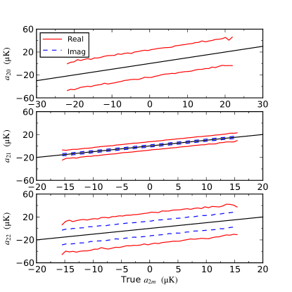
Figure 1: The $95$ and $5$ percentile lines for the $a_{2m}$ reconstructed from the pixels outside the KQ75y7 mask at $\textsc{Nside}=128$ (and thus $\ell_{\mathrm{max}}=514$) of $\Lambda$CDM realisations with $C_{2}=100\;\mathrm{(\mathrm{\mu K})^{2}}$, as discussed in the text. The red, solid lines are for the real part of the $a_{2m}$ and the blue, dashed lines are for the imaginary part. The black, solid line shows the expected result for a perfect reconstruction. We see that the reconstruction is unbiased, that is, it tracks the true value.

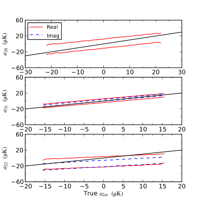
Figure 2: The same as Fig. 1 now reconstructed from the pixels outside the KQ75y7 mask at $\textsc{Nside}=16$ (and thus $\ell_{\mathrm{max}}=66$). Here we see that the reconstruction is biased.

The study of large-angle, low-$\ell$ properties of the CMB appears naively not to require high resolution maps. Maps degraded to the resolution corresponding to $\textsc{Nside}=16$ are commonly employed (de Oliveira-Costa & Tegmark, 2006; Efstathiou et al., 2010). When a map is degraded by averaging over pixels, high frequency noise is introduced as may be seen in Figs. 1 and 2. These figures show the reconstructed $a_{2m}$ using the optimal, unbiased estimator from Eq. (7) for realisations with $C_{2}=100\;\;\mathrm{(\mathrm{\mu K})^{2}}$. The solid, red lines (dashed, blue lines) show the $5$ and $95$ percentile lines from our realisations for the reconstructed real (imaginary) parts of each $a_{2m}$, using maps degraded to $\textsc{Nside}=128$ (Fig. 1) and $\textsc{Nside}=16$ (Fig. 2) and pixels outside the KQ75y7 mask. As expected from an unbiased estimator the reconstructed values track the true values (Fig. 1). Further we see that the $a_{21}$ are best determined and the $a_{20}$ and $a_{22}$ have larger variances due to the mask which produces greater admixture of ambiguous modes for these cases. However, for $\textsc{Nside}=16$ (Fig. 2) we see that the reconstruction does not track the true values and is instead biased. This bias is due to the averaging done to degrade the maps and becomes more significant the more the map is degraded. From this we conclude that the coupling of the small-scale modes to the large-scale modes caused by using maps with resolution that is too coarse can be at least partly responsible for reconstruction bias.

3.2 Smoothing the Map

Figure 3: The same as Fig. 1 now reconstructed from maps smoothed with a $10\degr$ Gaussian beam applied to the full sky map. As in Fig. 1, the reconstruction is unbiased.

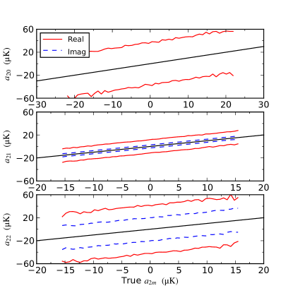
Figure 4: The same as Fig. 3 now reconstructed from maps with $\textsc{Nside}=16$. The reconstruction is now also unbiased.

In practise raw degraded maps are not used for the reasons shown in the previous section, instead the maps are smoothed with a Gaussian beam with FWHM of at least the size of the pixels and then degraded. In this work we employ a smoothing scale of $10\degr$, consistent with Efstathiou et al. (2010). Smoothing the maps studied in the previous section prior to reconstructing the $a_{\ell m}$ produces the results shown in Figs. 3 and 4. With smoothing we see that the $a_{\ell m}$ estimator is unbiased for both resolutions, $\textsc{Nside}=128$ and $\textsc{Nside}=16$. Smoothing is thus an essential step when working with low resolution maps.

In Figs. 3 and 4 we also see that the variance in the reconstructed values is resolution dependent with the smaller variance provided by the higher resolution maps. Again this is not surprising, and can be understood as follows. Our covariance matrix in Eq. (8) does not include a noise term yet we have introduced noise by degrading. Smoothing does a good job at reducing the noise to a level where the reconstruction is unbiased, however, there is still residual noise that affects the covariance of the estimator. The higher the resolution the smaller this noise. The best results are obtained by working at the highest resolution that is feasible. For this reason we work at $\textsc{Nside}=128$ in our simulations. See Appendix A for technical details.

3.3 Reconstructing the $\mn@boldsymbol{a_{\ell m}}$

We have now seen that the estimator in Eq. (7) is an optimal, unbiased estimator for the $a_{\ell m}$ when we work at high resolution and/or smooth the maps prior to reconstruction (Figs. 1, 3, 4). Although this has only been shown for $C_{2}=100\;\mathrm{(\mathrm{\mu K})^{2}}$ we have verified that this is true independent of the quadrupole power.

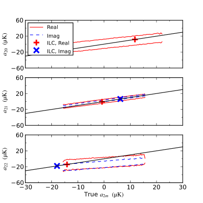
Figure 5: The same as Fig. 3 now with the masked region filled in with the ILC map prior to smoothing and rescaling. We clearly see the reconstructed $a_{2m}$ are not unbiased. The bias in reconstructing $a_{20}$ and $a_{22}$ is particularly apparent. This is due to the leakage of information from inside the masked region.

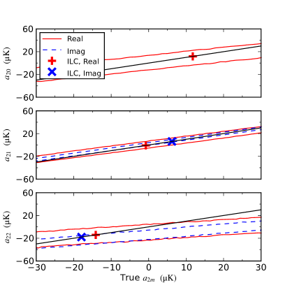
Figure 6: The same as Fig. 5 now with $C_{2}=1000\;\mathrm{(\mathrm{\mu K})^{2}}$.

As noted above, the fact that we are smoothing the maps prior to masking imposes assumptions on the maps. For the realisations discussed above the assumptions are met; the region inside the mask is, statistically, identical to the region outside. However, for real data the Galaxy is a bright foreground that must be removed. The WMAP ILC procedure attempts to do this and produce a full-sky CMB map. Even so, masking is often performed to avoid relying on the information inside this region since it may still be contaminated by Galactic foregrounds.

Unfortunately, when the map is smoothed information leaks out of the masked region and biases the reconstruction as shown in Figs. 5 and 6. For this analysis, for each synthetic map we filled the masked region with the corresponding portion (i.e. the masked region) taken from the ILC map. We then smoothed and degraded the resulting synthetic map. In these two figures we show the true and reconstructed values of the coefficients $a_{2m}$; we also show the ILC map’s $a_{2m}$ for reference. We clearly see the bias in the reconstructed $a_{2m}$ and its correlation with the ILC values. If $a_{2m}^{\mathrm{rec}}<a_{2m}^{\mathrm{ILC}}$, then $a_{2m}^{\mathrm{rec}}$ is biased upwards, and vice versa. For example, the ILC $a_{22}$ values are large and negative which leads to the reconstruction being skewed to agree better at large, negative values than at large positive values. This trend continues for the other $a_{2m}$ and clearly shows that the smoothing has mixed information from the masked region.

We can also recognise other details in the quality of the reconstruction that are specifically due to the orientation of the KQ75y7 mask in Galactic coordinates. For example, we see that the variance in the reconstructed real part of $a_{22}$ is larger than that for the imaginary part of $a_{22}$; the reason is that the real part of $Y_{22}$ has an extremum in the centre of the Milky Way where the mask ‘bulges’ while the imaginary part has a node at this location. Therefore, more information relevant to the real part of $a_{22}$ is missing than for the imaginary part, and the former has a larger reconstruction error. Moreover, it is also the case that the $Y_{20}$ and $Y_{22}$ have extrema in the Galactic plane whereas $Y_{21}$ has nodes. Due to this the variances of $a_{20}$ and $a_{22}$ are expected to be larger than that of $a_{21}$, as our reconstruction plots show.

Notice also that the reconstruction bias we find is not an artifact of the sharp transition introduced in the process of filling the masked regions of simulated maps with the ILC contents. The smoothing procedure, for one, completely removes the sharp feature in the map. Moreover, we have explicitly checked that the reconstructed $a_{\ell m}$ are not biased when the cut is filled with contents of another statistically isotropic map. Therefore, the reconstruction bias seen in our plots is real, and is caused to the specific structure of the ILC map behind the Galactic plane which ‘leaks’ into the unmasked region.

The question, then, is how to fill the masked region before smoothing. In principle anything could be used to fill the Galactic region, but then the information about this fill would leak outside the mask due to the smoothing. If the map were masked prior to smoothing then ‘zero’ would be leaked and bias the reconstruction. Alternatively, if the Galactic region were filled with Gaussian noise with root-mean-squared value consistent with the region outside the Galaxy then the estimator would be unbiased similar to the results in Fig. 1, but this would rely on the assumption that the true CMB inside the mask has precisely the same statistical properties as the CMB in the region outside. Filling with the ILC values would make sense if we could be completely confident that the ILC reconstruction of the region inside the mask is accurate. However, in the ILC the region inside the Galactic mask has different statistical properties than the region outside, particularly for the large-angle behaviour. This alone raises concerns that the ILC reconstruction is not entirely accurate. Further, if we knew how to properly treat the region inside the mask, either by accepting the ILC values or filling it with appropriate statistical values, there would be no need for a reconstruction as we would have a full sky map to analyse!

The challenge is that there is no, or at least no unique, compelling choice of how to fill the masked region before smoothing. In the face of this, the approach we take below is to study how the admixture of the large-angle behaviour of the Galactic region from the ILC map affects the reconstruction of the low-$\ell$ CMB, particularly when the region outside the Galaxy has low quadrupole power and lack of large-angle correlations. We show how this particular choice biases the reconstruction.

3.4 Reconstructing the $\mn@boldsymbol{C_{\ell}}$

Since we are interested in reconstructing $C(\theta)$ we next need to reconstruct the $C_{\ell}$. From the $a_{\ell m}$ we first proceed using the naive estimator (16), denoted $C_{\ell}^{e}$ (as used to generate fig. 5 of Efstathiou et al. 2010).

Figure 7: The $95$, $50$, and $5$ percentile lines of the reconstructed $C_{2}$ (top to bottom, respectively) from our realisations. The maps have not been smoothed prior to reconstruction. The pixel based (blue, solid line) comes from SpICE; where as, the reconstructed (red, dashed line) is the estimator $C_{\ell}^{e}$. We see that this estimator is clearly biased toward larger reconstructed values for small, true $C_{2}$, such as the values extracted from WMAP using either the PCL or MLE procedures. For a value of $C_{2}$ near the $\Lambda$CDM value the reconstruction method is a good estimator. The pixel based method produces values of $C_{2}$ with a median much closer to the true values, though with larger error bars.

The results for this estimator are shown in Fig. 7. For these realisations the maps were not smoothed. The reconstruction is shown as the dashed, red lines representing the $5$, $50$, and $95$ percentile values as a function of the true $C_{2}$ used to generate the maps. The solid, blue lines are the equivalent values from the reconstruction based on the pixel estimator from SpICE. Again the solid, black line is the reconstructed=true relation plotted to guide the eye. At large $C_{2}$ we see the desired behaviour: the reconstructed values from both estimators are centred around the true value, and $C_{2}^{e}$ does have a smaller variance, as an optimal estimator should (however, this does not mean it is optimal). At low $C_{2}$, in particular near the WMAP PCL and MLE values, the pixel based estimator is still centred around the true value, though with large variance; however, the $C_{2}^{e}$ is now biased toward larger values.

Figure 8: The same as Fig. 7 now with the realisations smoothed to $10\degr$ prior to reconstruction. It appears that the estimator (16) does a better job of reproducing $C_{2}$ for a $\Lambda$CDM model, though, see Fig. 9.

The results in Fig. 7 were for unsmoothed maps. The usual approach is to smooth the maps which suppresses power on small scales (high-$\ell$). Fig. 8 shows the results when the maps are smoothed prior to reconstruction; they are encouraging. Both estimators now track the true values much more closely. Even the median of $C_{2}^{e}$ remains close to the true value for values near the WMAP PCL value. This shows that with smoothing the correlations are reduced due to the lack of high frequency noise. It suggests that smoothing the map, reconstructing the $a_{\ell m}$, and employing $C_{\ell}^{e}$ as our estimator is sufficient and nearly optimal.

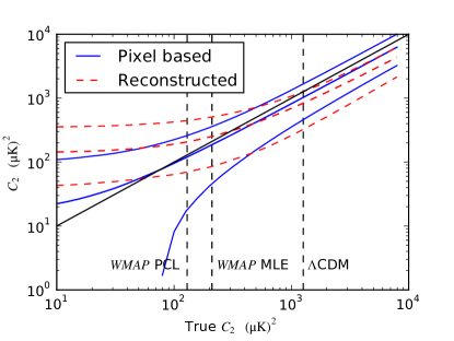
Figure 9: The same as Fig. 8 now with the region inside the masked replaced by the ILC prior to smoothing to $10\degr$ and reconstructing. Clearly the ILC information from inside the masked region has leaked out biasing the reconstruction. Not surprisingly the reconstruction now is only accurate near the WMAP MLE value; the value consistent with this region of the ILC. At lower $C_{2}$ values the reconstruction plateaus to this value as it is the main contribution to quadrupole power. At higher values of $C_{2}$ the quadrupole power is suppressed by the leakage.

Unfortunately this is not the case. As noted above, smoothing makes assumptions about the validity of the region inside the mask. We saw that even for the $a_{\ell m}$ this leads to a bias (see Fig. 5). When the corresponding ILC portion is placed into the masked region prior to smoothing the $C_{2}^{e}$ is also biased as shown in Fig. 9. We see that the masked region drives $C_{2}^{e}$ to be near the value inside the mask (approximately the WMAP MLE value). The $C_{2}^{e}$ results are biased upward for very small $C_{2}$ and downward for large $C_{2}$. Thus, even though smoothing helps in removing the correlation bias in the $C_{\ell}^{e}$ estimator it introduces its own bias. How the masked region is filled determines how the distribution of $C_{2}^{e}-C_{2}^{\mathrm{true}}$ will be skewed. Roughly speaking the values inside the mask will be favoured, raising the reconstructed values that are lower than the masked region values, and lowering values that are higher than those from the masked region.

We have seen that the naive estimator, $C_{\ell}^{e}$, provides an unbiased estimate of $C_{2}$ when the true value is near the expected, $\Lambda$CDM value. However, when the true value is low this estimator tends to overestimate $C_{2}$. Further, when smoothing is applied the reconstruction skews the values towards those consistent with the region inside the mask. This is to be expected. In fact, if the region inside the mask were believed then there would be no need to reconstruct at all, a full-sky map would already exist and it could be used for analysis without this extra effort.

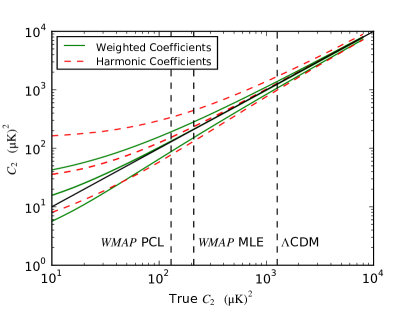
Figure 10: Similar to Fig. 8 now comparing $C_{2}^{e}$, the harmonic coefficient estimator (16) again as the dashed, red lines to $\hat{C}_{2}$, the weighted harmonic coefficient estimator (12) as the green, solid lines. We see that the weighted harmonic coefficient estimator is unbiased over the full true $C_{2}$ range.

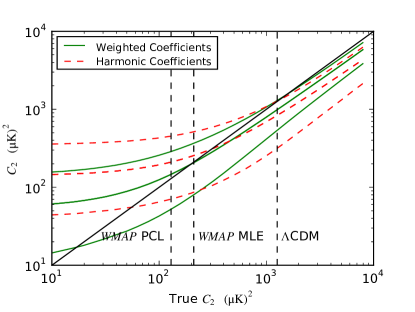
Figure 11: The same as Fig. 10 now for the Galactic region filled with the ILC values. We see that both estimators are now biased to agree best near the WMAP MLE value as we saw in Fig. 9.

3.5 Optimal, Unbiased $\mn@boldsymbol{C_{\ell}}$ Estimator

The general behaviour found for the naive estimator, $C_{\ell}^{e}$, carry over to the optimal, unbiased estimator, $\hat{C}_{\ell}$, based on the weighted harmonic coefficients (12), as we now see. Calculating $\hat{C}_{\ell}$ for the realisations considered above we find the results in Fig. 10 for Gaussian smoothed maps. This figure should be compared to Fig. 8. We see that $\hat{C}_{2}$ is nearly unbiased over the full range of true $C_{2}$ as expected.

The effect of smoothing when the ILC is inserted into the masked region is shown in Fig. 11. Again we see the bias introduced by smoothing when the two regions do not contain the same structure. These results are qualitatively similar to those found in Fig. 9 and the same discussion applies.

Table 1: $S_{1/2}$ values for the ILC map calculated for $2\leq\ell\leq 10$. The map is unprocessed, Gaussian smoothed with a $10\degr$ beam, or had the Galactic region filled with a Gaussian random, statistically isotropic sky realisation with the same power spectrum as the region outside this region prior to smoothing. The values are calculated for the full sky and for the KQ75y7 masked sky at $\textsc{Nside}=128$ using a pixel based estimator or the optimal, unbiased $C_{\ell}$ estimator (12) from maps at $\textsc{Nside}=128$ and $\textsc{Nside}=16$. The last row refers to the map whose mask area has been filled with Gaussian random field whose power is consistent with power measured outside the mask.

	$S_{1/2}\;(\mu\mathbf{K})^{4}$
ILC Map	Full Sky	Cut Sky	Reconstructed Sky
Processing		Pixel-	$\mathbf{N_{side}}$	$\mathbf{N_{side}}$
		based	=128	=16
Unsmoothed	8835	1275	5390	2300
$10^{\circ}$ smoothing	8835	1270	2230	1670
Filled with consistent	1020	1290	1020	950
power and smoothed

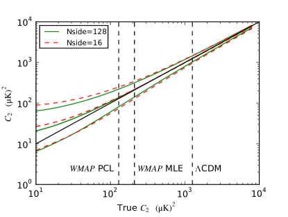
Figure 12: The same as Fig. 10 now comparing the weighted harmonic coefficient estimator (12) for $\textsc{Nside}=128$ as the green, solid lines and $\textsc{Nside}=16$ as the red, dashed lines without smoothing the map prior to reconstruction. Since there is no smoothing, the results do not depend on the contents of the masked galactic region. We see that the reconstruction without smoothing is unbiased for most of the $C_{2}$ range, however see Sec. 3.6 for a discussion of its inapplicability to real data.

3.6 Reconstructing Without Smoothing

The reconstruction of the $a_{2m}$ without smoothing showed that for $\textsc{Nside}=128$ the reconstruction was unbiased (Fig. 1) but for $\textsc{Nside}=16$ there was a resolution dependent bias (Fig. 2). Calculating the weighted harmonic coefficient estimator (12) from these realisations produces the results in Fig. 12. At first glance these results are surprising and encouraging. The green, solid lines for $\textsc{Nside}=128$ and red, dashed lines for $\textsc{Nside}=16$ nearly overlap and the central value very closely follows the true value. This is surprising since the $a_{2m}$ at $\textsc{Nside}=16$ are biased and have smaller variance than the corresponding $\textsc{Nside}=128$ (see Figs. 1 and 2). Even so, when combined to determine $C_{2}$ these differences average out and lead to nearly identical predictions.

Based on Fig. 12 we may think we have solved the reconstruction problem; just reconstruct using the optimal, unbiased $C_{\ell}$ estimator (12) without smoothing! Unfortunately we cannot draw this conclusion from the results presented here. Recall that the reconstructions have been performed on noise-free, pure CMB maps. Real maps contain noise and potentially residual, unmasked foregrounds. In particular uncorrected, diffuse foregrounds are known to contaminate the low-$\ell$ reconstruction (Naselsky et al., 2008). A careful study of the issues faced when applying the reconstruction to real data is beyond the scope of this work and will be reserved for future study. However, naive application of this method to real data yields highly biased reconstructions.

3.7 $\mn@boldsymbol{S_{1/2}}$ Estimator

The study of the $S_{1/2}$ statistic is a large project in its own right and will not be pursued in detail here. Our Universe as encoded in the ILC map contains a somewhat small full-sky $S_{1/2}$ and an extremely small cut sky $S_{1/2}$. If we are to perform such a statistical study of $S_{1/2}$ we could enforce this structure, that is, only choose skies that have somewhat low full-sky and very low cut-sky $S_{1/2}$ values. Alternatively we could choose from an ensemble based on the best-fitting $\Lambda$CDM model. In the latter case it has already been shown that the ILC map is a rare realisation, unlikely at the $99.975\%$ level (Copi et al., 2009). The assumptions made in any study will determine the statistical questions that can be asked. Conversely, the statistical questions asked will implicitly contain the assumptions imposed.

In Table 1 we show the $S_{1/2}$ for the ILC map calculated from (22) under various assumptions. Note that these values all contain the bias discussed in Sec. 2.5 as is standard in the literature. Shown in the table are the values calculated for the full sky and for the partial sky where the KQ75y7 mask is employed to cut out the Galactic region. The cut-sky results are calculated using the pixel based estimator of SpICE and the optimal, unbiased $C_{\ell}$ estimator (12) from reconstructed maps at $\textsc{Nside}=128$ and $\textsc{Nside}=16$. Further, the results are shown for different map processing, including no processing (the unsmoothed entry where the map has only been degraded as required for the reconstruction), employing a $10\degr$ Gaussian smoothing, and filling the Galactic region with a realisation that has the same power in each $\ell$-mode as the region outside the mask but with the phases randomised.

The results in Table 1 are consistent with what we have found for the $C_{\ell}$ reconstructions. For the unsmoothed map the full-sky and pixel based estimators calculated at $\textsc{Nside}=128$ show the usual result, the large discrepancy between the full and cut-sky values. This holds true for the smoothed map also. Further, the reconstructed values show the large discrepancy between the unsmoothed and smoothed maps (see, for example, Figs. 2 and 4). We also see that the reconstructed values are systematically larger than the pixel based estimator showing that the reconstruction is more sensitive to leakage for information from inside the masked region. Finally the last line of the table shows the expected behaviour for a map where the full sky has power consistent with that from the cut-sky. Notice that of the cut-sky pixel-based results are consistent with each other since information leakage is unimportant. The small difference between the $\textsc{Nside}=128$ and $\textsc{Nside}=16$ reconstructions shows the residual sensitivity on resolution.

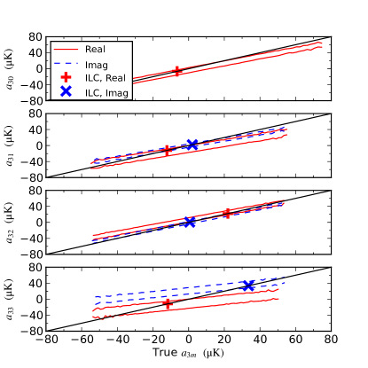
Figure 13: The $95$ and $5$ percentile lines for the $a_{3m}$ reconstructed from the pixels outside the KQ75y7 mask at $\textsc{Nside}=128$ (and thus $\ell_{\mathrm{max}}=514$) of $\Lambda$CDM realisations with $C_{2}=100\;\mathrm{(\mathrm{\mu K})^{2}}$ and the masked region filled in with the ILC map prior to smoothing and rescaling, as discussed in the text. The red, solid lines are for the real part of the $a_{3m}$ and the blue, dashed lines are for the imaginary part. The black, solid line shows the expected result for a perfect reconstruction. We clearly see the reconstructed $a_{3m}$ are not unbiased. Now the bias is most prominent for $a_{33}$, the octopole mode with all its extrema within the Galactic plane. This figure should be compared to Fig. 5.

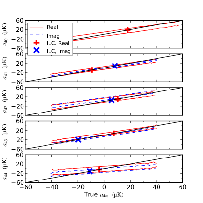
Figure 14: The same as Fig. 13 now for $\ell=4$.

3.8 Higher Multipoles

In this work we have focused on how data handling affects the reconstruction of the quadrupole. The quadrupole serves as an example of the general behaviour. As show in Figs. 13 and 14 we see the same results for $\ell=3$ and $\ell=4$. These figures were generated from the same realisations employed in making Fig. 5. Again we see that the reconstruction is biased toward the values from the ILC map.

4 Conclusions

It has been argued that the large-angle CMB can be reliably reconstructed from partial-sky data and that when this is done the lack of large-angle correlation is not significantly deviant from the expectation (Efstathiou et al., 2010). At first glance the argument appears sound. The large-angle modes extend over large fractions of the sky, thus knowing their values on one region of the sky allows us to extrapolate them into the masked regions. However, in practise and under close scrutiny this argument fails. Implicit assumptions built in to the reconstruction process enforce agreement between the reconstruction and the previously constructed full sky (the ILC map in this case) through mixing of information from inside the masked region to that outside. Due to this the reconstruction has no value independent of the original full-sky map. It neither confirms nor denies the validity of that map.

To study the large-angle CMB a choice must be made on what data to take as a fair representation of the CMB sky One choice is to accept a cleaned, full-sky map, such as the ILC map produced by WMAP, to accurately represent the primordial CMB sky. In this case the full-sky map may be analysed with no reconstruction required. In Copi et al. (2009) and in this work, however, we have taken the region outside the Galaxy as defined by the WMAP KQ75y7 mask to be a fair representation. We have shown that the large-angle CMB can be reconstructed using unbiased estimators for the $a_{\ell m}$ and $C_{\ell}$, however the standard approach requires processing the original map by degrading and smoothing it. Unfortunately it is precisely the smoothing process that mixes the region we have taken as a fair representation of the CMB with the region we are trying to exclude. When the excluded region has the same statistical properties as the region we are including then no biases are introduced. On the other hand, when, as is the case with the ILC map, the properties are significantly different the reconstruction is biased to agree with the full map. This is not surprising. Through this process one is trusting the full-sky map, mixing information from it into the rest of the sky, then reconstructing it. This is a circular process and is unnecessary. If the full-sky map is already trusted then there is no point in performing a reconstruction to produce a poorer version of the original map.

The important point is that even in principle reconstructing following the standard approach leads to biased results unless the full-sky CMB is already known. We have shown for noise free, pure CMB maps that smoothing mixes information and biases the results. When applied to real data the problems only get worse. Encouragingly we also found that in principle reconstructing without smoothing leads to unbiased results. Unfortunately, directly applying this to real data with noise and residual, unmasked foregrounds yields highly biased reconstructions requiring further care to apply this method successfully to real-world CMB.

Overall the question of how to perform an unbiased reconstruction of the full large angle CMB sky remains an interesting one. Previous work (Bielewicz et al., 2004; Naselsky et al., 2008; Liu & Li, 2009; Aurich & Lustig, 2010) has shown that contamination significantly affects the reconstruction of the large angle multipole moments. Aurich & Lustig (2010) studied the case most similar to that considered in this work. They showed that smoothing of full sky map leaks information from the pixels not used in the reconstruction (those in a mask) to the pixels that will be used. In this work we have extended their result and shown how a reconstruction such as that performed by Efstathiou et al. (2010) is biased due to this leakage of information. This shows the fundamental problem with trying to reconstruct the full sky from a partial sky.

Fortunately large-angle CMB studies are not dependent on reconstructed full-sky maps. The partial sky when used consistently (see Copi et al. 2009, for example) has been shown to be a robust representation of the large scale CMB by Aurich & Lustig (2010) and in this work. Despite the fact that such an approach is suboptimal in the sense that the inferred $C_{\ell}$ do not have the smallest possible variance, it is far less biased than the ‘optimal’ $C_{\ell}$ inferred through the maximum-likelihood reconstruction. More robust statements about the large-angle CMB behaviour may therefore be made with the partial sky pixel-based $C_{\ell}$.

We conclude that the lack of large-angle correlation, particularly on the region of the sky outside the Galaxy, remains a matter of serious concern.

Appendix A Reconstructing at High Resolution

Computationally the time and memory intensive step in reconstructing $a_{\ell m}$ and $C_{\ell}$ from our estimators (7) and (12) is the inversion of the covariance matrix, C. Fortunately this step only needs to be performed once for each choice of resolution, Nside, and mask.

The covariance matrix is of size $N_{\mathrm{pix}}\times N_{\mathrm{pix}}$ where the number of pixels is given by $12(\textsc{Nside})^{2}$ and the size of C scales as $(\textsc{Nside})^{4}$. An increase in resolution by one step, $\textsc{Nside}\rightarrow 2\textsc{Nside}$, increases the size of C by a factor of $16$. Working with cut skies does not appreciably reduce this, even the largest mask, KQ75y7, only cuts out $25$–$30$ percent of the pixels. Resolutions of $\textsc{Nside}=32$ or perhaps even $\textsc{Nside}=64$ are attainable on a desktop computer. Fortunately we never need to store the full $\textbf{{C}}^{-1}$ and can calculate the elements of C as required instead of storing them.

In our estimators all the matrices that we encounter, except for $\textbf{{C}}^{-1}$, are of size $N_{\ell}\times N_{\mathrm{pix}}$ or smaller. Here $N_{\ell}=(\ell_{\mathrm{recon}}+1)^{2}$. Even for $\textsc{Nside}=512$ and $\ell_{\mathrm{recon}}=10$ these matrices only require about $3\;\mathrm{GB}$ of storage at double precision. Further we see that only the matrix

$$\textbf{{M}}\equiv\textbf{{C}}^{-1}\textbf{{Y}}$$ (25)

is ever required (see Eqs. 7 and 8).

To compute M we note that it satisfies the set of linear equations

$$\textbf{{C}}\textbf{{M}}=\textbf{{C}}\textbf{{C}}^{-1}\textbf{{Y}}=\textbf{{Y}}.$$ (26)

Solving such a set of equations is a standard problem in computational linear algebra. A covariance matrix is symmetric and positive-definite so it may be factored with a Cholesky decomposition (Press et al., 1992)

$$\textbf{{C}}=\textbf{{L}}{\textbf{{L}}}^{\mathsf{T}},$$ (27)

where L is a lower triangular matrix. Our problem then becomes solving

$$\textbf{{L}}({\textbf{{L}}}^{\mathsf{T}}\textbf{{M}})\equiv\textbf{{L}}\textbf{{z}}=\textbf{{Y}}.$$ (28)

This can be solved in two steps using backward substitution on $\textbf{{L}}\textbf{{z}}=\textbf{{Y}}$ to find z followed by forward substitution on ${\textbf{{L}}}^{\mathsf{T}}\textbf{{M}}=\textbf{{z}}$ to find M.

At this point we are left with computing L. Approximately half of this matrix is zero so only half of it needs to be stored (of course the same is true of C since it is symmetric). Unfortunately this cannot be further reduced and this provides the limiting factor in determining the resolution at which we can work. For $\textsc{Nside}=128$ and $\ell_{\mathrm{recon}}=10$ the matrix L is approximately $70\;\mathrm{GB}$ in size. Improving resolution to $\textsc{Nside}=256$ increases the required storage to over $1\;\mathrm{TB}$. This is what has limited our work to $\textsc{Nside}=128$. Straight forward, numerically stable algorithms exist for calculating L (see Press et al. 1992, for example). Though this is a time consuming step once M is calculated the rest follows quickly.

References

- Afshordi et al. (2009) Afshordi N., Geshnizjani G., Khoury J., 2009, JCAP, 8, 30
- Aurich & Lustig (2010) Aurich R., Lustig S., 2010, MNRAS, 1650
- Bennett et al. (1996) Bennett C.L. et al., 1996, ApJ, 464, L1
- Bennett et al. (2003) Bennett C.L. et al., 2003, ApJS, 148, 1
- Bennett et al. (2011) Bennett C.L. et al., 2011, ApJS, 192, 17
- Bielewicz et al. (2004) Bielewicz P., Górski K.M., Banday A.J., 2004, MNRAS, 355, 1283
- Chon et al. (2004) Chon G., Challinor A., Prunet S., Hivon E., Szapudi I., 2004, MNRAS, 350, 914
- Copi et al. (2006) Copi C.J., Huterer D., Schwarz D.J., Starkman G.D., 2006, MNRAS, 367, 79
- Copi et al. (2007) Copi C.J., Huterer D., Schwarz D.J., Starkman G.D., 2007, Phys. Rev. D, 75, 023507
- Copi et al. (2009) Copi C.J., Huterer D., Schwarz D.J., Starkman G.D., 2009, MNRAS, 399, 295
- Copi et al. (2010) Copi C.J., Huterer D., Schwarz D.J., Starkman G.D., 2010, Advances in Astronomy, 2010, 78
- de Oliveira-Costa & Tegmark (2006) de Oliveira-Costa A., Tegmark M., 2006, Phys. Rev. D, 74, 023005
- de Oliveira-Costa et al. (2004) de Oliveira-Costa A., Tegmark M., Zaldarriaga M., Hamilton A., 2004, Phys. Rev. D, 69, 063516
- Efstathiou (2004) Efstathiou G., 2004, MNRAS, 349, 603
- Efstathiou et al. (2010) Efstathiou G., Ma Y., Hanson D., 2010, MNRAS, 407, 2530
- Eriksen et al. (2004a) Eriksen H.K., Hansen F.K., Banday A.J., Górski K.M., Lilje P.B., 2004a, ApJ, 605, 14
- Eriksen et al. (2004b) Eriksen H.K., Hansen F.K., Banday A.J., Górski K.M., Lilje P.B., 2004b, ApJ, 609, 1198
- Górski et al. (2005) Górski K.M., Hivon E., Banday A.J., Wandelt B.D., Hansen F.K., Reinecke M., Bartelmann M., 2005, ApJ, 622, 759
- Hajian (2007) Hajian A., 2007, astro-ph/0702723
- Hansen et al. (2009) Hansen F.K., Banday A.J., Górski K.M., Eriksen H.K., Lilje P.B., 2009, ApJ, 704, 1448
- Kim & Naselsky (2010a) Kim J., Naselsky P., 2010a, ApJ, 714, L265
- Kim & Naselsky (2010b) Kim J., Naselsky P., 2010b, Phys. Rev. D, 82, 063002
- Kim & Naselsky (2010c) Kim J., Naselsky P., 2010c, preprint (arXiv:1011.0377)
- Kim & Naselsky (2010d) Kim J., Naselsky P., 2010d, ApJ, 724, L217
- Land & Magueijo (2005) Land K., Magueijo J., 2005, MNRAS, 362, 838
- Larson et al. (2011) Larson D. et al., 2011, ApJS, 192, 16
- Liu & Li (2009) Liu H., Li T., 2009, Science in China G: Physics and Astronomy, 52, 804
- Naselsky et al. (2008) Naselsky P.D., Verkhodanov O.V., Nielsen M.T.B., 2008, Astrophysical Bulletin, 63, 216
- Pontzen & Peiris (2010) Pontzen A., Peiris H.V., 2010, Phys. Rev. D, 81, 103008
- Press et al. (1992) Press W.H., Teukolsky S.A., Vetterling W.T., Flannery B.P., 1992, Numerical Recipes in C, 2nd ed., Cambridge University Press, Cambridge
- Sarkar et al. (2011) Sarkar D., Huterer D., Copi C.J., Starkman G.D., Schwarz D.J., 2011, Astropart. Phys., 34, 591
- Schwarz et al. (2004) Schwarz D.J., Starkman G.D., Huterer D., Copi C.J., 2004, Phys. Rev. Lett., 93, 221301
- Slosar & Seljak (2004) Slosar A., Seljak U., 2004, Phys. Rev. D, 70, 083002
- Spergel et al. (2003) Spergel D.N. et al., 2003, ApJS, 148, 175
- Tegmark (1997) Tegmark M., 1997, Phys. Rev. D, 55, 5895