Product of Ginibre matrices: Fuss-Catalan and Raney distributions

Abstract

Squared singular values of a product of $s$ square random Ginibre matrices are asymptotically characterized by probability distributions $P_{s}(x)$, such that their moments are equal to the Fuss–Catalan numbers or order $s$. We find a representation of the Fuss–Catalan distributions $P_{s}(x)$ in terms of a combination of $s$ hypergeometric functions of the type ${}_{s}F_{s-1}$. The explicit formula derived here is exact for an arbitrary positive integer $s$ and for $s=1$ it reduces to the Marchenko–Pastur distribution. Using similar techniques, involving Mellin transform and the Meijer $G$–function, we find exact expressions for the Raney probability distributions, the moments of which are given by a two parameter generalization of the Fuss-Catalan numbers. These distributions can also be considered as a two parameter generalization of the Wigner semicircle law.

I Introduction

Random matrices of various ensembles find numerous applications in several fields of statistical physics. In the general class of non-hermitian random matrices an important role is played by the Ginibre ensemble Gi65 . A matrix $G$ of size $N$ of such an ensemble consists of $N^{2}$ independent random complex numbers, drawn according to the Gaussian distribution with zero mean and a fixed variance Me04 ; Fo10 . Such matrices are used to describe non-unitary dynamics of chaotic systems and open quantum systems Ha10 . This ensemble of random matrices can also be used to analyze the human EEG data Se03 , for telecommunication applications based on the scattering of electromagnetic waves on random obstacles TV04 , or in mathematical finances to describe correlation matrices of various stocks BP ; BJN03 .

The spectrum of a non-Hermitian matrix $G$ belongs to the complex plane. Spectral density of random matrices of the suitably normalized Ginibre ensemble is described by the Girko circular law Gi84 , as in the limit $N\to\infty$ it covers uniformly the unit disk. The random matrix $W=GG^{\dagger}$, called a Wishart matrix, is positive. Hence its eigenvalues $\lambda_{i}$, $i=1,\dots,N$, are real and non-negative. Introducing a rescaled eigenvalue, $x=N\lambda$ one can show that in the limit of the large matrix size the spectral density $P(x)$ converges to the Marchenko–Pastur (MP) distribution MP67 .

In general, products of random matrices are a subject of an intensive research for many years CPV93 . Recent studies on products of Ginibre matrices concern multiplicative diffusion processes GJJN03 , correlation matrices used in macroeconomic time series BLMM07 , a random matrix approach to quantum chromodynamics Os04 and lattice gauge field theories LNW08 . Properties of the complex spectra of products of random Ginibre matrices were recently analyzed in BJW10 .

It is also interesting to study singular values of a product of $s$ independent Ginibre matrices, $X=G_{1}\cdots G_{s}$. Note that a squared singular value of the product $X$ equals the corresponding eigenvalue of the Wishart like matrix $W=XX^{\dagger}$. For $s=2$, positive random matrices of the form $W_{2}=G_{1}G_{2}(G_{1}G_{2})^{\dagger}$ found their applications in finances BLMM07 . Matrices of the form $W_{s}=G_{1}\cdots G_{s}(G_{1}\cdots G_{s})^{\dagger}$ for an arbitrary $s$ were used to describe random quantum states associated with certain graphs CNZ10 and quantum states obtained by orthogonal measurements in a product of maximally entangled bases ZPNC10 .

The corresponding asymptotic level density distribution $P_{s}(x)$ is called Fuss-Catalan distribution of order $s$, since its moments are given armstrong ; Ml10 ; banica-etal by the Fuss-Catalan numbers GKP ; Ko08 , (also called Fuss numbers PS00 ). Strangely enough, the Fuss-Catalan numbers generalize the Catalan numbers, although the work of Fuß Fu791 was done much earlier then the contribution of Catalan Ca838 . The Catalan number can be defined as a number of different bracketing of a product of $n+1$ numbers, or the number of possible $n$ folding of a map which contains $n+1$ pages in a row Ko68 .

The Fuss–Catalan distribution describes asymptotically statistics of singular values of the $s$–th power of random Ginibre matrices. This result obtained recently by Alexeev et al. AGT10 was derived by estimating the moments of the distribution of squared singular values of a power $G^{s}$ of a random matrix and showing that these moments converge asymptotically to the Fuss–Catalan numbers. This is true under rather weak assumptions: all entries of the matrix $G$ are independent random variables characterized by the zero mean, variance set to unity and finite fourth moment.

The Fuss–Catalan distribution can be considered as a generalization of the MP distribution, which is obtained for $s=1$. Moreover, the distribution $P_{s}(x)$ belongs to the class of free Meixner measures bozejko-bryc , and in terms of free probability theory it appears as the free multiplicative convolution product of $s$ copies of the MP distribution banica-etal ; BG09 , which is written as $P_{s}(x)=[P_{1}(x)]^{\boxtimes s}$.

An explicit form in the case $s=2$ was derived in PS01 in context of construction of generalized coherent states from combinatorial sequences. The spectral distribution of $P_{s}(x)$ for a product of an arbitrary number of $s$ random Ginibre matrices was recently analyzed by Burda et al. BJLNS10 also in the general case of rectangular matrices. The distribution was expressed as a solution of a polynomial equation and it was conjectured that the finite size effects can be described by a simple multiplicative correction. Another recent work of Liu at al. LSW10 provides an integral representation of the distribution $P_{s}(x)$ derived in the case of $s$ square matrices of size $N$, which is assumed to be large. However, these recent contributions do not provide an explicit form of the distribution $P_{s}(x)$.

The aim of this note is to derive exact and explicit formulae for the Fuss-Catalan distribution $P_{s}(x)$, which can be represented as a combination of $s$ hypergeometric functions. The derivation is presented in Sec. II, while some auxiliary information on special functions and the proof of positivity of $P_{s}(x)$ are provided in Appendices A and B, respectively. In section III we discuss a certain two-parameters generalization of Fuss-Catalan numbers. As these numbers quantify generalized Raney sequences GKP , the corresponding probability measures $W_{p,r}(x)$ will be called Raney distributions. As special cases they include Marchenko–Pastur distribution, Fuss–Catalan distributions and the Wigner semicircle law. We find exact expressions for Raney distributions corresponding to integer parameter values in the general case and provide explicit formulae in the simplest cases of small values of the integer parameters $1\leq r\leq p$.

II Fuss–Catalan distributions

For any integer number $s$ one can use the binomial symbol to define a sequence of integers denoted by $FC_{s}(n)$,

$$FC_{s}(n):=\frac{1}{sn+1}\binom{sn+n}{n}\ .$$ (1)

Here $n=0,1,\dots$, while $s=1,2,\dots$, and these numbers are called the Fuss–Catalan numbers of order $s$ GKP .

We enumerate some of these sequences below for $n=0,\dots,7$:

$$FC_{1}(n) = 1,1,2,5,14,42,132,427,\dots$$

$$FC_{2}(n) = 1,1,3,12,55,273,1428,7752,\dots$$

$$FC_{3}(n) = 1,1,4,22,140,969,7084,53820,\dots$$

$$FC_{4}(n) = 1,1,5,35,285,2530,23751,231880,\dots\;.$$

The above sequences are contained in the Online Encyclopedia of Integer Sequences (OEIS) Sloane under the labels (A000108), (A001724), (A002293) and (A002294), respectively. These sequences can be considered as a generalization of the sequence $FC_{1}(n)$, which consists of Catalan numbers, $C(n)=\frac{1}{n+1}\binom{2n}{n}$.

We are going to show that for any given $s$ there exists a density distribution $P_{s}(x)$, which satisfies

$$\int_{0}^{K_{s}}x^{n}P_{s}(x)dx=FC_{s}(n),\ \ n=0,1,\dots$$ (2)

where

$$K_{s}:=(s+1)^{s+1}/s^{s}\;.$$ (3)

In other words we are looking for a positive density $P_{s}(x)$ which satisfies the above infinite system of equations. As the density turns out to be defined in a finite segment $[0,K_{s}]$, the solution of this Hausdorff moment problem Ak65 associated with the Fuss-Catalan numbers is unique. An explicit proof of positivity of $P_{s}(x)$ is provided in Appendix B.

We employ the method of the inverse Mellin transform, which was previously used to construct explicit solutions of the Hausdorff moment problem KPS01 ; GPHDS and to derive explicit form of the Lévy–stable distributions PG10 . The Mellin transform ${\cal M}$ of a function $f(x)$ and its inverse ${\cal M}^{-1}$ are defined by a pair of equations

$$f^{*}(\sigma):=\;{\cal M}[f(x);\sigma]=\int_{0}^{\infty}x^{\sigma-1}f(x)dx$$ (4)

and

$$f(x):=\;{\cal M}^{-1}[f^{*}(\sigma);x]=\frac{1}{2\pi i}\int_{c-i\infty}^{c+i\infty}x^{-\sigma}f^{*}(\sigma)d\sigma,$$ (5)

with complex $\sigma$. In (5) this variable is integrated over a vertical line in the complex plane FGD95 . For discussion concerning the role of $c$, see (FGD95 ; PBM98 ; Lu69 ). Therefore the solution of Eq. (2) can be obtained by extending integer variable $n$ to complex $\sigma$ by a substitution $n\to\sigma-1$. The desired form of the distribution $P_{s}(x)$ can be formally written as an inverse Mellin transform,

$$P_{s}(x)\ =\ {\cal M}^{-1}[FC_{s}(\sigma);x]\ .$$ (6)

To find such a transform we will bring the Fuss-Catalan numbers into a more suitable form. Representing the binomial symbol in (1) by the ratio of Euler’s gamma function one obtains

$$FC_{s}(\sigma)=\frac{\Gamma\bigl{[}(s+1)\bigl{(}\sigma-\frac{s}{s+1}\bigr{)}\bigr{]}}{\Gamma\bigl{[}s\bigl{(}\sigma-\frac{s-2}{s}\bigr{)}\bigr{]}\;\Gamma(\sigma)}\ .$$ (7)

After applying twice the Gauss–Legendre formula (34) for multiplication of the argument of the gamma function one arrives at

$$FC_{s}(\sigma) = \frac{1}{\sqrt{2\pi}}\Bigl{[}\frac{(s+1)^{s+1}}{s^{s}}\Bigr{]}^{\sigma}\times$$ (8)

$$\times \;\frac{s^{s-3/2}}{(s+1)^{s+1/2}}\;\Bigl{[}\prod_{j=0}^{s-1}\frac{\Gamma\bigl{(}\sigma+\frac{j-s}{s+1}\bigr{)}}{\Gamma\bigl{(}\sigma+\frac{2+j-s}{s}\bigr{)}}\Bigr{]}.$$

Obtaining the above form of the FC numbers, in which a ratio of products of the gamma functions of a shifted argument appears, is a key step of our reasoning. It allows us to represent the inverse Mellin transform of Eq. (8) as a certain special function. To see this recall that the Meijer $G$–function of the argument $z$ can be defined by the inverse Mellin transform PBM98 :

$$G_{p,q}^{m,n}\Bigl{(}z\;\bigl{|}\;{\stackrel{{\scriptstyle\scriptstyle\alpha_{1}\cdots\alpha_{p}}}{{\scriptstyle\beta_{1}\cdots\beta_{q}}}}\Bigr{)}=$$ (9)

$$={\cal M}^{-1}\Bigl{[}\frac{\prod_{j=1}^{m}\Gamma(\beta_{j}+\sigma)\prod_{j=1}^{n}\Gamma(1-\alpha_{j}-\sigma)}{\prod_{j=m+1}^{q}\Gamma(1-\beta_{j}-\sigma)\prod_{j=n+1}^{p}\Gamma(\alpha_{j}+\sigma)};\;z\Bigr{]}.$$

This definition involves four lists of parameters, which can be represented by $p$ complex numbers $\alpha_{j}$ and other $q$ complex numbers $\beta_{j}$. Integers numbers $p$ and $q$ can be equal zero and it s is assumed that $0\leq m\leq q$ and $0\leq n\leq p$, so that possibly empty products in this form are taken to be equal to unity. A detailed description of the integration contours of the Mellin transform (9), general properties of the Meijer functions and its special cases can be found in PBM98 .

Figure 1: (Color online) Marchenko–Pastur distribution $P_{1}(x)$ compared with the Fuss–Catalan distribution $P_{2}(x)$. The singularity at $x\to 0$ is of the type $P_{s}(x)\sim x^{-s/(s+1)}$.

Figure 2: (Color online) Fuss–Catalan distributions $P_{s}(x)$ plotted for parameter $s$ equal to $3,4,5$ and $6$ are supported on the interval $[0,(s+1)^{s+1}/s^{s}]$. To show behaviour at the right side of the support the figure is plotted for $x\geq 5$.

Direct comparison of expression (8) for the Fuss Catalan numbers and the Mellin transform as the Meijer $G$–function (9) allows us to represent the Fuss-Catalan distribution $P_{s}(x)$ by a Meijer $G$–function,

$$P_{s}(x)=\frac{1}{\sqrt{2\pi}}\frac{s^{s-3/2}}{(s+1)^{s+1/2}}\;G_{s,s}^{s,0}\Bigl{(}z\;\bigl{|}\;{\stackrel{{\scriptstyle\scriptstyle\alpha_{1}\cdots\alpha_{p}}}{{\scriptstyle\beta_{1}\cdots\beta_{q}}}}\Bigr{)}$$ (10)

of the argument $z=xs^{s}(s+1)^{-(s+1)}$. Looking at the range of the parameter $j$ in (8) we see that the numbers of parameters of the Meijer $G$–function have to be set to $n=0$, $p=s$ and $m=q=s$. Hence this function involves $2s$ parameters, which read $\alpha_{j}=(1+j-s)/s$ and $\beta_{j}=(j-1-s)/(s+1)$ for $j=1,\dots,s$.

As there are only two products of gamma functions in (8), in contrast to four in (9), which is equivalent to setting $n=0$ and $m=q$, a further simplification of the above formula is possible. In this very case the Meijer $G$–function can be written as a combination of hypergeometric functions of the same argument $z$ – see Eq. (5.2.11) p. 146 of Lu69 .

Let ${}_{p}F_{q}\Bigl{(}\bigl{[}\{a_{j}\}_{j=1}^{p}\bigr{]},\;\bigl{[}\{b_{j}\}_{j=1}^{q}\bigr{]};\;x\Bigr{)}$ denote the hypergeometric function MOT of the type ${}_{p}F_{q}$ with $p$ ’upper’ parameters $a_{j}$ and $q$ ’lower’ parameters $b_{j}$ of the argument $x$. The symbol $\{a_{i}\}_{i=1}^{r}$ represents the list of $r$ elements, $a_{1},\dots a_{r}$. Then formula (10) for the Fuss–Catalan distribution can be rewritten as

$$P_{s}(x)=\sum_{k=1}^{s}\Lambda_{k,s}\;x^{\frac{k}{s+1}-1}\;{}_{s}F_{s-1}\Bigl{(}\Bigl{[}\Bigl{\{}1-\frac{1+j}{s}+\frac{k}{s+1}\Bigr{\}}_{j=1}^{s}\Bigr{]},\;\Bigl{[}\Bigl{\{}1+\frac{k-j}{s+1}\Bigr{\}}_{j=1}^{k-1},\Bigl{\{}1+\frac{k-j}{s+1}\Bigr{\}}_{j=k+1}^{s}\Bigr{]};\;\frac{s^{s}}{(s+1)^{s+1}}x\Bigr{)}\ .$$ (11)

where the coefficients $\Lambda_{k,s}$ read for $k=1,2,\dots,s$

$$\Lambda_{k,s}:=s^{-3/2}\sqrt{\frac{s+1}{2\pi}}\Bigl{(}\frac{s^{s/(s+1)}}{s+1}\Bigr{)}^{k}\ \frac{\Bigl{[}\prod_{j=1}^{k-1}\Gamma\bigl{(}\frac{j-k}{s+1}\bigr{)}\Bigr{]}\Bigl{[}\prod_{j=k+1}^{s}\Gamma\bigl{(}\frac{j-k}{s+1}\bigr{)}\Bigr{]}}{\prod_{j=1}^{s}\Gamma\bigl{(}\frac{j+1}{s}-\frac{k}{s+1}\bigr{)}}\ .$$ (12)

This formula, along with Eq.(22) below, constitutes the key result of the present note. It gives an exact result for the Fuss–Catalan distribution $P_{s}(x)$ for an arbitrary natural $s$. The FC distribution describes the density of squared singular values of a product of $s$ independent square Ginibre matrices in the limit of large matrix size.

The convergence conditions of the hypergeometric series ${}_{s}F_{s-1}$ immediately yield the support of $P_{s}(x)$ which is equal to $[0,(s+1)^{s+1}/s^{s}]$. For small values of $x$ the distribution behaves as $x^{-s/(s+1)}$. It is conforting to see that in the simplest case $s=1$ the above complicated form reduces indeed to the Marchenko–Pastur distribution,

$$P_{1}(x)=\frac{1}{\pi\sqrt{x}}\;{}_{1}F_{0}\Bigl{(}[-\frac{1}{2}],[\ ];\;\frac{1}{4}x\Bigr{)}=\frac{\sqrt{1-x/4}}{\pi\sqrt{x}}\;.$$ (13)

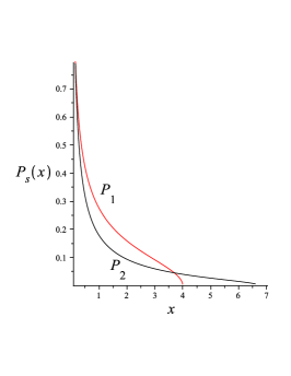
Furthermore, the distribution $P_{2}(x)$, shown in Fig. 1,

$$P_{2}(x)= \frac{\sqrt{3}}{2\pi x^{2/3}}\;{}_{2}F_{1}\Bigl{(}\bigl{[}-\frac{1}{6},\frac{1}{3}\bigr{]},\;\bigl{[}\frac{2}{3}\bigr{]};\;\frac{4}{27}x\Bigr{)}\ \ \ \ \ \ \ \$$ (14)

$$-\frac{\sqrt{3}}{6\pi x^{1/3}}\;{}_{2}F_{1}\Bigl{(}\bigl{[}\frac{1}{6},\frac{2}{3}\bigr{]},\;\bigl{[}\frac{4}{3}\bigr{]};\;\frac{4}{27}x\Bigr{)}$$

is equivalent to the form,

$$\!\!P_{2}(x)=\frac{\sqrt[3]{2}\sqrt{3}}{12\pi}\;\frac{\bigl{[}\sqrt[3]{2}\left(27+3\sqrt{81-12x}\right)^{\frac{2}{3}}-6\sqrt[3]{x}\bigr{]}}{x^{\frac{2}{3}}\left(27+3\sqrt{81-12x}\right)^{\frac{1}{3}}},$$ (15)

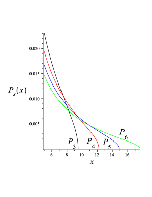
valid for $x\in[0,27/4]$ and obtained first in PS01 in context of construction of generalized coherent states from combinatorial sequences. The distribution $P_{3}(x)$, plotted in Fig. 2, is given by a sum of three terms,

$$P_{3}(x)=\!\! \frac{1}{\sqrt{2}\pi x^{3/4}}\;{}_{3}F_{2}\Bigl{(}\bigl{[}-\frac{1}{12},\frac{1}{4},\frac{7}{12}\bigr{]},\;\bigl{[}\frac{1}{2},\frac{3}{4}\bigr{]};\;\frac{27}{256}x\Bigr{)}\ \ \ \ \ \ \ \$$ (16)

$$\!\!-\frac{1}{4\pi x^{1/2}}\;{}_{3}F_{2}\Bigl{(}\bigl{[}\frac{1}{6},\frac{1}{2},\frac{5}{6}\bigr{]},\;\bigl{[}\frac{3}{4},\frac{5}{4}\bigr{]};\;\frac{27}{256}x\Bigr{)}\ \ \ \ \ \ \ \$$

$$\!\!-\frac{\sqrt{2}}{64\pi x^{1/4}}\;{}_{3}F_{2}\Bigl{(}\bigl{[}\frac{5}{12},\frac{3}{4},\frac{13}{12}\bigl{]},\;\bigl{[}\frac{5}{4},\frac{3}{2}\bigr{]};\;\frac{27}{256}x\Bigr{)}.$$

In Fig. 2 we present the Fuss–Catalan distributions $P_{s}(x)$ for $s=3,4,5$ and $6$.

III Raney distributions

The Fuss–Catalan numbers $FC_{s}(n)$ defined in (1) can be considered as a special cases of a larger family of sequences,

$$R_{p,r}(n):=\frac{r}{pn+r}\binom{pn+r}{n}$$ (17)

defined for $n=0,1,\dots$. Here $p$ and $r$ are treated as integer parameters, $p\geq 2$, $r=1,2,\dots$ . Setting $r=1$ and $p=s+1$ we have $\frac{1}{np+1}\binom{np+1}{n}=\frac{1}{n(p-1)+1}\binom{np}{n}$, so the numbers $R_{s+1,1}(n)$ are equal to $FC_{s}(n)$. Further relations involving the sequences $R_{p,r}(n)$ are

$$R_{p+1,p+1}(n)=FC_{p}(n+1),$$ (18)

and

$$R_{p,p}(n)=R_{p,1}(n+1),$$ (19)

which can be verified directly from their definitions (1) and (17).

The Raney lemma Ra60 implies that the number of the Raney sequences of order $p$ and length $pn+1$, for which all partial sums are positive, is given by the Fuss–Catalan numbers $FC_{p-1}(n)=R_{p,1}(n)$. Furthermore, as the number of positive generalized Raney sequences is equal to $R_{p,r}(n)$ GKP we will refer to $R_{p,r}(n)$ defined in (17) as Raney numbers. These numbers appear as coefficients in a generalized binomial series GKP . Some representative examples of sequences $R_{p,r}(n)$, for $n=0,1,\dots,7$ are quoted below together with their OEIS labels Sloane ,

$$R_{4,2}(n) = 1,2,9,52,340,2394,17710,135720,...(A069271)$$

$$R_{5,2}(n) = 1,2,11,80,665,5980,56637,556512,...(A118969),$$

whereas two following sequences are not represented in OEIS:

$$R_{4,5}(n) = 1,5,30,200,1425,10626,81900,647280,...\;,$$

$$R_{6,3}(n) = 1,3,21,190,1950,21576,250971,3025308,...\;.$$

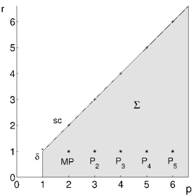
In a recent work Młotkowski Ml10 has shown that the sequence (17) describes moments of a probability measure $\mu_{p,r}$ with a compact support contained in $[0,\infty)$, if point $(r,p)$ which determines parameters of the Raney numbers belongs to the set $\Sigma$ defined by inequalities $p\geq 0$ and $0<r\leq p$. Note that the point $(1,1)$ implies a constant sequence of moments, $R_{1,1}(n)=1$, which represents a singular, Dirac delta measure, $\mu_{1,1}=\delta(x-1)$.

In the case the measure $\mu_{p,r}$ is represented by a density we will denote it by $W_{p,r}(x)$. Setting $r$ to one one gets the Fuss–Catalan numbers, which implies that $W_{2,1}(x)$ represents the Marchenko–Pastur distribution, while $W_{s+1,1}(x)$ reduces to the Fuss–Catalan probability density $P_{s}(x)$.

In general parameters $p$ and $r$ can be taken to be real and then the moments of the measure are expressed by the gamma functions,

$$\int x^{n}\mu_{p,r}(x)dx=\frac{r}{np+r}\frac{\Gamma(np+r+1)}{\Gamma(n+1)\Gamma(np+r-n+1)},$$ (20)

where the integration covers entire support of the measure $\mu_{p,r}$. For $1\leq r\leq p$ the distribution $W_{p,r}(x)$ is a positive function, see Ml10 and Appendix B.

The corresponding distribution $W_{p,r}(x)$ can be written implicitly by its $S$-transform, which allowed Młotkowski to establish relations between various Raney distributions Ml10 , listed in Appendix C. For a precise definition of the $S$–transform (or the free multiplicative transform) see Eq. 4.9 in Ml10 . In spite of these concrete results an explicit form of the Raney distribution $W_{p,r}(x)$ has not appeared in the literature so far.

Making use of the inverse Mellin transform and the Meijer function we can generalize results of the previous section and obtain explicit expressions for the Raney distributions $W_{p,r}(x)$, which correspond to integer values of the parameters $p$ and $r$.

Repeating steps analogous to Eqs.(7) – (10) we can represent distribution $W_{p,r}(x)$ in terms of the Meijer $G$–function. The explicit expression generalizing Eq.(10) reads

$$W_{p,r}(x)=\frac{r}{\sqrt{2\pi}}\frac{p^{r-p-1/2}}{(p-1)^{r-p+3/2}}\;G_{p,p}^{p,0}\Bigl{(}z\;\bigl{|}\;{\stackrel{{\scriptstyle\scriptstyle\alpha_{1}\cdots\alpha_{p}}}{{\scriptstyle\beta_{1}\cdots\beta_{q}}}}\Bigr{)},$$ (21)

where the argument of the function is $z=x(p-1)^{p-1}/p^{p}$, while its parameters are $\alpha_{1}=0$, $\alpha_{j}=(r-p+j)/(p-1)$ for $j=2,\dots,p$ and $\beta_{j}=(r-p-1+j)/p$ for $j=1,\dots,p$. In analogy to (11) this relation can be represented by the following sum consisting of of $p$ terms:

$$\!\!W_{p,r}(x)=\sum_{j=1}^{p}\Omega(p,r;j)x^{\frac{r-1+j}{p}-1}\;{}_{p}F_{p-1}\Bigl{(}\Bigl{[}1+\beta_{j},\Bigl{\{}1+\beta_{j}-\alpha_{i}\Bigr{\}}_{i=2}^{p}\Bigr{]},\;\Bigl{[}\Bigl{\{}1+\frac{j-i_{2}}{p}\Bigr{\}}_{i_{2}=1}^{j-1},\Bigl{\{}1+\frac{j-i_{3}}{p}\Bigr{\}}_{i_{3}=j+1}^{p}\Bigr{]};\;\frac{(p-1)^{p-1}}{p^{p}}x\Bigr{)}\;,$$ (22)

where ${}_{p}F_{p-1}$ is the hypergeometric function and the numerical coefficients $\Omega(p,r;j)$, for $j=1,2,\dots,p$ read

$$\Omega(p,r;j):=\frac{r}{\sqrt{2\pi}}\frac{p^{r-p-1/2}}{(p-1)^{r-p+3/2}}\Bigl{(}\frac{(p-1)^{p-1}}{p^{p}}\Bigr{)}^{\frac{r-p-1+j}{p}}\;\frac{1}{\Gamma\bigl{(}\frac{p-r+1-j}{p}\bigr{)}}\;\frac{\Bigl{[}\prod_{i_{1}=1}^{j-1}\Gamma\bigl{(}\frac{i_{i}-j}{p}\bigr{)}\Bigr{]}\Bigl{[}\prod_{i_{2}=1}^{p-j}\Gamma\bigl{(}\frac{i_{2}}{p}\bigr{)}\Bigr{]}}{\prod_{i_{3}=2}^{p}\Gamma\bigl{(}\frac{r-p+i_{3}}{p-1}-\frac{r-p-1+j}{p}\bigr{)}}\ .$$ (23)

Convergence properties of the hypergeometric function imply that the Raney distribution $W_{p,r}(x)$ for integer values of its parameters is supported in the interval $[0,K_{p-1}]$, where $K_{s}$ is given in Eq. (3). Formula (22) implies that for $p>r$ the distribution $W_{p,r}(x)$ diplays a singularity for small $x$ of the type $x^{-(p-r)/p}$. For $p=r$ the ’diagonal’ Raney distributions behave for small arguments as $W_{p,p}(x)\sim x^{1/p}$.

It is helpful to add some clarifying remarks concerning the key formula (22). We draw attention to the fact that some simplifications will always appear for two reasons:

a) firstly, one parameter form the ’upper’ list of the parameters will be always equal to a parameter from the ’lower’ list. Consider, for instance, the case $p=4$ and $r=2$. Then the value of the first parameter in the ’upper’ list becomes $1+(j-3)/4$ and it cancels with the value of $i_{3}=3$ of the first sequence of the ’lower’ parameters. One can demonstrate that a similar cancellation effect takes place for any pair $(p,r)$. Therefore, the hypergeometric function ${}_{p}F_{p-1}$ in (22) effectively reduces to ${}_{p-1}F_{p-2}$.

b) secondly, we see from Eq.(23) that the coefficient $\Omega(p,r;j)$ vanishes for $j=p+1-r$, due to the presence of the first gamma function in denominator. Therefore the sum in Eq. (22) involves $(p-1)$ terms with different hypergeometric functions ${}_{p-1}F_{p-2}$. Then it can be explicitly verified that from the equality between the numbers $R_{s+1,1}(n)=FC_{s}(n)$, the corresponding equality between the probability distributions

$$W_{s+1,1}(x)\ =\ P_{s}(x)$$ (24)

follows. In particular the following identity between the coefficients holds, $\Omega(s+1,1;j)=\Lambda_{j,s}$, whose demonstration is rather tedious and will not be reproduced here.

With the two provisos explained under items a) and b) above, Eq.(22) will be used to obtain explicit forms of distributions $W_{p,r}(x)$ for small values of $r$ and $p$. In particular, the case $W_{2,2}(x)$ reduces to the celebrated semi-circular law Me04 :

$$\!W_{2,2}(x)=\frac{\sqrt{x}}{\pi}\;{}_{1}F_{0}\Bigl{(}[-\frac{1}{2}],[\ ];\;\frac{x}{4}\Bigr{)}=\frac{1}{2\pi}\sqrt{x(4-x)}.$$ (25)

The above semicircle is centered at $x=2$, while the Wigner semicircle centered at $x=0$ is used in random matrix theory to describe the asymptotic level density of random hermitian matrices form Gaussian ensembles Me04 ; Fo10 . The Raney distributions $W_{2,r}(x)$ are plotted in Fig. 3 for $r=1$ and $r=2$. For comparison we have also plotted the function $W_{2,3}(x)$ furnished by Eq. (22). According to the results of Młotkowski Ml10 and our Appendix B this function is not positive in its domain, so it does not represent a probability distribution. Here we obtain it explicitly.

Figure 3: (Color online) Raney distributions $W_{2,r}(x)$ with values of the parameter $r$ labeling each curve. For $r=1$ it reduces to Marchenko-Pastur distribution $P_{1}(x)$, while a semicircle law is obtained for $r=2$. For $r=3$ the function represented by dashed line is not positive, which is implied by $p<r$.

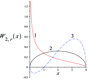
It is easy to observe that the above semicircle distribution is related with the Marchenko-Pastur distributions $P_{1}(x)$ by a relation $W_{2,2}(x)=xP_{1}(x)$. This is a special case of a more general relation involving the ”diagonal” Raney distributions with $r=p$ and Fuss-Catalan distribution,

$$W_{p,p}(x)=x\;W_{p,1}(x)=xP_{p-1}(x).$$ (26)

This result, established first in Ml10 , follows also naturally from Eqs.(21) and (22). Thus for $p=3$ one has

$$W_{3,1}(x)=P_{2}(x),\ \ {\rm and}\ \ W_{3,3}(x)=x\;P_{2}(x),$$ (27)

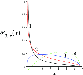
where the Fuss-Catalan distribution $P_{2}(x)$ is given in (14). Due to an equivalent expression (15) the distribution $W_{3,3}(x)$ can also be expressed in terms of elementary functions. The intermediate Raney distribution, corresponding to $r=2$,

$$W_{3,2}(x)= \frac{\sqrt{3}}{2\pi x^{1/3}}\;{}_{2}F_{1}\Bigl{(}\bigl{[}-\frac{1}{3},\frac{1}{6}\bigr{]},\;\bigl{[}\frac{1}{3}\bigr{]};\;\frac{4}{27}x\Bigr{)}\ \ \ \ \ \ \ \$$ (28)

$$-\frac{\sqrt{3}x^{1/3}}{18\pi}\;{}_{2}F_{1}\Bigl{(}\bigl{[}\frac{1}{3},\frac{5}{6}\bigr{]},\;\bigl{[}\frac{5}{3}\bigr{]};\;\frac{4}{27}x\Bigr{)}$$

is shown in Fig. 4. In a close analogy to Eq. (15) this distribution enjoys a similar representation in terms of elementary functions,

$$\!\!W_{3,2}(x)=\frac{\sqrt{3}\sqrt[3]{2}}{36\pi}\;\frac{\bigl{[}\left(27+3\sqrt{81-12x}\right)^{\frac{4}{3}}-18\sqrt[3]{2}x^{\frac{2}{3}}\bigr{]}}{x^{\frac{1}{3}}\left(27+3\sqrt{81-12x}\right)^{\frac{2}{3}}},$$ (29)

Observe that the distribution $W_{3,1}(x)$, $W_{3,2}(x)$ and $W_{3,3}(x)$ behave for small $x$ as $x^{-2/3}$, $x^{-1/3}$ and $x^{1/3}$, respectively.

Figure 4: (Color online) As in Fig.3 for Raney distributions $W_{3,r}(x)$ supported in $[0,6\frac{3}{4}]$. The case $W_{3,4}(x)$ (dashed line) is not a probability measure. Each curve is labelled by the value of $r$.

Let us now discuss the case $p=4$ illustrated in Fig. 5. Due to relations (26) one has

$$W_{4,1}(x)=P_{3}(x),\ \ {\rm and}\ \ W_{4,4}(x)=x\;P_{3}(x),$$ (30)

where the Fuss-Catalan distribution $P_{3}(x)$ is given in (16). Two intermediate Raney distributions have a similar form

$$W_{4,2}(x)=\!\! \frac{1}{\pi x^{1/2}}\;{}_{3}F_{2}\Bigl{(}\bigl{[}-\frac{1}{6},\frac{1}{6},\frac{1}{2}\bigr{]},\;\bigl{[}\frac{1}{4},\frac{3}{4}\bigr{]};\;\frac{27}{256}x\Bigr{)}\ \ \ \ \ \ \ \$$ (31)

$$\!\!-\frac{\sqrt{2}}{4\pi x^{1/4}}\;{}_{3}F_{2}\Bigl{(}\bigl{[}\frac{1}{12},\frac{5}{12},\frac{3}{4}\bigr{]},\;\bigl{[}\frac{1}{2},\frac{5}{4}\bigr{]};\;\frac{27}{256}x\Bigr{)}\ \ \ \ \ \ \ \$$

$$\!\!-\frac{\sqrt{2}x^{1/4}}{128\pi}\;{}_{3}F_{2}\Bigl{(}\bigl{[}\frac{7}{12},\frac{11}{12},\frac{5}{4}\bigl{]},\;\bigl{[}\frac{3}{2},\frac{7}{4}\bigr{]};\;\frac{27}{256}x\Bigr{)},$$

and

$$W_{4,3}(x)=\!\! \frac{1}{\sqrt{2}\pi x^{1/4}}\;{}_{3}F_{2}\Bigl{(}\bigl{[}-\frac{1}{4},\frac{1}{12},\frac{5}{12}\bigr{]},\;\bigl{[}\frac{1}{4},\frac{1}{2}\bigr{]};\;\frac{27}{256}x\Bigr{)}$$ (32)

$$\!\!-\frac{3\sqrt{2}x^{1/4}}{64\pi}\;{}_{3}F_{2}\Bigl{(}\bigl{[}\frac{1}{4},\frac{7}{12},\frac{11}{12}\bigr{]},\;\bigl{[}\frac{3}{4},\frac{3}{2}\bigr{]};\;\frac{27}{256}x\Bigr{)}$$

$$\!\!-\frac{x^{1/2}}{32\pi}\;{}_{3}F_{2}\Bigl{(}\bigl{[}\frac{1}{2},\frac{5}{6},\frac{7}{6}\bigl{]},\;\bigl{[}\frac{5}{4},\frac{7}{12}\bigr{]};\;\frac{27}{256}x\Bigr{)}.$$

The general formula (22) allows us to obtain an explicit form of the functions $W_{4,5}(x)$, which is not positive and it does not represent a probability distribution, see the dashed curve on Fig.5.

Figure 5: (Color online) As in Fig. 3 for Raney distributions $W_{4,r}(x)$. Dashed line corresponds to a quasi-measure $W_{4,5}(x)$, which is not positive.

Figure 6: (Color online) ’Diagonal’ Raney distributions $W_{r,r}(x)$ form a generalization of the semicircle law $W_{2,2}(x)$. For small $x$ they behave as $x^{1/r}$. Value of $r$ labels each curve.

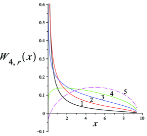
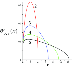
Figure 6 presents the Raney distributions $W_{p,r}(x)$ in the ”diagonal” case, $r=p$. As the distribution $W_{2,2}(x)$ represents Eq.(25), the diagonal Raney distributions, $W_{r,r}(x)$, can thus by considered as a generalization of the semicircular law: they are defined for $x\in(0,K_{r-1})$ where $K_{s}=(s+1)^{s+1}/s^{s}$, they are equal to zero at both ends of the domain and they are characterized by a single maximum. However, of $r>2$ the functions $W_{r,r}(x)$ are not symmetric anymore, compare Fig. 6. A plot of the parameter space $(p,r)$ in which these distributions are marked together with the Fuss-Catalan distributions is presented in Fig. 7.

Figure 7: Raney distributions in the parameter space $(p,r)$: Marchenko–Pastur distribution $P_{1}$ is represented by the point $(2,1)$, while Fuss-Catalan distribution $P_{s}$ is represented by $(*)$ at $(s+1,1)$. The semicircle (sc) law corresponds to $(2,2)$ and the ’diagonal’ Raney distributions $(+)$ to $(p,p)$. As shown in Ref. Ml10 any point in the shaded set $\Sigma$ corresponds to a probability measure with a compact support in $[0,\infty)$.

IV Concluding remarks

In this work we obtained an explicit form of the Fuss-Catalan distribution $P_{s}(x)$. Obtained result is exact for an arbitrary $s$ and it allows for a simple use of these probability distributions. Results derived are relevant from the point of view of statistical physics as they describe asymptotic level density of normalized positive random matrix of the product form $X=(G_{1}\cdots G_{s})(G_{1}\cdots G_{s})^{\dagger}$, where $G_{1},\dots,G_{s}$ denote $s$ independent random matrices from the complex Ginibre ensemble. The variable $x=N\lambda$ denotes the rescaled eigenvalue $\lambda$ of random matrix $X$ of size $N$.

It should be emphasized here that the Marchenko–Pastur and Fuss–Catalan distributions describe the level density of Wishart like random matrices in the limiting case $N\to\infty$ only. In practice, for any fixed $N$ the finite size effects occur. As discussed by Blaizot and Nowak BN09 ; BN10 the finite $N$ effects are related with the diffraction phenomena, while the large $N$ limit of the random matrix theory may be compared with the geometric limit of the wave optics or the semiclassical limit of the quantum theory. An explicit description of finite $N$ corrections to the spectral density of Wishart matrices obtained from products of Ginibre matrices is provided by Burda et al. BJLNS10 ; BJLNS11 .

A simple argument put forward in ZPNC10 (see Appendix B therein) implies that the same FC distributions describe also the spectral density of a product of $s$ random matrices taken from the real Ginibre ensemble LS91 . The case of a product of two real matrices, recently studied in context of quantum chromodynamics APS10 , is also important in applications in econophysics, where one uses a product of two real correlation matrices BLMM07 .

The Catalan numbers are a special case of a more general, one parameter family of Fuss-Catalan numbers, which from a subset of two-parameter family of Raney numbers. In the same way, the Marchenko–Pastur distribution $P_{1}(x)$ is a special case of the Fuss-Catalan distributions, which in turn belong to the two parameter family of Raney distributions $W_{p,r}(x)$. This wide class of probability distribution includes e.g. the Dirac delta, $\delta(x-1)$ and the semicircle law, $W_{2,2}(x)$. Applying the inverse Mellin transform for integer parameter values of the parameters we found an explicit exact representation of the Raney distributions in terms of the hypergeometric function. For any $r=1,2,\dots,p$ the Raney distribution $W_{p,r}(x)$ is supported in the interval $[0,p^{p}/(p-1)^{p-1}]$. For small $x$ the distribution behaves as

$$W_{p,r}(x)\ \sim\ \begin{cases}x^{-\frac{p-r}{p}}&\textrm{if \ $r<p$},\\ x^{\frac{1}{p}}&\textrm{if \ $r=p$}.\end{cases}$$ (33)

The Raney numbers (17) imply that the mean value of the Raney distribution $W_{p,r}(x)$ is equal to $r$, while the second moment reads $r(2p+r-1)/2$.

Let us conclude the paper with the following remark. The Fuss–Catalan distribution describe statistical properties of singular values of products of random matrices of the Ginibre ensemble. It is then natural to ask, whether there exist any ensembles of random matrices, such that their squared singular values can be described by the Raney distributions.

Acknowledgments. It is a pleasure to thank G. Akemann, Z. Burda, M. Bożejko, B. Collins, K. Górska, A. Horzela, W. Młotkowski, I. Nechita and A. M. Nowak for fruitful discussions and helpful remarks. We are thankful to both referees for useful comments. Financial support by the Transregio-12 project of the Deutsche Forschungsgemeinschaft and the grant number N N202 090239 of Polish Ministry of Science and Higher Education is gratefully acknowledged. The authors acknowledge support from Agence Nationale de la Recherche (Paris, France) under program PHYSCOMB No. ANR-08-BLAN-0243-2.

Appendix A Some information on special functions

Special functions of interest for this note are related to the Euler gamma function, which admits a following integral representation, $\Gamma(z)=\int\limits_{0}^{+\infty}t^{z-1}\,e^{-t}\,dt.$ Integrating by parts we see that $\Gamma(z+1)=z\cdot\Gamma(z)$. For an integer argument the Euler function is given by factorial, $\Gamma(n+1)=n!$ . The Gauss–Legendre formula allows one to compute the Euler gamma function of a multiple of argument MOT ,

$$\Gamma(kz)=(2\pi)^{(1-k)/2}\;k^{kz-1/2}\;\prod_{j=0}^{k-1}\Gamma\bigl{(}z+\frac{j}{k}\bigr{)}$$ (34)

for $k=1,2,3,\dots$ and $z\neq 0,-1,-2,\dots\;.$

The generalized hypergeometric series is a series in which the ratio of successive coefficients indexed by $n$ is a rational function of $n$. It can be defined as

$$\!\!{}_{p}F_{q}\bigl{(}[\{a_{j}\}_{j=1}^{p}],[\{b_{j}\}_{j=1}^{q}]\;;z):=\sum_{n=0}^{\infty}\frac{(a_{1})_{n}\dots(a_{p})_{n}}{(b_{1})_{n}\dots(b_{q})_{n}}\,\frac{z^{n}}{n!},$$ (35)

where we use the Pochhammer symbol, defined by $(a)_{n}=a(a+1)(a+2)...(a+n-1)$ and $(a)_{0}=1$.

The series (35), if convergent, defines a generalized hypergeometric function, which may then be defined over a wider domain of the argument by analytic continuation.

Note that for $s=2$ the expression (11) involves the Gauss (ordinary) hypergeometric function

$${}_{2}F_{1}([a,b],[c];\;z)=\sum_{n=0}^{\infty}\frac{(a)_{n}(b)_{n}}{(c)_{n}}\,\frac{z^{n}}{n!},$$ (36)

that includes many other special functions as special or limiting cases.

Appendix B Positivity of the distributions
$P_{s}(x)$ and $W_{p,r}(x)$

For completeness we prove in this appendix that for any integer $s$ the distribution $P_{s}(x)$ is positive for $x\in(0,K_{s})$, where $K_{s}=(s+1)^{s+1}/s^{s}$. Eq. (6) implies that $P_{s}(x)$ is given as the inverse Mellin transform of Eq. (8). We are going to use the convolution property for two Mellin transforms, ${\cal M}[f(x);\sigma]=f^{*}(\sigma)$ and ${\cal M}[g(x);\sigma]=g^{*}(\sigma)$, which reads KPS01 ; GPHDS

$${\cal M}^{-1}[f^{*}(\sigma)g^{*}(\sigma);x]=\int_{0}^{\infty}f\bigl{(}\frac{x}{t}\bigr{)}g(t)\frac{dt}{t}$$

$$=\int_{0}^{\infty}g\bigl{(}\frac{x}{t}\bigr{)}f(t)\frac{dt}{t}.$$ (37)

If $x>0$ and both functions $f(x)$ and $g(x)$ are positive then their Mellin convolution defined by the integrals (37) conserves positivity.

Consider now, for a given $j=0,1,\dots,(s-1)$, the individual term in the product in Eq.(8). Its Mellin transform will satisfy, due to formula 8.4.2.3, p.631 in PBM98 , the following equality

$${\cal M}^{-1}\Bigl{[}\frac{\Gamma\bigl{(}\sigma+\frac{j-s}{s+1}\bigr{)}}{\Gamma\bigl{(}\sigma+\frac{2+j-s}{s}\bigr{)}};\;x\Bigr{]}=\frac{x^{j-s}(1-x)^{\frac{1+s(1+j-s)}{s+1}}}{\Gamma\bigl{(}\frac{2(s+1)+js-s^{2}}{s+1}\bigr{)}}\;,$$ (38)

which for all $j=0,1,\dots,(s-1)$, is a positive function for $x\in(0,1)$. Then Eq. (8) can be viewed as a $(s-1)$–fold convolution of positive functions, which by (37) is itself positive for $x\in(0,K_{s})$. The upper edge $K_{s}$ of the support can be read off from the prefactor in Eq.(8).

In a similar way one can prove positivity of Raney distribution $W_{p,r}(x)$ for natural values of the parameters, provided $r\leq p$. Here is the streamlined version of the proof. We use the aforementioned formula 8.4.2.3 of PBM98 for $b>a$,

$${\cal M}^{-1}\Bigl{[}\frac{\Gamma(\sigma+a)}{\Gamma(\sigma+b)};x\Bigr{]}=\bigl{[}\Gamma(b-a)\bigr{]}^{-1}x^{a}(1-x)^{b-a-1},$$ (39)

which describes a positive function for $0<x<1$. We quote now the full version of the analog of Eq.(8) for $R_{p,r}(\sigma)$, with $\sigma=n+1$ and $p=2,3,\dots\;$ ,

$$R_{p,r}(\sigma) = \frac{r}{\sqrt{2\pi}}\frac{p^{r-p-1/2}}{(p-1)^{r-p+3/2}}\Bigl{[}\frac{p^{p}}{(p-1)^{p-1}}\Bigr{]}^{\sigma}\times$$ (40)

$$\times \;\frac{\Gamma\bigl{(}\sigma+\frac{r-p}{p}\bigr{)}}{\Gamma(\sigma)}\;\prod_{j=1}^{p-1}\Bigl{[}\frac{\Gamma\bigl{(}\sigma+\frac{r-p+j}{p}\bigr{)}}{\Gamma\bigl{(}\sigma+\frac{r-p+j+1}{p-1}\bigr{)}}\Bigr{]}.$$

Consider first the case $1\leq r<p$. The weight function $W_{p,r}(x)$ is the inverse Mellin transform, $W_{p,r}(x)={\cal M}^{-1}\bigl{[}R_{p,r}(\sigma);x\bigr{]}$, and, from (40) via Eq.(37), it is the $p$–fold Mellin convolution of $\Gamma[\sigma+(r-p)/p]/\Gamma(\sigma)$ and of $p-1$ factors in the product in Eq.(40). For each of these individual ratios of gamma function relation (39) holds. Therefore, with Eq.(40), the positivity of the distribution $W_{p,r}(x)$ follows.

In the second case, $r=p$, only $p-1$ factors in Eq.(40) intervene in the convolution. Hence $W_{p,p}(x)$ is also positive. If $r>p$ the first ratio in Eq.(40) destroys the positivity, so no further considerations are needed to show that in this case the function $W_{p,r}(x)$ is not a probability distribution.

Appendix C Relations between Raney distributions $W_{p,r}(x)$

The Raney distribution $W_{p,r}(x)$ may be implicitly written by its $S$-transform, which allowed Młotkowski Ml10 to establish a relation between distributions with various values of their parameters in terms of the free multiplicative convolution denoted by ${\boxtimes}$ (compare Eq. 4.10 in Ml10 ),

$$W_{1+p,1}\;{\boxtimes}\;W_{1+q,1}=W_{1+p+q,1}.$$ (41)

This result, valid for $p,q>0$, can be generalized for an arbitrary positive $r$,

$$W_{p,r}\;{\boxtimes}\;W_{1+q,1}=W_{p+rq,r}.$$ (42)

Moreover, there exists yet another relation,

$$[W_{1+p,1}]^{\boxtimes s}=W_{1+sp,1}$$ (43)

which holds for $s>0$ and is equivalent to the multiplicative convolution property for the Fuss–Catalan distribution.

References

- (1) J. Ginibre, Statistical ensembles of complex, quaternion and real matrices, J. Math. Phys. 6, 440 (1965).
- (2) M. L. Mehta, Random Matrices, 3rd ed. (Academic, New York, 2004).
- (3) J. P. Forrester, Log-gases and Random matrices (Princeton University Press, Princeton, 2010).
- (4) F. Haake, Quantum Signatures of Chaos, 3rd ed. (Springer, Berlin, 2010).
- (5) P. Šeba, Random matrix analysis of human EEG data, Phys. Rev. Lett. 91, 198104 (2003).
- (6) A. M. Tulino and S. Verdu, Random Matrix Theory and Wireless Communications (NOW Publishers Inc., 2004).
- (7) J. P. Bouchaud and M. Potters, Theory of Financial Risks: From Statistical Physics to Risk Management (Cambridge University Press, Cambridge, 2000).
- (8) Z. Burda, J. Jurkiewicz and M. A. Nowak, Is Econophysics a Solid Science?, Acta Phys. Pol. B 34, 87 (2003).
- (9) V. L. Girko, Circular laws, Theor. Prob. Appl. 29, 694 (1984).
- (10) V. A. Marchenko and L. A. Pastur, Distribution of eigenvalues for some sets of random matrices, Math. Sb. 72, 507 (1967).
- (11) A. Crisanti, G. Paladin and A. Vulpiani, Products of random matrices in Statistical Physics (Springer, Berlin, 1993).
- (12) E. Gudowska-Nowak, R. A. Janik, J. Jurkiewicz, and M. A. Nowak, Infinite products of large random matrices and matrix-valued diffusion, Nucl. Phys. B 670, 479 (2003).
- (13) J. P. Bouchaud, L. Laloux, M. A. Miceli and M. Potters, Large dimension forecasting models and random singular value spectra, Euro. Phys. J. B 55, 201 (2007).
- (14) J. C. Osborn, Universal results from an alternate random-matrix model for QCD with a baryon chemical potential, Phys. Rev. Lett. 93, 222001 (2004).
- (15) R. Lohmayer, H. Neuberger and T. Wettig, Possible large-N transitions for complex Wilson loop matrices, JHEP 11, 053 (2008).
- (16) Z. Burda, R. A. Janik and B. Wacław, Spectrum of the product of independent random Gaussian matrices, Phys. Rev. E 81, 041132 (2010).
- (17) B. Collins, I. Nechita and K. Życzkowski, Random graph states, maximal flow and Fuss-Catalan distributions, J. Phys. A 43, 275303 (2010).
- (18) K. Życzkowski, K. A. Penson, I. Nechita, and B. Collins, Generating random density matrices, preprint arXiv:1010.3570
- (19) D. Armstrong, Generalized Noncrossing Partitions and Combinatorics of Coxeter Groups, MWMO 949 (AMS Bookstore, Providence RI, 2009).
- (20) W. Młotkowski, Fuss-Catalan numbers in noncommutative probability, Documenta Math. 15, 939 (2010).
- (21) T. Banica, S. Belinschi, M. Capitaine and B. Collins, Free Bessel laws, Canadian J. Math. 63 3 (2011).
- (22) R.L. Graham, D. E. Knuth and O. Patashnik, Concrete Mathematics, (Addison–Wesley, New York 1994).
- (23) T. Koshy, Generalized Catalan Numbers, (Oxford Scholarship Online Monographs, 2008).
- (24) J. H. Przytycki and A. S. Sikora, Polygon Dissections and Euler, Fuss, Kirkman, and Cayley Numbers, J. Comb. Theory 92, 68 (2000).
- (25) N. Fuß, Solutio quaestionis, quot modus polygonum laterum in poligona laterum, per diagonales resolviquaeat, Nova acta academiæ scientiarum imperialis Petropolitanæ 9, 243 (1791).
- (26) E. Catalan, Note sur une Équation aux différences finies, J. Math. Pures Appl. 3, 508 (1838).
- (27) J. E. Koehler, Folding a Strip of Stamps, J. of Comb. Theory 5, 135 (1968).
- (28) N. Alexeev, F. Götze and A. Tikhomirov, Asymptotic distribution of singular values of powers of random matrices, Lithuanian Math. J. 50, 121 (2010) and preprint arXiv:1012.2743
- (29) M. Bożejko and W. Bryc, On a class of free Lévy laws related to a regression problem, J. Funct. Anal. 236, 59 (2006).
- (30) F. Benaych-Georges, On a surprising relation between the Marchenko-Pastur law, rectangular and square free convolutions, Ann. Inst. Poincaré Probab. Stat. 46, 644 (2010).
- (31) K. A. Penson and A. I. Solomon, Coherent states from combinatorial sequences, pp. 527-530 in Quantum theory and symmetries, Kraków 2001, (World Scientific Publ., River Edge, NJ, 2002) and preprint arXiv:quant-ph/0111151.
- (32) Z. Burda, A. Jarosz, G. Livan, M. A. Nowak and A. Świȩch, Eigenvalues and singular values of products of rectangular Gaussian random matrices, Phys. Rev. E 82, 061114 (2010).
- (33) D.-Z. Liu, C. Song, Z.-D. Wang, On explicit probability densities associated with Fuss-Catalan numbers, preprint arXiv:1008.0271.
- (34) N. J. A. Sloane, Online Encyclopedia of Integer Sequences, http://www.research.att.com/njas/sequences (2011).
- (35) N. I. Akhiezer, The Classical Moments Problem and some Related Questions in Analysis (Olivier and Boyd, Edinburgh and London, 1965).
- (36) J. R. Klauder, K. A. Penson and J.-M. Sixdeniers, Constructing coherent states through solutions of Stieltjes and Hausdorff moment problems, Phys. Rev. A 64, 013817 (2001).
- (37) K. Górska, K. A. Penson, A. Horzela, G.H.E. Duchamp and A. I. Solomon, Quasiclassical asymptotics and coherent states for bounded discrete spectra, J. Math. Phys. 51, 122102 (2010) and references therein.
- (38) K. A. Penson and K. Górska, Exact and explicit probability densities for one-sided Lévy stable distributions, Phys. Rev. Lett. 105, 210604 (2010).
- (39) P. Flajolet, X. Gourdon and P. Dumas, Mellin transforms and asymptotics: Harmonic sums, Theor. Comp. Science 144, 3-58 (1995).
- (40) A. P. Prudnikov, Yu. A. Brychkov and O. I. Marichev, Integrals and Series vol. 3: More Special Functions, (Gordon and Breach, New York, 1998).
- (41) Y. Luke, The Special Functions and their Approximations vol. 1 (Academic Press, New York, 1969).
- (42) A. Erdélyi, W. Magnus, F. Oberhettinger and F. G. Tricomi, Higher Transcendental Functions (McGraw–Hill, New York, 1953).
- (43) G. Raney, Functional composition patterns and power series reversion, Trans. Am. Math. Soc. 94, 441-451 (1960).
- (44) J. P. Blaizot and M. A. Nowak, Large Confinement, Universal Shocks and Random Matrices, Acta Phys. Pol. B40, 3321 (2009).
- (45) J. P. Blaizot and M. A. Nowak, Universal shocks in random matrix theory, Phys. Rev. E 82, 051115 (2010).
- (46) Z. Burda, A. Jarosz, G. Livan, M. A. Nowak and A. Świȩch, Eigenvalues and Singular Values of Products of Rectangular Gaussian Random Matrices (The Extended Version), preprint arXiv:1103.3964 and Acta Phys. Pol. B (2011) in press
- (47) N. Lehmann and H.-J. Sommers, Eigenvalue statistics of random real matrices, Phys. Rev. Lett. 67, 941 (1991).
- (48) G. Akemann, M. J. Phillips and H.–J. Sommers, The chiral Gaussian two-matrix ensemble of real asymmetric matrices, J. Phys. A 43, 085211 (2010).
- (49) E. P. Ozhigova, On the correspondence of Daniel Bernoulli with N. I. Fuss. Voprosy Istor. Estestvoznan. i Tekhn. 1, 108-115 (1981).